A cautionary tale: The characteristics of two-dimensional distributions and their effects on epidemiological studies employing an ecological design

Abstract

In recent years, many spatial epidemiological studies that use proximity of subjects to putative sources as a surrogate for exposure have been published and are increasingly cited as evidence of environmental problems requiring public health interventions. In these studies, the simple finding of a significant, positive association between proximity and disease incidence has been interpreted as evidence of causality. However, numerous authors have pointed out limitations to such interpretations. This, the first of two companion studies, examines the effects of analyzing (real and simulated) spatial data using logistic regression. Simulation is also employed to explore the statistical power of such analyses to detect true effects, quantify the probabilities of Type I and Type II errors, and to evaluate a proposed mechanism that explains the observed effects. Results indicate that, even when the odds ratios of cases and controls are regressed against random or nonsense sources, significant, positive associations are observed at frequencies substantially greater than chance. These frequencies increase when targets are highly non-uniformly distributed such that, for example, false-positive associations are more likely than not when odds ratios are regressed against the actual distribution of ultramafic rocks in California. The coefficients of true, causal associations are substantially attenuated under realistic conditions so that, absent corroborating analyses, there is no non-arbitrary means of distinguishing causal from spurious or real but non-causal associations. Factors affecting where people choose to live act as powerful confounders, creating spurious or real but non-causal associations between exposure and response variables (as well as between other pairs of variables). Consequently, future epidemiological studies that use proximity as a surrogate for exposure should be required to include adequate negative control analyses and/or other kinds of corroborating analyses before they are accepted for publication.

• Agent-based models
• asbestos
• causality
• clustering
• demographics
• disease-clustering
• environmental exposure
• exposure-response modeling
• geostatistics
• mesothelioma
• proximity-based exposure
• regression
• risk assessment
• spatial epidemiology

Introduction

Many spatial epidemiological studies that use proximity to putative sources as a surrogate for exposure have been recently published (e.g. Baumann et al., 2007; García-Pérez et al., 2010; Goria et al., 2009; Lopez-Abente et al., 2012; Loyo-Berrios et al., 2007; Magnani et al., 2000; Maule et al., 2007; Monge-Corella et al., 2008; Pan et al. 2005; Ramis et al., 2011). Such studies of “ecological design” are increasingly cited as evidence of environmental problems requiring public health interventions. For example, a study linking mesothelioma risk and residential proximity to outcrops of ultramafic rocks (Pan et al., 2005) has been frequently cited (e.g. Bassanese et al., 2008; Baumann et al., 2011; Case et al., 2011; Goldberg & Luce, 2005, 2009; Marchevsky et al., 2006; Plumlee et al., 2006; Roggli, 2007; Swayze et al., 2009.) to suggest increased mesothelioma risk simply from living in the general vicinity of natural occurrences of asbestos (which can be found in ultramafic rocks). This latter study is used throughout to illustrate key statistical issues and methodological caveats that are the focus of the present work.

In ecologically designed studies, significant associations between disease prevalence and proximity to putative exposure sources have been interpreted as evidence that hypothesized emissions from such sources increase risk of the adverse health effect(s) studied. However, numerous authors have pointed out the inadequacy of relying solely on such associations as evidence of causality (see Cox et al., 2013, this supplement). The validity of underlying assumptions and study designs needed for causal inferences must also be evaluated (Campbell & Stanley, 1966). When statistical regression models designed for non-spatial data (including logistic and many other types of regression commonly used in these studies) are applied to spatial data, at least two important assumptions are made: (1) that the regression models are applicable to data on a surface (e.g. that homoscedasticity and independent-errors assumptions are not invalidated by spatial correlations) and (2) that no unidentified or unaddressed sources of geographic variation between cases and controls (i.e. spatial confounders) contribute importantly to observed associations. When the former assumption is violated, the corresponding statistical tests may show significant results at frequencies greater than the nominal significance level. When the latter assumption is violated, false-positive associations may result, which would disappear in well-specified spatial statistical models (Ripley, 2004).

We evaluate these assumptions and their associated effects using geographical distributions for populations exhibiting mutually exclusive characteristics (e.g. Caucasions and Hispanics, College graduates and non-graduates), which serve as cases and controls. These are regressed against proximity to sets of physical locations used to represent putative sources. County-level and census-tract level data from the State of California (as well as simulated data) were used to define population distributions with which to test these assumptions.

This is the first of two companion studies addressing questions about epidemiological investigations with ecological designs. This study explores effects of analyzing (real and simulated) spatial data explicitly using logistic regression. Simulations are used to assess the statistical power of such analyses to detect true (causal) effects of varying magnitude, quantifying the probabilities of Type I and Type II errors. The companion study (in this same supplement) uses demographic data from California to examine effects from analyzing spatial data employing a variety of types of regression and related tools. Taken together, the findings from the two studies, encompassing both real and simulated data, appear to hold generally.

Methods

Data

Data sets used to characterize populations in this study were obtained from the California State Data Center (CSDC, 2012). Census-tract level counts of individuals were obtained directly while county-level counts were computed by summing over tracts in each county.

Age-adjusted cancer incidence rates were obtained from the California Cancer Registry (CCR, 2012) and were available by county (with some counties grouped), year (1988–2009), ethnic group (Caucasian, Black, Hispanic and Asian), and specific cancer type (Mesothelioma, Kaposi’s sarcoma [KS] and pancreatic cancer were evaluated in this study). Tract level disease incidence counts were estimated by multiplying county level incidence rates by year 2000 census-tract populations for each corresponding ethnic group divided by 100 000 (and summing over ethnic group, when needed). County level counts were found as the sum of the tract level counts within that county (which is completely equivalent to multiplying the county populations by county incidence rates).

It was also necessary to make adjustments to the cancer data from the California Cancer Registry to account for the fact that low case counts (fewer than 15) are suppressed in the public online database. Therefore data were aggregated over each 5 year interval (with 1999–2004 selected for final analysis). If values at the county level were still not available for a given county in that time interval, the state average value for that time interval and ethnic group was multiplied by the corresponding ratio of county to state values over all time periods (1988–2009). In the few cases where the latter ratio was not available, the state average value for that time interval (and ethnic group) was used for that county.

Counts of traffic accident fatalities (also used in this study) were obtained from the National Highway Transportation administration (NHTSA, 2012) and were available by year and county. County level counts were first converted to rates (fatalities per 100 000). Tract level fatality counts were then found by multiplying the county rate by the tract population counts.

Other data sets used to define the locations of targets to serve as surrogates for putative sources, including: ultramafic rocks (Krevor et al., 2009), the locations of fatal traffic accidents in 2010 (NHTSA, 2012) and the centroids of zip codes in the state (USCB, 2012) were obtained from the sources indicated. Random sets of locations were also generated for this purpose de novo using R (R Development Core Team, 2011) and the package, “Splancs” (Rowlingson & Diggle, 2012).

As indicated above, traffic fatalities are used in two independent ways in this study. County- and tract-level-counts are used to define populations at risk (serving as “cases” in some analyses) and the actual locations of fatal accidents (in 2010) are used as one of several sets of arbitrary target locations serving as putative sources.

The data specifying the locations of ultramafic rocks (Krevor et al., 2009) were contained in ArcGIS format shapefiles, with California deposits defined by 1071 irregular polygon shapes. Polygon centroids were also computed as averages of X, Y values in meters based on the Lambert Conformal Conic Projection, although distance to the nearest boundary point of each polygon was generally used to define proximity in this study. Boundaries and centroids for year 2000 census tracts and counties were obtained from the US Census Bureau (USCB, 2012). These (along with all other locations used in the study) were converted from decimal latitude and longitude to the X, Y coordinate system of the ultramafic rocks using the M_map MATLAB toolbox (Pawlowicz, 2011). Locations of ultramafic rocks in California that were evaluated in this study are shown in Figure 1 of the companion study (Cox et al., 2013).

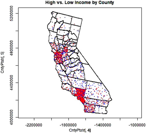
Figure 1. 1000 high-income (>2× the poverty level) earners (red) and 1000 low-income earners (blue) selected from the distributed population weighted by county-level data.

Statistical approach

A series of regressions and simulations were conducted to evaluate the probability of finding false-positive (non-causal or spurious) associations and to quantify the power to detect true-positive (causal) associations given the conditions under which these analyses are typically conducted. Additional simulations were also conducted to evaluate the underlying mechanism causing the effects observed.

About the assessment of statistical power

To assess power, it is generally necessary to know the true underlying condition of an association being analyzed (i.e. whether it is actually causal, non-causal or spurious). Thus, data are sometimes employed in this study in unconventional ways that nevertheless leave no doubt about the underlying conditions of particular analyses. Examining the anatomy of an ecological study helps to illustrate how this is accomplished.

In the kinds of ecological studies evaluated here, typically, victims of a particular disease end point are identified as cases to be studied. The set of cases is then typically matched with a set of controls that, ideally, differ from cases only in that they do not exhibit the disease. In practice, however, such matching may be imperfect. The natural logs of the odds ratios of cases versus controls are then regressed against proximity (nearest distance) to one or a set of putative sources. Given this experimental structure, tests for strictly non-causal associations are generated by:

• selecting disease end points that have no known or suspected association with the putative sources against which they are regressed. This is perhaps the weakest of the approaches used because one might be wrong in assuming no causal relation;

• selecting putative sources that do not contribute to disease, including:

  • the set of zip-code centroids;

  • the set of physical locations of fatal traffic accidents that occurred in 2010 or

  • sets of locations selected entirely at random;

• selecting individuals as cases who have no particular disease, but instead simply exhibit a particular demographic characteristic that distinguishes them from controls or

• synthesizing sets of cases and controls by a random process.

Assessing the probability of observing false-positive (non-causal) associations

Data sets containing the numbers of individuals in California counties (and, separately, census tracts) exhibiting specific characteristics were extracted from the sources referenced in the “Data” Section. Population characteristics evaluated include: the number of individuals who are Caucasian, Hispanic or Black; the number of individuals who respectively earn more or less than twice the poverty level; the number of individuals, respectively, with or without college degrees; and the number of blue collar and white collar workers. When there was a need to assure that tested associations are non-causal, subsets selected from mutually exclusive pairs of these populations were used as cases and controls (e.g. Hispanics as cases versus Caucasians as controls or college graduates versus non-college graduates). Clearly, there is no kind of exposure source that can cause one to become educated, to lose an education, to become richer or poorer, or to become Hispanic or Caucasian.

Data sets representing the age-adjusted numbers of individuals with mesothelioma, KS and pancreatic cancer (observed between 1999 and 2004) and the numbers of traffic deaths were also extracted. When regressed against random or nonsense sources, cases and controls, respectively, extracted from mutually exclusive pairs of these populations (e.g. KS cases versus pancreatic cancer controls) also assure that the associations evaluated are non-causal. Because county mesothelioma rates are not tied to occupational histories of cases in the available dataset, analyses employing this particular dataset cannot be used to examine or adjust directly for occupation, but can still be used to test for effects of proximity to specified locations.

The datasets considered in this study represent a range of population characteristics that were nevertheless both readily available and easily interpretable as numbers of individuals in specified geographical areas of California.

To evaluate the probability of obtaining false positive (non-causal) associations, stratified random sets of locations were separately generated for each set of cases and controls by randomly selecting numbers of locations in each county (or, separately, census tract) proportional to corresponding populations within that county (or census tract). Initially, more than two million locations were generated (within the State of California) for each population of interest. As a hypothetical example, suppose there are 500 000 college degreed individuals in the State and 300 in census tract #3040, then (2 000 000/500 000) * 300 random locations would be chosen for that census tract. This population-weighted sampling of locations is then repeated for each of the 7049 census tracts in the State to generate a census tract-level dataset for college degreed individuals.

Next, the set of locations in each dataset was sampled with replacement to derive 200 independent realizations of 1000 statewide locations. These represent hypothetical residences for individual cases or controls derived from their corresponding datasets. Again to illustrate, the census-tract level dataset for college degreed individuals was sampled with replacement to generate a subset of 1000 hypothetical locations representing one realization of residences for individuals with college degrees, which serve as either “cases” or “controls” in later analyses. This process was then repeated 200 times to generate 200 realizations that could be similarly analyzed so as to quantify the variability of results for such analyses.

The number of locations in each set (1000) was chosen to be comparable to the numbers of cases and controls in Pan et al. (2005). Thus, the magnitudes of odds ratios, their corresponding regression (slope) coefficients, and the power of the significance tests for regressions evaluated here and in the Pan et al. study are directly comparable. Because the total number of points in the sampled datasets (200 000 =200 × 1000) is small relative to the total number of points originally generated for each particular population (more than two million), the number of locations repeatedly sampled is also very small.

Each set of sampled distributions represents a possible realization of address-level locations for individual cases or controls that preserves the observed marginal distribution for the county- or tract-level-population from which it was derived. Thus, the frequencies of significant associations observed during regression across large numbers of such realizations indicate the probability that such an association may occur if (1) the actual addresses of all individuals were known and used to define their locations and (2) the associations are due simply to differences in the characteristics of case and control populations that are regressed against one another. These are precisely the conditions under which ecologically designed case-control studies are typically conducted. Thus, results from this study should be directly informative of any such ecologically designed study.

To complete each analysis, the natural logs of the odds ratios for cases and controls were regressed against proximity to various sets of putative sources. Sources considered include ultramafic deposits (in the same manner as Pan et al.) and two arbitrary sets: locations of 2010 traffic fatalities and zip code centroids. Each of these sets of putative sources contains approximately 2500 points (or 1100 polygons in the case of ultramafic deposits). The same pairs of cases and controls were also regressed against putative sources represented by multiple, independent sets of approximately 2500 locations that were randomly generated from within the state as a whole. With no loss of generality, only mainland California was considered (non-contiguous islands of the state were excluded).

Regressions were also conducted with cases and controls drawn from the same (single) demographic distribution. As one example, a set of random locations for cases and another for controls were independently generated from the same marginal distribution of census-tract level counts of individuals with college degrees. The dependent, dichotomous variable (indicating whether an observation is a case versus a control) was then regressed against the independent variable: distance to ultramafic deposits. This allowed us to distinguish effects attributable to confounding caused by differences between demographic populations used as cases and controls – differences which, by construction, do not exist in these (single population) runs – from effects due to other causes.

Assessing the power to detect true-positive (causal) associations

To evaluate the power to detect true (causal) associations, simulations were also conducted in which random sets of control locations were generated as described above, but case locations were generated in a manner incorporating an assumed, causal relation. This was accomplished in seven steps:

• 200 sets of 1000 locations were generated each for cases and controls in the manner previously described;

• point by point distances between each individual case and control location and each individual point in a particular set of putative sources were determined;

• the nearest distance to each case and control was identified;

• cases and controls were then stratified into categories representing successive 1 km intervals of nearest distance;

• a particular regression coefficient (for a causal association) was assumed;

• incorporating binomial variation, an adjusted number of cases (cases_adj) in each stratum of minimum distance was calculated from the number of unadjusted cases and the odds ratio for that distance derived from the assumed regression coefficient and

• the resulting cases_adj versus controls were regressed against proximity to putative sources in the same manner as previously described for evaluating false positive (non-causal) associations.

To illustrate, assuming a regression coefficient of −0.065 (corresponding to the odds ratio at standard distance of 0.937 reported by Pan et al. (2005)), the odds ratio for Case_adj/Case at 15 km would be 0.907. Noting: (1) that these values are intentionally scaled to distances in 10 km increments and (2) that the odds ratio at zero distance for Case_adj/Case can be set at 1 (so that the intercept is 0) with no loss of generality, 0.907 is derived simply as: exp[−0.065 * (15/10)]. Of course, this is the expectation value so that values actually used in the simulations would be somewhat different due to contributions from binomial variation. The number of Case_adj (N_Caseadj) at 15 km proximity in this illustration is then calculated simply as 0.907 * N_Cases. Finally, the odds ratio of Cases_adj/Controls at 15 km proximity (used in regressions to assess power) is simply set equal to N_Caseadj (at 15 km)/N_Controls (at 15 km).

Assessing the underlying mechanism

To assess the underlying mechanism driving the effects observed in this study, the complex shapes of California features were simplified, while preserving the most salient characteristics of its population (described in the following paragraphs). The most important of these characteristics (i.e. the type and extent of spatial heterogeneity between cases and controls, the centroid locations of population centers, the sizes of populations in different population centers, and the locations of putative sources) were then randomized to evaluate their overall effects. Note that both the specific shape of California and, more importantly, the specific population distribution in California were intentionally modified (with the latter also randomized) to explicitly evaluate the generality of the mechanism explored.

Simulations were carried out for populations distributed across a rectangle 1200 units long by 350 units wide (which approximate the overall dimensions of California in km). Thus, although a rectangle was used to define the outer boundaries of the state, the overall scale of California was preserved to facilitate direct comparison with other results from this study.

Initially, 50 sets of 500 “seed” locations were randomly selected within the defined rectangle to represent the centroids of hypothetical cities, towns, or rural communities. Note that this approximates the actual number of municipalities in California: 482 (League of California Cities, 2012), although their locations were randomly varied in each set of the simulations.

A relative population for each hypothetical municipality was then derived by generating 500 random variates from a lognormal distribution having a mean of 1 and standard deviation (SD) of 1.7. This provided a realistic distribution of sizes for the hypothetical municipalities (some small, most moderate, and a few very large; as in the real California). These relative populations were then multiplied by the quotient of 50 000 and the sum of the random variates to generate “absolute” populations. Thus, these simulations were scaled to an approximate ratio of 0.2% of the actual population of California, which was large enough to quantify statistical associations accurately.

To obtain the X and Y coordinates for a random set of individuals located in each hypothetical municipality, bivariate normal densities were sampled, each with a mean equal to the municipality's centroid and with an SD 10. The number of coordinates sampled from each municipality was set equal to the absolute population for that municipality, derived as described in the previous paragraph. For the scale of the map used in this simulation, an SD of 10 results in municipalities in which about 70% (±1 SD) of the population resides within 10 km of the center and approximately 92% (±2 SD's) reside within 20 km. These dimensions are reasonable for moderately sized towns. Points with coordinates lying outside of the boundaries of the rectangle representing the “stylized” California were replaced with re-sampled values. In this manner, 50 sets of 500 municipalities (with different, randomly-located centroids in each set) were surrounded in each set with newly-selected random points (proportional in number to the population of the corresponding municipality). A total of 2 513 250 stratified-random points (50 265 unique points per set) were thus generated.

To illustrate, suppose (for the first of 50 sets) Municipality #27 was assigned a centroid with XY coordinates: 100 units (east of the origin), 500 units (north of the origin) and assigned a population of 5000. The locations of residences in this municipality would be defined in two steps. First, 5000 random variates would be generated from a normal distribution with mean of 100 and an SD of 10 to represent the X coordinates of these residences. Second, 5000 random variates would be generated from a normal distribution with a mean of 500 and an SD of 10 to represent the Y coordinates of these residences. Note that if any variates generated to represent X coordinates was either negative or larger than 350 (the maximum width for the “stylized” California), it would be discarded and replaced with a re-sampled value. A similar procedure was also applied for Y coordinates.

Each of the individual locations defined as described above was then classified either as a case or a control at random, with half of the municipalities given more cases than controls and vice versa. This is how municipality-scale spatial heterogeneity was introduced. Separate datasets were generated for each of five ratios of cases to controls, to allow for sensitivity analysis of this factor: (1) 50–50% (no enrichment); (2) 60–40%, (3) 70–30%; (4) 75–25% and (5) 80–20%. These values were selected after a review of the spatial heterogeneity observed at the county and census-tract levels among the various subpopulations studied in California (see the discussion of Table 5 in “Results”).

The 50 independent sets of case and control locations were then paired with a specific set of 2500 putative source locations that were randomly generated within the same rectangle representing the stylized California. The entire process was then repeated 50 times (pairing each of the new sets of case and control locations with a new, unique set of putative source locations). This resulted in a total of 2500 unique sets (50 independent sets of case and control locations each paired with 50 independent sets of putative source locations). The process was also repeated for each of the five levels of enrichment previously defined. The final datasets were then sampled with replacement to generate 2500 sets of 1000 each of (Statewide) cases and controls, which were combined as a dichotomous variable and regressed against nearest distance (proximity) to putative sources.

The entire procedure was repeated twice. The first time, locations for putative sources were generated entirely at random within the rectangle of the “stylized” state. The second time, source locations were restricted to two north-south lines located 50 units inward from the north-south boundaries of the rectangle. This was done to represent an example of a highly non-uniform distribution of putative sources. Such a distribution loosely recalls the general pattern of ultramafic deposits within California (Cox et al., 2013: Figure 1). A more detailed discussion of the motivation for the design of these simulations is provided in “Results” as part of the discussion of mechanism.

Multiple statistical tests

Although multiple tests of significance are reported throughout these analyses, the need to reduce p values to account for multiple testing bias does not arise here. This is because, rather than drawing conclusions based on the results of individual tests, conclusions are drawn about the distributions of significance test results compared to their distribution under the null hypothesis of chance alone. Thus, for example, the frequency with which significant results are observed (compared to what would occur by chance) is one of the criteria on which conclusions are being based in these analyses.

Maps

In a few cases, locations were plotted on maps of California to illustrate the nature of the spatial distributions generated during the simulations. The base of such maps was generated by plotting the loci of points that define both the boundaries of the State of California and the individual counties within the state. The stratified random locations of cases and/or controls generated during specific simulations were then superimposed on the base map.

Software

All calculations were performed using R (R Development Core Team, 2011) and packages including: flexclust (Leisch, 2012) to determine distances between points and points or polygons, reshape (Wickam, 2011) to assist with data preparation, and splancs (Rowlingson & Diggle, 2012) to generate random points within defined areas. Maps were also generated using R (R Development Core Team, 2011).

Results

Figure 1 is a map of the state of California with the county boundaries indicated. Superimposed on this map is a distribution of 2000 points, half (the red points) representing households with incomes greater than twice the poverty level and half (the blue points) representing individuals with lower income. As can be seen in the figure, points are relatively concentrated in some counties while others are sparse. Also, some counties are redder and others bluer. Such a pattern should not be surprising as the distribution is driven primarily by total population (which varies substantially between counties) and secondarily by differences in where individuals in differing socioeconomic categories choose (or can afford) to live.

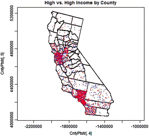
Figure 2 is similar to Figure 1, except that the red points and the blue points represent two different realizations (two independently selected sets of random points weighted by county population) of the same high income earners depicted in Figure 1. Thus, differences between the distributions of red and blue points in Figure 2 are due to chance alone. As can be seen by comparing the sparser counties in Figures 1 and 2, the total number of points in each county of Figure 2 is approximately double the number of red points observed in the same county in Figure 1. This is because both cases and controls in Figure 2 are derived from the same distribution represented in Figure 1 by the red points alone; the low income earners (blue points in Figure 1) were ignored in Figure 2. Consequently, as expected, points in each county are more evenly divided between red and blue in Figure 2 than in Figure 1. The same general patterns to those described for Figures 1 and 2 are consistent with figures derived using data representing each of the other population characteristics evaluated as cases and controls in this study. However, the details are subtly different for different pairs of population characteristics (not shown).

Figure 2. Two independent sets of 1000 high-income earners; one representing cases (red) and the other representing controls (blue) selected from the distributed population weighted by county-level data.

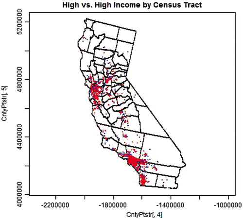
Figures 3 and 4 repeat Figures 1 and 2, respectively, except that populations are weighted by census tracts instead of counties. Consequently, populations tend to be more highly concentrated in more limited areas, but the results are otherwise similar. This should not be surprising as (1) the population distribution in California is highly non-uniform and (2) Figures 3 and 4 are closer to the true distribution because the resolution at which the distributions are constrained by actual information is substantially higher in these figures than Figures 1 and 2; there are 7049 census-tracts but only 58 counties in California.

Figure 3. 1000 high-income (> 2× the poverty level) earners (red) and 1000 low-income earners (blue) selected from the distributed population weighted by census-tract-level data.

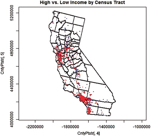
Figure 4. Two independent sets of 1000 high-income earners; one representing cases (red) and the other representing controls (blue) selected from the distributed population weighted by census-tract-level data.

It should be clear from such figures that the number of individuals exhibiting particular ethnic, educational or socio-economic traits varies from county to county and census tract to census tract and that the nature of such variation is a unique feature of the particular characteristic being evaluated, which in turn reflects where such individuals choose to live.

Assessing the probability of observing a false-positive (non-causal) association

To evaluate the probability of observing false positive (non-causal) associations using logistic regression, odds ratios from pairs of cases and controls (representing populations with mutually exclusive characteristics) were each regressed against distances from sets of actual physical locations serving as putative sources in California. Because they were used as surrogates for sources of asbestos in Pan et al. (2005), the locations of ultramafic rocks are of particular interest and were therefore evaluated first.

Table 1 summarizes results from 200 independent datasets each containing 1000 locations representing cases and 1000 locations representing controls. The natural log of the odds ratio for being a case instead of a control was regressed against proximity to ultramafic rocks for the variables listed in the table, which include a range of demographic and risk characteristics. As previously indicated, the unconventional use of two populations distinguished by a specific demographic characteristic (to serve respectively as cases and controls) assures that no causal association with proximity to sources can exist for these analyses (see Statistical Approach in “Methods”).

Table 1. Results of logistic regression comparing ORs for cases versus controls to proximity to ultramafic deposits in California*.

	Including data from all California counties				Excluding data from six southern California counties†
Indicated “cases” versus “controls”	OR‡	UCL¶	LCL§	P_OR||	OR‡	UCL¶	LCL§	P_OR||
Tract-level data
College degree versus no college degree	0.9648	0.9837	0.9492	1.7E−04	0.9081	0.9357	0.8786	1.5E−11
Income more than 2× poverty level versus less	0.9722	0.9921	0.9523	2.9E−03	0.9466	0.9651	0.9170	3.0E−06
White collar versus blue collar	0.9835	1.0037	0.9654	7.5E−02	0.9854	1.0075	0.9544	2.3E−01
Caucasian versus Hispanic	0.9579	0.9732	0.9387	6.2E−06	0.9466	0.9651	0.9170	3.0E−06
Caucasian versus black	0.9919	1.0070	0.9716	3.7E−01	0.9736	0.9931	0.9462	1.6E−02
Black versus Hispanic	0.9639	0.9799	0.9469	1.8E−04	0.9827	1.0062	0.9624	9.2E−02
Caucasian versus Caucasian#	1.0004	1.0162	0.9777	5.2E−01	1.0015	1.0245	0.978	5.1E−01
KS** versus pancreatic cancers**	1.0090	1.0292	0.9878	2.8E−01	0.9156	0.9415	0.8815	1.6E−10
Mesotheliomas** versus pancreatic cancers**	1.0054	1.0215	0.9884	4.4E−01	0.9984	1.018	0.9756	4.8E−01
Traffic fatalities versus pancreatic cancers**	1.0168	1.0353	0.9993	5.9E−02	1.0600	1.0887	1.0357	4.0E−07
County-level data
College degree versus no college degree	0.9752	0.9864	0.9633	1.0E−04	0.9579	0.9719	0.9388	2.4E−08
Income more than 2× poverty level versus less	0.9835	0.9969	0.9709	7.1E−03	0.9792	0.9910	0.9642	8.5E−04
White collar versus blue collar	0.9914	1.0032	0.9793	1.8E−01	1.0012	1.0145	0.9860	4.8E−01
Caucasian versus Hispanic	0.9751	0.9857	0.9619	4.1E−05	0.9691	0.9823	0.9568	3.8E−07
Caucasian versus Caucasian#	1.0001	1.0140	0.9897	5.3E−01	1.0005	1.0119	0.9868	5.2E−01
KS†† versus pancreatic cancers††	1.0031	1.0156	0.9906	4.6E−01	0.9664	0.9800	0.9485	2.2E−06
Mesotheliomas†† versus pancreatic cancers††	1.0045	1.0166	0.9913	3.3E−01	1.0006	1.0107	0.9909	4.7E−01
Traffic fatalities versus pancreatic cancers††	1.0153	1.0275	1.0032	6.6E−03	1.0247	1.0388	1.0129	4.4E−05

*The natural logs of the odds ratios for cases versus controls were regressed against proximity to ultramafic rocks. In each regression, street-address level locations for cases and controls were separately chosen at random within each county (or census tract) with numbers proportional to their respective population within that county (or census tract). A total of 1000 each of cases and controls were selected statewide during each iteration. Results represent the 50th percentiles of 200 independent regressions. UCLs and LCLs respectively represent the 97.5th and 2.5th percentiles of the resulting OR's.

†The six southern California counties eliminated are: Imperial, Los Angeles, Orange, Riverside, San Diego and Ventura. These were eliminated because they contain virtually no ultramafic deposits.

‡This is the OR at standard distance for the indicated association. It is the exponential of the regression coefficient and can be interpreted to represent the fractional decrease (or increase, if greater than one) in “risk” with every 10 km increase in distance. Regressions were scaled to 10 km distances in this study so that the magnitude of the coefficients would be directly comparable to those reported by Pan et al. (2005). Boxed values show larger effects than those reported by Pan et al.

¶This is the two-tailed 95% upper confidence limit on the OR.

§This is the two-tailed 95% lower confidence limit on the OR.

||This is the p value for the OR (and the corresponding regression coefficient). By convention, values of 0.05 or less are considered significant and are therefore bolded and italicized.

#Caucasians versus Caucasians represent regressions in which the locations of cases and controls were derived from the same marginal distribution (Caucasians) so that any “non-uniform” heterogeneity (defined in the accompanying text) between cases and controls is eliminated. Thus, these runs serve as negative controls because no effect is expected.

**Cases and controls for cancers are based on sampling the distribution of estimated cancers derived as the product of the (annualized) age-adjusted rate per 100 000 in the indicated county multiplied by the at-risk population in the corresponding county (divided by 100 000). County data were then extrapolated to tract-level data by obtaining counts for individual ethnic groups as the product of the county-rate and the tract-level population of each ethnicity and summing over ethnic groups.

††Numbers of countywide cases and controls were derived as described in the previous footnote.

Results on the top of Table 1 represent distributions derived based on tract-level data with results on the bottom derived based on county-level data. Results presented on the left represent regressions using data from all of California and those on the right are from regressions excluding data from the six southernmost California counties: Imperial, Los Angeles, Orange, Riverside, San Diego and Ventura. These counties were excluded because they contain virtually no ultramafic deposits (e.g. Cox et al., 2013: Figure 1; Pan et al., 2005).

As can be seen by the p values in Columns 5 and 9 (Labeled: “P_OR”) of Table 1, many distinguishing characteristics within the population of California (i.e. most of the ones tested) exhibit significant associations with distance to ultramafic rocks. Considering the data from all of California, eight of the 16 tested associations (50%) are significant. Moreover, at a 0.1% level of significance, the associations between distance to ultramafic rock and both white- versus blue-collar workers and traffic fatalities versus pancreatic cancers are also significant (making 63% of the analyses positive).

A similar pattern holds with the six southern California counties excluded, although the levels of significance are generally greater (p values are smaller). A larger number of significant associations (69% and 75% at the 0.05 and 0.1 levels of significance, respectively) is also observed. This is expected because, as previously indicated, the lack of ultramafic deposits in Southern California would cause case and control points in these counties to contribute most to the largest absolute distances from ultramafics while (at such distances) the relatively smaller distances between cases and controls would have a corresponding, attenuated effect on their relative proximity. At the same time, because approximately half of the population of California resides in these six counties, they would contribute half of the points to most distributions. Table 1 also indicates that results are generally similar whether county-level or tract-level data are employed to define cases and controls.

Importantly, the two tests of Caucasians versus Caucasians (shaded in Table 1) are not included in the denominators of the frequencies described in the previous paragraphs, as these two runs serve as negative control analyses. These analyses compare cases and controls representing separate realizations from the same marginal distribution (proportion of Caucasians) and, therefore, should not be significant. In fact, they both show p values of approximately 0.5 (50%), which is exactly what would be expected for the median value of a properly functioning significance test. Moreover, these analyses exhibit an approximately 5% rate of significant results (p values < 0.05) among the 200 independent runs conducted (data not shown). Again, this is exactly as expected, given a 5% target level of significance for these tests, meaning that the null hypothesis may be falsely rejected by chance alone in up to 5% of cases where it is true. Similar negative-control analyses were also conducted for most of the other characteristics listed in the table (e.g. college degreed individuals versus college degreed individuals) with all results showing the same pattern as the Caucasian versus Caucasian analyses (data not shown).

As previously suggested in the discussions of Figures 1–4, the primary difference between distributions of cases and controls derived from the same population and those derived from different populations is the type of spatial heterogeneity. Distributions of cases and controls derived from the same population (e.g. Caucasians) exhibit only spatially “random” heterogeneity (cases and controls occupy independent sets of random locations within each geographical unit, but their numbers in each unit are identical). Those derived from different populations exhibit “non-uniform” heterogeneity resulting from differences in the numbers of cases and controls in each county or census tract (depending on which type of data was used to define them). Thus, results in Table 1 suggest that real but non-causal associations (false positives) tend to result from non-uniform heterogeneity. Moreover, the scale of the heterogeneity does not appear to matter; false positives result whether non-uniform heterogeneity occurs at the scale of counties or census tracts. In contrast, effects disappear in those analyses involving only spatially random heterogeneity.

Results obtained by regressing the natural log of the odds ratios of the same pairs of cases and controls against the locations of fatal traffic accidents in 2010 and the centroids of zip codes (both serving as “nonsense” sources) show generally similar patterns to those displayed in Table 1. However, the number of data sets showing significant associations is somewhat lower (data not shown). Nevertheless, the number of data sets with non-uniform heterogeneity that show significant results (when regressed against all of the sets of physical locations tested) is substantially greater than the 5% that would otherwise be expected by chance alone.

The interpretation of results from Table 1 (and the additional analyses involving nonsense sources) warrants scrutiny. As previously indicated, living closer to ultramafic rocks (or zip code centroids or the locations of traffic accidents) does not cause an individual to be Caucasian versus Hispanic or Black, white collar versus blue collar, have a college degree versus not or have a higher income. There is also no published evidence that exposure to asbestos (or any other component of ultramafic rocks) causes KS so that the significant finding that KS victims live closer to ultramafics (and zip code centroids, results not shown) than pancreatic cancer victims has no clear causal interpretation either. Thus, these statistically significant associations are almost certainly false positives in terms of causality. Yet, the frequency and strength of the significant associations reported in Table 1 show that such associations are the rule, rather than the exception. This raises serious questions about the validity of concluding causality simply from finding a significant association when applying logistic regression to these types of data.

Tables 2 and 3 present results from regressing the same characteristics in Table 1 against multiple realizations of randomly selected source locations. Table 2 presents results from county-level data and Table 3 presents analogous results for tract-level data. Both are based on 200 regressions against independent sets of 2500 source locations (50 sets for county-level analyses and 27 sets for tract-level analyses). Because the locations of putative sources are random, any significant associations observed in these analyses must be non-causal (and may be spurious).

Table 2. Estimates of ORs, intercepts and frequencies for cases versus controls regressed against sets of random sources (county-level data)*.

Cases	Controls	OR†	LTail‡ OR	UTail¶ OR	Fraction significant (%)§	Fraction steeper (%)||	Fraction increasing (%)#	Fraction decreasing (%)**	Intercept	LTail‡ intercept	UTail¶ intercept	Fraction significant (%)††
County-level data from all counties in California
Caucasians	Hispanics	0.9898	0.7279	1.3539	10	68	47	53	1.0065	0.8259	1.2301	7
Caucasians‡‡	Caucasians‡‡	1.0025	0.7754	1.2914	5	62	51	49	0.9984	0.8496	1.1758	3
Caucasians	Blacks	1.1464	0.5499	2.5840	56	89	62	38	0.9179	0.5675	1.5046	51
Blacks	Hispanics	0.8612	0.3824	1.8714	56	89	36	64	1.0983	0.6554	1.7891	51
White collar workers	Blue collar workers	1.0066	0.7708	1.3071	5	63	52	48	0.9958	0.8433	1.1799	3
College graduates	Non-college graduates	1.0161	0.7657	1.3417	7	65	54	46	0.9899	0.8281	1.1836	4
Income > twice poverty level	Income ≤ twice poverty level	1.0098	0.7636	1.3252	7	65	53	47	0.9938	0.8361	1.1881	4
Mesotheliomas	Pancreatic cancers	1.0109	0.7750	1.3168	5	62	54	46	0.9932	0.8421	1.1745	3
KS	Pancreatic cancers	0.9603	0.6600	1.4725	21	77	42	58	1.0260	0.7730	1.2852	16
Traffic deaths	Pancreatic cancers	0.9946	0.7493	1.3515	8	66	48	52	1.0034	0.8301	1.2062	5
County-level data excluding six counties in southern California¶¶
Caucasians	Hispanics	1.0106	0.7517	1.3348	7	66	53	47	0.9933	0.8324	1.1937	4
Caucasians‡‡	Caucasians‡‡	1.0003	0.7683	1.3042	5	63	50	50	0.9998	0.8459	1.1823	3
Caucasians	Blacks	1.2455	0.3217	5.8225	72	93	62	38	0.8720	0.3848	2.2568	68
Blacks	Hispanics	0.8160	0.1659	3.1830	70	93	38	62	1.1356	0.4367	2.6386	67
White collar workers	Blue collar workers	1.0098	0.7697	1.3245	6	64	53	47	0.9940	0.8362	1.1766	3
College graduates	Non-college graduates	1.0195	0.7287	1.4067	12	70	55	45	0.9879	0.8014	1.2156	8
Income > twice poverty level	Income ≤ twice poverty level	1.0179	0.7539	1.3554	8	67	55	45	0.9888	0.8234	1.1908	5
Mesotheliomas	Pancreatic cancers	1.0127	0.7689	1.3354	6	65	54	46	0.9920	0.8344	1.1810	3
KS	Pancreatic cancers	0.8784	0.5022	2.0835	59	91	39	61	1.0843	0.6059	1.5078	54
Traffic deaths	Pancreatic cancers	0.9945	0.7380	1.3491	9	68	49	51	1.0036	0.8293	1.2148	5

*The natural logs of the ORs for cases versus controls were regressed against proximity to sets of (2500) random locations. In each regression, street-address level locations for cases and controls were separately chosen at random within each county with numbers proportional to their respective population within that county. A total of 1000 each of cases and controls were selected state-wide during each iteration. OR results represent the 50th percentile of 10 000 regressions grouped as 200 sets of cases and controls regressed against each of 50 independent sets of (2500) random locations.

†This is the OR at standard distance for the association. It is the exponential of the regression coefficient and can be interpreted to represent the fractional decrease (or increase if greater than one) in “risk” with every 10 km increase in distance. Regressions were scaled to 10 km distances in this study so that the magnitude of the coefficients would be directly comparable to those reported by Pan et al. (2005).

‡This is the lower tail (2.5th percentile) of the distribution of OR's observed across all (50 × 200 = 10 000) regressions.

¶This is the upper tail (97.5th percentile) of the distribution of OR's observed across all (50 × 200 = 10 000) regressions.

§This is the fraction of regressions (200 × 50 = 10 000) for which the OR (and, correspondingly, the regression coefficient) was observed to be significant.

||This is the fraction of regressions for which a greater absolute OR (i.e. < 0.937 or >1.067) is observed than that reported by Pan et al. 2005. Note that 1.067 is the reciprocal of 0.937, which simply represents an increasing (rather than decreasing) trend.

#This is the fraction of regressions for which an OR greater than 1 is observed, which is equivalent to a positive regression coefficient and means that the number of cases increases with distance from putative sources.

**This is the fraction of regressions for which an OR less than 1 is observed, which is equivalent to a negative regression coefficient and means that the number of cases decreases with distance from putative sources.

††This is the fraction of regressions for which the intercept was observed to be significant.

‡‡Caucasians versus Caucasians represent regressions in which the locations of cases and controls were derived from the same marginal distribution (Caucasians), so that any “non-uniform” heterogeneity (defined in the text accompanying Table 1) between cases and controls is eliminated. Thus, these runs which are highlighted, serve as negative controls because no effect is expected.

¶¶Counties excluded from these analyses are: Imperial, Los Angeles, Orange, Riverside, San Diego and Ventura.

Table 3. Estimates of ORs, intercepts and frequencies for cases versus controls regressed against distance to random sources (tract-level data)*.

Cases	Controls	OR†	LTail‡ OR	UTail¶ OR	Fraction significant (%)§	Fraction steeper (%)||	Fraction increasing (%)#	Fraction decreasing (%)**	Intercept	LTail‡ intercept	UTail¶ intercept	Fraction significant (%)††
Tract-level data from all counties in California
Caucasians	Hispanics	0.9527	0.4773	1.6084	33	79	42	58	1.0311	0.7506	1.6364	26
Caucasians‡‡	Caucasians‡‡	1.0040	0.7749	1.3065	5	61	52	48	0.9975	0.8456	1.1740	3
Caucasians	Blacks	0.9517	0.3456	2.2278	62	89	46	54	1.0325	0.6275	2.0954	58
Blacks	Hispanics	1.0913	0.3816	2.7705	58	92	57	43	0.9470	0.4813	1.7699	52
White collar workers	Blue collar workers	0.9810	0.7152	1.3476	11	68	45	55	1.0120	0.8295	1.2346	7
College graduates	Non-college graduates	0.9737	0.6611	1.4354	19	74	45	55	1.0171	0.7926	1.2945	14
Income > twice poverty level	Income ≤ twice poverty level	0.9793	0.6345	1.4587	21	74	46	54	1.0131	0.7885	1.3492	15
Mesotheliomas¶¶	Pancreatic cancers¶¶	1.0012	0.7571	1.3163	6	64	50	50	0.9993	0.8428	1.1866	3
KS¶¶	Pancreatic cancers¶¶	0.9549	0.5963	1.6738	32	81	43	57	1.0292	0.7089	1.3583	26
Traffic fatailities¶¶	Pancreatic cancers¶¶	1.0091	0.7235	1.4144	12	70	52	48	0.9945	0.8100	1.2285	8
Tract-level data excluding six counties in southern Californial
Caucasians	Hispanics	0.9108	0.5657	1.4699	28	79	33	67	1.0601	0.7872	1.4563	23
Caucasians‡‡	Caucasians‡‡	0.9967	0.7586	1.3087	5	64	49	51	1.0021	0.8428	1.1859	3
Caucasians	Blacks	0.9567	0.3895	2.5858	54	87	45	55	1.0283	0.5811	1.9604	51
Blacks	Hispanics	0.9808	0.3523	2.5632	47	85	48	52	1.0121	0.5057	1.8618	43
White collar workers	Blue collar workers	1.0075	0.6886	1.3978	13	71	51	49	0.9953	0.8090	1.2517	8
College graduates	Non-college graduates	0.9705	0.5764	1.4403	21	75	44	56	1.0187	0.7862	1.3788	17
Income > twice poverty level	Income ≤ twice poverty level	1.0110	0.6567	1.6264	29	82	51	49	0.9932	0.7345	1.3039	23
Mesotheliomas¶¶	Pancreatic cancers¶¶	1.0021	0.7442	1.3400	7	66	51	49	0.9987	0.8346	1.2012	4
KS¶¶	Pancreatic cancers¶¶	0.7896	0.4068	2.9863	68	92	31	69	1.1519	0.4549	1.6705	64
Traffic Fatailities¶¶	Pancreatic cancers¶¶	1.0217	0.6679	1.4476	14	73	55	45	0.9870	0.7953	1.2883	10

*The natural logs of the ORs for cases versus controls were regressed against proximity to sets of (2500) random locations. In each regression, street-address level locations for cases and controls were separately chosen at random within each census tract with numbers proportional to their respective population within that census tract. A total of 1000 each of cases and controls were selected statewide during each iteration. OR results represent the 50th percentile of 5400 regressions grouped as 200 sets of cases and controls regressed against each of 27 independent sets of (2500) random locations (unless otherwise indicated; see Footnote ¶¶).

†This is the OR at standard distance for the association. It is the exponential of the regression coefficient and can be interpreted to represent the fractional decrease (or increase if greater than one) in “risk” with every 10 km increase in distance. Regressions were scaled to 10 km distances in this study so that the magnitude of the coefficients would be directly comparable to those reported by Pan et al. (2005).

‡This is the lower tail (2.5th percentile) of the distribution of OR's observed across all regressions.

¶This is the upper tail (97.5th percentile) of the distribution of OR's observed across all regressions (either 5400 or 10 000 depending on the population; see Footnote ¶¶).

§This is the fraction of regressions (200 × 27 = 5400 or 200 × 50 = 10 000 for indicated populations, see Footnote ¶¶) for which the OR was observed to be significant.

||This is the fraction of regressions for which a greater absolute OR (i.e. < 0.937 or >1.067) is observed than that reported by Pan et al. (2005). Note that 1.067 is the reciprocal of 0.937, which simply represents an increasing (rather than decreasing) trend.

#This is the fraction of regressions for which an OR greater than 1 is observed, meaning that the number of cases increases with distance from target locations (putative sources).

**This is the fraction of regressions for which an OR less than 1 is observed, meaning that the number of cases decreases with distance from target locations (putative sources).

††This is the fraction of regressions for which the intercept was observed to be significant.

‡‡Caucasians versus Caucasians represent regressions in which the locations of cases and controls were derived from the same marginal distribution (Caucasians) so that any “non-uniform” heterogeneity (defined in the text accompanying Table 1) between cases and controls is eliminated. Thus, these runs which are highlighted, serve as negative controls because no effect is expected.

¶¶Regressed against each of 50 independent sets of 2500 random locations chosen within the State of California.

§§Counties excluded from these analyses are: Imperial, Los Angeles, Orange, Riverside, San Diego and Ventura.

As can be seen in Column 6 of Table 2, the following variables show significant odds ratios (and their corresponding regression coefficients) more than 50% of the time (i.e. more often than not): Caucasians versus Blacks and Blacks versus Hispanics (both with all counties included or with southern counties excluded); and KS versus pancreatic cancers (with southern counties excluded). Several additional variables show significant associations more than 10% of the time (double the 5% expected by chance). In contrast, as expected, regressions between cases and controls derived from the same underlying data (Caucasians versus Caucasians, shaded rows in the table) yield significant associations close to the 5% expected by chance.

Tract-level data generally produce even greater frequencies of significant associations (Column 6 of Table 3). In fact, with the exception of the shaded rows representing negative control analyses (which yield 5% frequencies, as expected) and the singular pair of mesothelioma cases versus pancreatic cancer controls, every other pair of cases and controls yields frequencies of significant associations greater than 10% (twice what is expected by chance) and most exceed 20%.

Comparing results between Table 1 (Columns 2 and 6) and Tables 2 and 3 (Column 3), it can be seen that all significant regressions in Table 1 (except those involving traffic fatalities) involve odds ratios that are less than one (meaning that the number of cases decreases relative to controls with increasing distance from source locations). Correspondingly, all upper confidence limits (UCL's) of the corresponding odds ratios for significant associations (except those involving traffic fatalities) are less than one. However, this is simply an artifact of the manner in which cases (versus controls) between regressed pairs were intentionally defined; reverse the definitions and all smaller odds ratios would become greater than one (and equal to the reciprocals of the odds ratios shown). Similarly, the odds ratio for traffic fatalities would become less than one.

In contrast, Tables 2 and 3 show that all lower tails (LTail's – Column 4) for the distribution of odds ratios are less than one and all upper tails (UTail's – Column 5) are greater than one. When cases and controls are regressed against specific, fixed sources (such as ultramafic rocks in Table 1), any observed associations would be expected either to be increasing (greater than one) or decreasing (less than one) with distance, but not both. This is because the differences between cases and controls will have a definite direction relative to a fixed set of source locations. Such associations are considered real but (for these regressions) non-causal.

However, when multiple sets of sources are selected at random (as for results presented in Tables 2 and 3), some sets of source locations should result in an increasing odds ratio between cases and controls (because the selected sources are closer to controls) and others should show a decreasing association (because sources are closer to cases). This is precisely what is observed in Tables 2 and 3.

LTail's and UTail's in Tables 2 and 3 represent percentiles of the distribution of odds ratios observed across regressions involving multiple sets of sources. They therefore indicate the range of odds ratios observed across these tests, but are not directly related to the significance of any particular test. Thus, the fraction of regressions observed to be significant in these tests is presented in Column 6 of Tables 2 and 3. In contrast, the LCL's and UCL's (in Table 1) represent percentiles of the distribution of odds ratios from repeated regressions involving multiple realizations of cases and controls regressed against a single, specific set of sources (the locations of ultramafic rocks). Thus, they legitimately represent confidence limits for the odds ratios observed.

Columns 8 and 9 show the relative frequencies of increasing versus decreasing odds ratios observed for each pair of cases and controls presented in Tables 2 and 3. That some increase and some decrease for every pair of cases and controls (every row in the table) suggest these associations are non-causal and spurious (over the universe of possible sets of sources). For any single set of sources, however, they either increase or decrease and thus should be considered “real” but non-causal.

The frequencies of significant results among sets of regressions listed in Tables 2 and 3 (Column 6) are generally and substantially (although not exclusively) less than those for corresponding sets of regressions listed in Table 1 (not shown). Possible explanations for this difference are addressed in the “Mechanism” and “Discussion” Sections and in Cox et al. (2013).

Comparing results here to those reported by Pan et al., the column headed “Fraction Steeper” in Tables 2 and 3 indicate that the odds ratios observed during these regressions are generally steeper (further from one). This means the corresponding associations are generally stronger. However, as expected, because multiple sets of source locations are being compared, odds ratios in Tables 2 and 3 (Column 3) are sometimes decreasing (less than one) and sometimes increasing (greater than one); if increasing, odds ratios are considered steeper if they are larger than the reciprocal of those reported by Pan et al. The two framed odds ratios in Table 1 are also steeper than those reported by Pan and coworkers. Thus, the magnitude of the odds ratio reported by Pan et al. should be considered unremarkable relative to those caused by false positives (whether spurious or real but non-causal).

The relationship between odds ratios and intercepts indicated in Tables 2 and 3 is constrained by the fact that equal numbers of cases and controls were employed in all regressions, so odds ratios and intercepts are negatively correlated. As seen in Tables 2 and 3, when odds ratios are smaller than one (meaning that the ratio of cases and controls decreases with increasing distance), intercepts are greater than one (meaning that the number of cases at zero distance is larger than the number of controls) and vice versa. The levels of significance for odds ratios and intercepts are also correlated.

Assessing the power to detect true-positive (causal) associations

Table 4 presents results of simulations conducted with odds ratios for causal associations assumed (see the discussion of true positives in the “Methods” Section or Footnotes * and † of the table for details). As indicated in the first column of the table, three assumed odds ratios were selected for evaluation (in addition to a value of 1 – signifying no causal effect). As can be seen by the corresponding regression (slope) coefficients (reported in the 2nd column), selected values are equal to, four times, and sixteen times the slope corresponding to the Pan et al. (2005) reported odds ratio of 0.937.

Table 4. Results from simulating the distribution of population characteristics within census tracts to evaluate associations with proximity to ultramafic rock*.

Assumed slopes/OR's†		Cases have college degree controls don't‡					Cases have > 2 × poverty level Income controls don't‡					Cases are white collar controls are blue collar¶
OR	Slope§	Observed OR||	Observed slope§	OR UCL95#	OR LCL95**	p Value††	Observed OR||	Observed slope§	OR UCL95#	OR LCL95**	p Value††	Observed OR||	Observed slope§	OR UCL95#	OR LCL95**	p Value††
Casesadj versus Controls
1	0	0.916	−0.088	0.941	0.890	1.9E−11	0.950	−0.051	0.971	0.928	7.1E−07	0.982	−0.018	1.001	0.964	9.2E−02
0.937	−0.065	0.911	−0.094	0.935	0.877	1.3E−16	0.941	−0.061	0.963	0.919	5.6E−11	0.976	−0.025	0.996	0.953	1.5E−02
0.771	−0.260	0.891	−0.116	0.913	0.860	3.1E−20	0.921	−0.082	0.941	0.896	9.1E−16	0.958	−0.043	0.979	0.933	1.0E−04
0.353	−1.041	0.794	−0.231	0.830	0.748	1.6E−31	0.832	−0.184	0.866	0.799	3.8E−30	0.880	−0.128	0.905	0.843	3.9E−15
Controls versus Casesadj
1	0	1.091	0.087	1.130	1.067	1.6E−11	1.054	0.053	1.078	1.030	3.2E−07	1.018	0.018	1.038	0.999	9.2E−02
0.937	−0.065	1.087	0.084	1.121	1.057	2.5E−11	1.047	0.046	1.074	1.022	4.0E−06	0.948	−0.054	0.976	0.919	3.0E−06
0.771	−0.260	1.069	0.067	1.103	1.040	2.3E−07	1.028	0.027	1.056	1.007	7.1E−03	0.931	−0.072	0.962	0.906	5.8E−09
0.353	−1.041	0.999	−0.002	1.027	0.969	4.6E−01	0.963	−0.037	0.988	0.940	2.2E−03	0.880	−0.128	0.905	0.843	3.9E−15
Casesadj versus Cases
1	0	1.000	0.000	1.029	0.976	5.3E−01	1.001	0.001	1.021	0.976	4.8E−01	1.001	0.001	1.020	0.977	4.8E−01
0.937	−0.065	0.993	−0.007	1.020	0.963	3.9E−01	0.992	−0.008	1.015	0.972	3.1E−01	0.994	−0.006	1.005	0.977	6.1E−01
0.771	−0.260	0.975	−0.026	0.994	0.952	6.4E−03	0.972	−0.028	0.996	0.951	7.8E−03	0.976	−0.025	0.987	0.963	5.9E−02
0.353	−1.041	0.903	−0.103	0.934	0.865	5.0E−09	0.901	−0.105	0.933	0.875	7.0E−13	0.904	−0.101	0.921	0.885	1.2E−09

*Results of logistic regression of Cases_adj versus Controls, Controls versus Cases_adj or Cases_adj versus Cases with closest distance to ultramafic deposits as the independent variable. In each regression, street-address level locations for controls were separately chosen at random within each census tract with numbers proportional to their population within that census tract. Case_adj locations were similarly chosen at random, but with numbers proportional to a population within each census tract estimated (with binomial variation) as the product of the assumed OR and the number of unadjusted cases in that census tract. A total of 1000 each of cases and controls were selected statewide during each iteration. For all of the analyses presented, populations in Imperial, Los Angeles, Orange, Riverside, San Diego and Ventura Counties were excluded from the calculations.

†These are the (assumed) OR at standard distance and the corresponding slopes used to calculate the populations of adjusted cases whose relative distances to ultramafics were compared to the indicated, second population using logistic regression. As detailed in the Methods section (and Footnote * above), estimated populations were also calculated by incorporating binomial variation about their expectation value.

‡Results based on 200 iterations.

¶Results based on 100 iterations.

§These highlighted columns show the regression (slope) coefficients corresponding to the odds ratios presented in the previous columns. In logistic regression, the exponential of the slope coefficients represent the odds ratios at standard distance between cases and controls. Nevertheless, typically, it is the OR's themselves that are reported in studies employing logistic regression.

||These are the observed OR's for the association between the indicated characteristic and the distance to ultramafic rock. Values less than one indicate that the population of cases decreases relative to controls as distance from ultramafic rock increases. Values greater than one indicate that cases increase relative to controls at increasing distance.

#These upper confidence bounds represent the 97.5th percentile of the observed distribution of observed OR's over the indicated number of iterations.

**These lower confidence bounds represent the 2.5th percentile of the observed distribution of observed OR's over the indicated number of iterations.

††These p values indicate the significance of the test of whether the observed OR's differs from one (and, correspondingly, whether the regression coefficient differs from zero). Significant values are bolded.

To facilitate the remaining discussion of Table 4, comparisons will be addressed using regression (slope) coefficients (presented in the shaded columns of the table), where the lack of an effect conveniently shows no slope (a value of zero), while true (assumed) slopes (Column 2) or observed slopes (Columns 4, 9 and 14) can either be positive (increasing) or negative (decreasing). An increasing slope means that cases become more numerous relative to controls as distance increases and vice versa. Results in Table 4 show that observed slopes are always attenuated relative to underlying true slopes, as expected in the presence of (nondifferential) measurement error of a single independent variable (Armstrong, 1990). In multi-variate regression, however, measurement error may introduce bias either toward or away from the null (Rosner et al., 1990).

Table 4 is divided into three sections, respectively, showing results when the innate slopes between cases and controls reinforce, counter or are neutral to assumed (causal) relationships. Innate slopes are the slopes attributable to non-uniform heterogeneity between cases and controls, which are observed when the causal effect (represented by the assumed slope) is set to zero in the simulation that generates the data values. The upper third of the table (labeled “Cases_adj versus Controls”) presents cases versus controls having negative innate slopes, which reinforce the assumed slopes (all negative) that were used to generate case_adj locations. In the middle third (labeled “Controls versus Cases_adj”), cases and controls are reversed so that they all have positive innate slopes, which counter the assumed (causal) slopes. The bottom third (“Cases_adj versus Cases”) shows cases versus themselves, which have no non-uniform heterogeneity so that the innate slope is zero.

As is apparent in all three sections of Table 4, observed slopes decrease monotonically as increasingly negative assumed slopes (representing causal associations) are introduced. In all cases, however, the magnitude of changes in observed slopes are small relative to those of the corresponding assumed slopes. This confirms that causal associations are attenuated whether the innate slopes reinforce, counter, or are neutral to the assumed slopes. Moreover, due to the attenuation, observed slopes are more similar to (driven primarily by) their corresponding innate slopes (representing non-causal effects from non-uniform heterogeneity) than to corresponding assumed slopes (representing underlying causal associations).

Specifically when innate slopes run counter to assumed slopes (middle of Table 4), the magnitudes of the observed slopes first decrease toward zero (from a positive innate slope) before changing sign and becoming increasingly negative as the underlying causal association (represented by the assumed slopes) increases in magnitude (becomes more negative). Thus, there will always be a value for an underlying assumed slope at which the observed slope becomes zero and all evidence of any association (causal or not) completely disappears. For cases lacking college degrees versus controls having degrees, for example the observed slope becomes zero when the underlying, assumed slope is −1.041, which is 16 times steeper than the slope corresponding to the odds ratio (0.937) reported by Pan et al. This effect can go in either direction so that true (causal) associations with positive slopes can also be masked when countered by a negative innate (non causal) association. Thus, there is no non-arbitrary way to determine whether an observed slope represents a true (causal) association or not.

Assessing the underlying mechanism(s)

As reported above, the probability of finding a significant association by regressing a dichotomous variable (cases versus controls) against proximity to a set of sources is no different from what one would expect by chance, as long as the locations of cases and controls are drawn from a common distribution (e.g. California Caucasians) so that there is no non-uniform heterogeneity in locations. However, the probability is substantially greater than expected by chance (although the associations are non causal) when the locations of cases and controls are drawn from two different populations (e.g. Caucasians versus Hispanics or Blacks, individuals with incomes more than twice the poverty level versus those with less, individuals with college degrees versus those without), which are non-uniformly heterogeneous. Thus, it appears that false positives are driven primarily by non-uniform heterogeneity rather than random heterogeneity.

Such observations should not be surprising if one considers that people tend to choose where they live at least partly intentionally, rather than at random. They live in places they can afford. They live close to work or close to transportation to work. Depending on how they define themselves, they may also choose to live in communities with similar ethnic, cultural or religious traits or, perhaps, in close proximity to other family members. This is why, for example many large cities have “Chinatowns” or “little Italy's”. Such differences (which may not even be entirely identifiable) can cause the residential distribution of any two selected groups of individuals to differ (i.e. can create non-uniform heterogeneity). We hypothesize that such differences can suffice to cause one group or another to appear to live significantly closer to any arbitrary set of sources. If true, such associations would have nothing to do with any putative interaction between source locations and the groups being compared; they would clearly be non-causal.

Why the above-stated hypothesis is likely true is evident from the following thought experiment. Consider two municipalities founded at some distance from one another (with locations chosen either at random or intentionally). Assume that, due to some important population characteristic related to personal identity, one municipality tends to attract one kind of individual and the other a different kind. Consider further that, at the extreme, the attraction might be so compelling that each municipality attracts individuals of their own kind to the complete exclusion of others. The result would be two distinct municipalities that are individually homogeneous. Because the centroids of these two municipalities are different, clearly (with limited exceptions) the distance between each municipality and any single (arbitrarily defined) source would also have to be different. Moreover, once each municipality grew beyond a population of only about seven members, logistic regression would show that the difference in distance to the source would be significant (calculation not shown). The only exception to the above would occur if the chosen source fell precisely on a line bisecting and perpendicular to the line linking the centroids of the two municipalities.

Next, consider the case of multiple sources, if the entire area over which these distributions exist have no boundaries, than a uniform distribution of sources might also result in sets of distances from those in the case municipality and those in the control municipality that are similar. On any finite surface with boundaries that are closer in some places to one municipality than the other (which would be true for any realistic situation), however, even a uniformly distributed set of sources will necessarily be closer on average to one municipality than the other. Importantly, whether considering proximity to either one or multiple sources, it is not the locations of the particular municipalities that matter; it is the differences in the relative numbers of each group that settle in each municipality (i.e. the degree of non-uniform heterogeneity) that matters.

Clearly, for any real situation, the separation of any two large and heterogeneous populations that nevertheless exhibit a differing mix of characteristics is unlikely to be so extreme as to result in them residing in mutually exclusive municipalities. However, those with similar characteristics are nevertheless more likely to live closer to one another than those with less similar characteristics. Based on the results of our findings already reported, such clustering appears to be sufficient to substantially increase the probability of finding one of the two groups to be significantly closer to any arbitrary set of putative sources.

It is interesting that differences in demographic distributions might plausibly come about by a random action (the initial settlement of the first set of individuals of two different groups across an area) followed by directed enhancement (or filtering): once an initially random set of communities build or acquire features that attract other individuals of like characteristics, individuals with characteristics matching one group or the other might preferentially settle closer to those of similar kind. This then creates sufficient offsets in the centroids of the two groups that one or the other will tend to be closer to any set of putative sources (given that all locations are on a finite surface with boundaries that limit the range of possible sources). These conjectures are consistent with the rich literature on agent-based models of action, which (among other things) have been used to describe how communities develop and segregate (e.g. Clark & Fossett, 2008; Fagiolo et al. 2007; Fossett & Dietrich, 2009; Jordan et al., 2011) as pioneered by Schelling (1969, 1978). The plausibility of the novel hypothesis that such differences (once established) can drive the outcome of epidemiological studies of ecological design is addressed below.

Simulations were conducted to assess the reasonableness of the hypothesis that the observed differences in proximity are due to individuals tending to live closer to others sharing similar characteristics, even though such characteristics are independent of any specific association with the source locations against which proximity is being evaluated. To conduct such simulations, individuals were assumed to reside in municipalities that are somewhat enriched (relative to chance) in those sharing similar characteristics (relative to those not sharing such characteristics) and factors such as the population sizes, locations and degree of enrichment of such municipalities were varied to assure that results of the simulations can be generalized. Details of the manner in which the simulations were implemented are provided in the discussion on mechanism in the “Methods” Section as well as in the footnotes of the data tables discussed below.

Before conducting these simulations, reasonable values for the degree of enrichment in simulated municipalities were derived from California demographic data. Table 5 presents an analysis of the relative enrichment of “cases” or “controls” in each census tract and county of California for each of the population characteristics previously discussed.

Table 5. Observed ratios of “Cases” versus “Controls” for indicated characteristics among the 7049 census tracts and 58 counties in California*.

Ratios: cases to controls		Fraction of observed ratios at least as extreme as indicated ratios
Relative	Absolute	Reciprocal	Higher versus lower income (%)†	College degree versus none (%)	White collar versus blue collar (%)	Caucasians versus Hispanics (%)	Caucasians versus blacks (%)	Mesothelioma versus pancreatic (%)	KS versus pancreatic (%)	Traffic deaths versus pancreatic (%)
Census tract data
	0.1	10.00	3	6	7	21	27	0	0	0
	0.2	5.00	15	19	17	40	45	0	3	0
	0.3	3.33	31	33	28	55	58	0	13	0
	0.4	2.50	44	47	38	66	67	0	20	2
	0.5	2.00	57	59	49	74	74	0	25	10
	0.6	1.67	67	69	60	81	81	1	38	32
	0.7	1.43	76	78	70	87	86	4	72	78
	0.8	1.25	85	86	81	92	91	23	84	85
80/20	0.25	4	23	26	22	49	52	0	7	0
75/25	0.33	3	35	37	31	59	61	0	14	1
70/30	0.43	2.33	48	50	41	68	69	0	20	2
60/40	0.67	1.5	73	75	67	85	85	2	43	47
50/50	1.00	1	99	100	100	100	100	100	100	100
County data
	0.1	10.00	0	0	0	9	33	3	5	0
	0.2	5.00	0	0	0	28	47	3	12	3
	0.3	3.33	0	0	3	40	59	3	26	9
	0.4	2.50	3	24	7	50	66	7	38	29
	0.5	2.00	12	33	16	57	74	7	43	47
	0.6	1.67	29	59	24	66	76	14	50	66
	0.7	1.43	53	67	38	81	81	22	55	78
	0.8	1.25	67	72	64	90	88	47	62	90
80/20	0.25	4	0	0	0	34	55	3	17	3
75/25	0.33	3	0	7	5	43	62	3	29	12
70/30	0.43	2.33	5	24	10	50	66	7	38	29
60/40	0.67	1.5	47	59	33	76	79	16	52	72
50/50	1.00	1	100	100	100	100	100	100	100	100

*Each cell of this table represents the fraction of counties (or census tracts) in which the ratio of cases to controls (or controls to cases) is more extreme than the indicated ratio. Thus, for example, “24%” in the fifth column of the shaded row near the bottom of the table representing a ratio of 70/30 (70% to 30%) in the column for College degrees versus none (cases being those with a college degree and controls having no degree) indicates that 24% of California Counties show ratios of cases versus controls (or controls versus cases) of 70/30 or more extreme for these populations. Highlighted rows represent ratios equal to or bracketing a ratio of 70/30. Percentages of geographic units exceeding indicated “case/control” ratios that are greater than 50% are bolded

†This is the number of individuals with an income that is twice the poverty level versus less.

Each cell of Table 5 represents the fraction of counties (or census tracts) in which the ratio of cases to controls (or controls to cases) is more extreme than the ratio indicated in the same row (described in different ways in each of the first three columns). Thus, for example “24%” in the fifth column of the shaded row near the bottom of the table, representing a ratio of 70/30 (70% to 30%) in the column for College degrees versus none indicates that 24% of California Counties show ratios of cases versus controls (or controls versus cases) of at least 70/30 for this population pair. Note that the data in this table have nothing directly to do with regressions, odds ratios or p values; they only indicate the extent of non-uniform heterogeneity observed across counties and census tracts.

As can be seen at the bottom of the table, more than a quarter of California counties show enrichment for most of the population pairs listed that is more extreme than 70% to 30% and most counties show enrichment that is more extreme than 60% to 40%. Similarly, as seen in the middle of the table, more than 40% of census tracts show enrichment that is more extreme (for most of the indicated population pairs) than 70% to 30% and almost half of the census tracts show enrichment more extreme than 60% to 40% (for nearly all of the listed population pairs). Also, almost a third of census tracts show enrichment more extreme than 75% to 25% for a majority of the pairs listed. Comparing results for specific pairs of populations in Tables 1 and 5, it is apparent that population pairs showing a significant association with proximity to ultramafic rocks also show among the most extreme enrichment over the highest fraction of counties or census tracts. Therefore, ranges of enrichment similar to (or bounding) those described here were considered during these simulations (see “Methods” section).

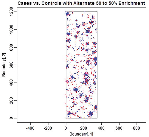
Figures 5 and 6 each show one realization of the simulated distributions of 1000 cases (in red) and 1000 controls (in blue) living among “enriched” municipalities. Both Figures 5 and 6 depict distributions sampled from a set of 500 clusters (simulated municipalities) with the same range of sizes and centered in the same locations. The figures differ, however, in the selection of the random subset of points (representing individual residences) sampled from each municipality. Also, Figure 5 depicts a distribution with 70% to 30% enrichment and Figure 6 depicts a distribution with 50% to 50% (no enrichment).

Figure 5. 1000 Cases (red) and 1000 Controls (blue) sampled from a set of 500 simulated “municipalities” of randomly varying sizes and locations with a randomly selected half weighted to favor cases (70%/30%) and the other half favoring controls (70%/30%).

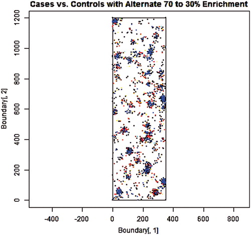
Figure 6. 1000 Cases (red) and 1000 Controls (blue) sampled from a set of 500 simulated “municipalities” of randomly varying sizes and locations with each weighted equally (50%/50%), neither favoring cases or controls.

As can be seen in the figures, cases and controls are indeed concentrated into clusters (simulated municipalities) that are dispersed randomly throughout the stylized State, although the precise locations of smaller municipalities are not as obvious as the larger ones. In fact, it is somewhat difficult to identify which points come from which unique municipality, due to a combination of overlap and the fact that smaller municipalities may be represented in the limited sample by as few as one (or even zero) points. There are also substantial (white) areas with no apparent population. Also, due to the substantial enrichment, several of the municipalities in Figure 5 are substantially redder or bluer than others. In contrast, municipalities in Figure 6 (where there is no enrichment) are more evenly mixed in color.

Comparing Figures 5 and 6 with Figures 3 and 4, it is evident that the features described in the previous paragraph are common to both sets of figures. Thus, the simulations conducted to evaluate our hypothesis concerning the mechanism producing false positive associations appears to have adequately captured the general features of interest (i.e. they capture effects causing and driven by non-uniform heterogeneity). At the same time, the two sets of figures clearly differ in the overall uniformity of their respective distributions; Figures 5 and 6 show a much more uniform distribution of municipalities than Figures 3 and 4. This illustrates two points. First, the simulations conducted to generate Figures 5 and 6 address a more general range of possibilities than the actual population distribution in California; given sufficient iterations, more highly skewed distributions such as those depicted in Figures 3 and 4 will occasionally, although rarely, occur. Therefore, conclusions drawn from these simulations should reasonably apply both to California and to any other location generally. Second, as depicted in Figures 3 and 4, the actual population distribution in California is highly non-uniform. As already addressed, however, it is not the overall population distribution that is important, only the non-uniform heterogeneity superimposed on that distribution that affects creation of false positives.

Table 6 presents summary statistics across all of the 2500 regressions conducted for each degree of enrichment evaluated. Column 2 of Table 6 shows that, when there is no enrichment (the 50% to 50% row), regressions that result in significant associations occur at the 5% rate consistent with chance alone. However, when cases tend to live nearer to cases and controls nearer to controls, the fraction of significant associations increases with increasing enrichment. This is entirely consistent with the observations previously reported indicating that non-uniform heterogeneity causes false positive (non-causal) associations to occur at frequencies greater than expected by chance alone. Also, as expected,

• the median odds ratio observed for each data set (Column 2) remains close to one because cases and controls were regressed against multiple, random sets of putative sources (so that some would be expected to be closer to cases and others to controls). In fact, as can be seen in Columns 7 and 8, about half of the odds ratios are greater than one and half less. Thus, it is not surprising that the median OR value from each dataset remains close to one;

• the median intercepts observed for each data set show the same pattern as odds ratios, because they are correlated and

• a substantial fraction (≥63%) of slopes are steeper than the slope (0.937) reported by Pan et al. (2005), even though they all clearly represent non-causal associations (i.e. randomly selected locations regressed against randomly selected sources).

Table 6. Summary results of four sets of 2500 regressions conducted to test a hypothetical mechanism underlying the excessive numbers of false-positive (non-causal) associations observed among California demographic data*.

Degree of Enrichment†	OR‡	LTail¶ OR	UTail§ OR	Fraction significant (%)||	Fraction steeper (%)#	Fraction increasing (%)**	Fraction decreasing (%)††	Intercept	LTail¶ intercept	UTail§ intercept	Fraction significant (%)‡‡
50–50%	1.0011	0.7773	1.2884	5	63	50	50	0.9992	0.8472	1.1801	3
70–30%	0.9935	0.7260	1.3865	13	71	48	52	1.0043	0.8066	1.2360	9
75–25%	1.0044	0.6937	1.4440	17	72	51	49	0.9971	0.7836	1.2732	13
80–20%	0.9985	0.6711	1.5048	22	74	50	50	1.0010	0.7668	1.2972	17

*Based on 50 realizations of 1000 cases and 1000 controls regressed against each of 50 independent sets of 2500 random locations chosen within a rectangle representing a “stylized” California. Cases and controls were each located by a stratified random mechanism described in the “mechanism discussion” of the “Methods” section of the text. A total of 2500 regressions (50 realizations × 50 sets) were completed overall.

†This is the relative fraction of cases versus controls in each of 500 simulated municipalities of varying sizes randomly located across a stylized State of California.

‡This is the median of 2500 estimates of the OR at standard distance (which is the exponential of the regression coefficient) for the association. It can be interpreted to represent the fractional decrease (or increase if greater than one) in “risk” with every 10 km increase in distance. Regressions were scaled to 10 km distances in this study so that the magnitude of the coefficients would be directly comparable to those reported by Pan et al. (2005).

¶This is the lower tail (2.5th percentile) of the distribution of OR's (or intercepts) observed across all 2500 regressions.

§This is the upper tail (97.5th percentile) of the distribution of OR's (or intercepts) observed across all 2500 regressions.

||This is the fraction of the 2500 regressions for which the OR (and correspondingly the regression coefficient) was observed to be significant.

#This is the fraction of regressions for which a greater absolute OR (i.e. < 0.937 or >1.067) is observed than that reported by Pan et al. (2005). Note that 1.067 is the reciprocal of 0.937, which simply represents an increasing (rather than decreasing) trend.

**This is the fraction of regressions for which an OR greater than 1 is observed, which is equivalent to a positive regression coefficient and means that the number of cases increases with distance from putative sources.

††This is the fraction of regressions for which an OR less than 1 is observed, which is equivalent to a negative regression coefficient and means that the number of cases decreases with distance from putative sources.

‡‡This is the fraction of the 2500 regressions for which the intercept was observed to be significant.

Table 7 presents the distribution (percentiles) of the same 50 sets of 50 regressions with the median values highlighted. Note that the median values in Table 7 are close, but not identical, to the summary values for datasets representing corresponding degrees of enrichment in Table 6. This is due to Table 7 presenting percentiles of summaries over subsets while Table 6 presents summaries over the combined subsets. Also, because values for the percentiles of each factor (e.g. odds ratio or fraction increasing) presented in Table 7 are derived from the distribution for that factor in isolation, values for different factors in the same row are not directly relatable (unlike Table 6). That is why, for example the “Fraction Increasing” and the “Fraction Decreasing” in any row do not necessarily sum to one in Table 7.

Table 7. Distribution of results from sets of regressions conducted to test a hypothetical mechanism underlying the excessive numbers of false-positive associations observed among California demographic data*.

Percentiles†	OR‡	Ltail¶ OR	Utail§ OR	Fraction significant (%)||	Fraction steeper (%)#	Fraction increasing (%)**	Fraction decreasing (%)††	intercept	Ltail¶ intercept	UTail§ intercept	Fraction significant (%)††
Percentiles of 50 iterations of 50 regressions each (assumed: 50–50% – no enrichment among cases and controls)
Min	0.9556	0.6405	1.2031	0	50	36	40	0.9764	0.7826	1.1185	0
5th%ile	0.9767	0.6976	1.2261	0	54	42	43	0.9830	0.7978	1.1300	0
10th%ile	0.9814	0.7194	1.2321	2	54	44	44	0.9855	0.8082	1.1376	0
20th%ile	0.9876	0.7289	1.2519	2	58	46	46	0.9910	0.8236	1.1445	0
50th%ile	1.0032	0.7736	1.2908	4	62	52	48	0.9979	0.8477	1.1801	2
80th%ile	1.0142	0.8107	1.3491	6	68	54	54	1.0084	0.8639	1.2261	4
90th%ile	1.0225	0.8203	1.3716	8	72	56	56	1.0120	0.8720	1.2428	6
95th%ile	1.0268	0.8289	1.4134	9	72	57	58	1.0152	0.8735	1.2646	6
Max	1.0366	0.8419	1.4599	12	78	60	64	1.0303	0.8876	1.3340	8
Percentiles of 50 iterations of 50 regressions each (assumed: 70–30% enrichment of cases or controls among 500 municipalities)
Min	0.9010	0.6171	1.2524	2	54	32	32	0.9496	0.7275	1.1511	2
5th%ile	0.9345	0.6416	1.3022	6	60	34	37	0.9695	0.7522	1.1745	2
10th%ile	0.9436	0.6539	1.3127	8	60	40	40	0.9768	0.7648	1.1905	4
20th%ile	0.9591	0.6870	1.3376	10	62	40	46	0.9855	0.7790	1.2116	6
50th%ile	0.9985	0.7177	1.4067	14	72	50	50	1.0010	0.7998	1.2412	8
80th%ile	1.0226	0.7468	1.4619	18	76	54	60	1.0272	0.8279	1.2742	12
90th%ile	1.0348	0.7667	1.4986	18	80	60	60	1.0376	0.8374	1.3162	14
95th%ile	1.0475	0.7806	1.5429	20	82	63	66	1.0446	0.8434	1.3393	17
Max	1.0846	0.8072	1.6218	24	92	68	68	1.0728	0.8651	1.3829	22
Percentiles of 50 iterations of 50 regressions each (assumed: 75–25% enrichment)
Min	0.9455	0.5836	1.3153	4	54	28	30	0.9552	0.6926	1.1253	2
5th%ile	0.9510	0.6095	1.3329	10	64	40	37	0.9681	0.7126	1.1737	7
10th%ile	0.9590	0.6332	1.3621	12	66	42	40	0.9702	0.7332	1.2230	8
20th%ile	0.9811	0.6528	1.3846	14	66	44	42	0.9819	0.7499	1.2342	8
50th%ile	1.0037	0.6852	1.4559	17	72	51	49	0.9975	0.7800	1.2822	12
80th%ile	1.0280	0.7218	1.5438	20	78	58	56	1.0124	0.8090	1.3339	16
90th%ile	1.0471	0.7383	1.6075	24	80	60	58	1.0278	0.8183	1.3533	18
95th%ile	1.0504	0.7851	1.6681	26	80	63	60	1.0332	0.8295	1.3849	20
Max	1.0705	0.8317	1.7424	28	82	70	72	1.0363	0.8354	1.4293	26
Percentiles of 50 iterations of 50 regressions each (assumed: 80–20% enrichment)
Min	0.9449	0.5331	1.3637	10	58	38	36	0.9301	0.6922	1.1945	8
5th%ile	0.9518	0.5815	1.3798	13	66	40	38	0.9658	0.7057	1.2231	10
10th%ile	0.9612	0.6124	1.4092	16	68	42	40	0.9736	0.7111	1.2364	12
20th%ile	0.9658	0.6233	1.4535	16	68	44	44	0.9832	0.7328	1.2644	12
50th%ile	0.9966	0.6660	1.5114	22	74	50	50	1.0023	0.7620	1.3090	16
80th%ile	1.0260	0.7011	1.6064	26	80	56	56	1.0225	0.7830	1.3641	20
90th%ile	1.0427	0.7182	1.6721	30	80	60	58	1.0259	0.7992	1.3797	22
95th%ile	1.0555	0.7382	1.6944	32	82	62	60	1.0333	0.8117	1.4059	23
Max	1.1186	0.7632	1.7728	40	86	64	62	1.0378	0.8169	1.4923	40

*Based on 50 realizations of 1000 cases and 1000 controls regressed against each of 50 independent sets of 2500 random locations chosen within a rectangle representing a “stylized” California. Cases and controls were each located by a stratified random mechanism described in the “mechanism discussion” of the Methods Section of the text. A total of 2500 regressions (50 realizations × 50 sets) were completed overall.

†These are the percentiles of the distributions of the indicated factors observed across 50 sets of regressions. Median values are highlighted. Each of the 50 sets contains 50 independent realizations of 1000 randomly generated cases and controls with the natural log of their odds ratios regressed against nearest distance to a particular set of 2500 putative sources. A different (randomly selected) set of sources was generated for each of the 50 sets of regressions.

‡This is the OR at standard distance (which is the exponential of the regression coefficient) for the association. It can be interpreted to represent the fractional decrease (or increase if greater than one) in “risk” with every 10 km increase in distance. Regressions were scaled to 10 km distances in this study so that the magnitude of the coefficients would be directly comparable to those reported by Pan et al. (2005).

¶This is the lower tail (2.5th percentile) of the distribution of OR's (or intercepts) observed across the 50 regressions (each incorporating a unique realization of locations for cases and controls) within a single set. The percentiles reported for the tails in the table are observed across the 50 sets (each set incorporating a distinct set of hypothetical sources).

§This is the upper tail (97.5th percentile) of the distribution of OR's (or intercepts) observed across the 50 regressions (each incorporating a unique realization of locations for cases and controls) within a single set. The percentiles reported for the tails in the table are observed across the 50 sets (each set incorporating a distinct set of hypothetical sources).

||This is the fraction of the 2500 regressions for which the OR (and correspondingly the regression coefficient) was observed to be significant.

#This is the fraction of regressions for which a greater absolute OR (i.e. < 0.937 or >1.067) is observed than that reported by Pan et al. (2005). Note that 1.067 is the reciprocal of 0.937, which simply represents an increasing (rather than decreasing) trend.

**This is the fraction of regressions for which an OR greater than 1 is observed, which is equivalent to a positive regression coefficient and means that the number of cases increases with distance from putative sources.

††This is the fraction of regressions for which an OR less than 1 is observed, which is equivalent to a negative regression coefficient and means that the number of cases decreases with distance from putative sources.

‡‡This is the fraction of the 50 regressions from each set for which the intercept was observed to be significant.

Of most interest in Table 7 is a percentile-to-percentile comparison across the blocks representing different degrees of enrichment (different degrees of non-uniform heterogeneity). That the fractions significant (Column 4) are uniformly larger (for every corresponding percentile) in the three datasets in which communities are enriched than in the dataset representing no enrichment indicates that each of these data sets produce false-positive associations at rates significantly greater than expected by chance alone. Moreover, (again for every corresponding percentile) there is a uniformly increasing trend in fractions significant with increasing enrichment (increasing non-uniform heterogeneity). Best estimates (the medians) suggest that they produce false positive associations at rates approaching 15% (for enrichment of 70–30%), exceeding 15% (for enrichment of 75–25%) and exceeding 20% (for enrichment of 80–20%). Thus, it appears that our hypothesis can reasonably explain why comparisons of groups of individuals exhibiting differing population characteristics tend to show false-positive (non-causal) associations with proximity to any intentionally or arbitrarily selected set of putative sources.

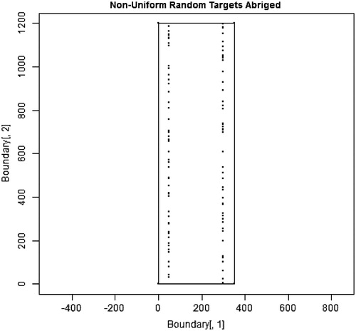
To test whether more highly skewed (non-uniform) location distributions of cases, controls and/or sources increases the chance of finding a significant, false-positive (non-causal) association, we repeated the simulations described above, but restricted the 2500 source locations to lie along two vertical lines that are each 50 km inward from the north–south boundaries of the rectangle representing the stylized State of California. In these latter simulations, 1250 points were scattered randomly along each vertical line.

Figures 7 and 8, respectively, present one set of 2500 randomly located source points from the first set of simulations and one set of restricted, random locations from the second set of simulations. The difference in the uniformity of the two distributions is immediately obvious.

Figure 7. 2500 source locations uniformly distributed around the stylized state.

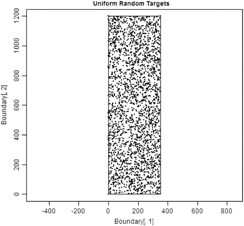
Figure 8. 100 source locations distributed non-uniformly along two vertical lines that are each 50 km inward from the north-south boundaries of the stylized state. Note that the number of locations was reduced from 2500, so that the random nature of the distribution along each vertical line could be easily observed.

Table 8 presents results from this second set of simulations. Like Table 7, it shows the percentiles of the results across the 50 sets of 50 regressions each. Without enrichment, the probability of finding a false-positive (non-causal) association remains at the expected 5% in Table 8 and a percentile-to-percentile comparison across tables shows that results for these two corresponding blocks of data are closely comparable. With enrichment, the probability of finding a false-positive association is substantially greater when putative sources are non-uniformly distributed (Table 8) then when sources are uniformly distributed (Table 7), at least for the types of non-uniform distributions evaluated. Both Tables 1 and 8 indicate that, under fairly common circumstances, when sources are non-uniformly distributed, the probability of observing a false-positive (non-causal) association is more likely than not.

Table 8. Distribution of results from sets of regressions conducted to test a hypothetical mechanism underlying the excessive numbers of false-positive associations observed among California demographic data and highly non-uniform target locations*.

Percentiles†	OR‡	Ltail¶ OR	Utail§ OR	Fraction significant (%)||	Fraction steeper (%)#	Fraction increasing (%)**	Fraction decreasing (%)††	Intercept	Ltail¶ intercept	UTail§ intercept	Fraction significant (%)‡‡
Percentiles of 50 iterations of 50 regressions each (assumed: 50–50% – no enrichment)
Min	0.9950	0.9651	1.0164	0	0	36	36	0.9816	0.8343	1.0738	0
5th%ile	0.9965	0.9684	1.0188	0	0	40	41	0.9843	0.8456	1.0944	0
10th%ile	0.9969	0.9706	1.0197	2	0	42	42	0.9890	0.8535	1.1070	0
50th%ile	1.0002	0.9756	1.0242	4	0	50	50	0.9991	0.8821	1.1386	0
90th%ile	1.0021	0.9808	1.0308	8	0	58	58	1.0149	0.9032	1.1733	4
95th%ile	1.0031	0.9829	1.0318	9	0	59	60	1.0192	0.9079	1.1858	4
Max	1.0038	0.9860	1.0361	16	0	64	64	1.0249	0.9137	1.2262	6
Percentiles of 50 iterations of 50 regressions each (assumed: 60–40% enrichment)
Min	0.9928	0.9492	1.0209	6	0	34	34	0.9667	0.7620	1.1465	2
5th%ile	0.9940	0.9518	1.0251	10	0	36	37	0.9730	0.7777	1.1527	4
10th%ile	0.9953	0.9536	1.0265	10	0	40	40	0.9810	0.7814	1.1620	4
50th%ile	0.9990	0.9649	1.0373	18	0	48	52	1.0049	0.8298	1.2056	10
90th%ile	1.0038	0.9709	1.0472	24	0	60	60	1.0257	0.8682	1.3043	16
95th%ile	1.0049	0.9712	1.0515	27	0	63	64	1.0311	0.8781	1.3171	17
Max	1.0063	0.9736	1.0534	32	0	66	66	1.0356	0.8927	1.3606	20
Percentiles of 50 iterations of 50 regressions each (assumed: 70–30% enrichment)
Min	0.9896	0.9260	1.0359	26	0	32	32	0.9453	0.6565	1.1975	18
5th%ile	0.9927	0.9280	1.0427	30	0	38	38	0.9503	0.6770	1.2650	22
10th%ile	0.9933	0.9307	1.0471	34	0	40	42	0.9690	0.6851	1.2766	24
50th%ile	1.0006	0.9434	1.0592	42	2	50	50	0.9971	0.7350	1.3604	30
90th%ile	1.0066	0.9551	1.0760	52	6	58	60	1.0337	0.7857	1.4438	40
95th%ile	1.0098	0.9564	1.0802	52	6	62	62	1.0368	0.8039	1.4969	41
Max	1.0107	0.9622	1.0858	60	12	68	68	1.0580	0.8163	1.5129	44
Percentiles of 50 iterations of 50 regressions each (assumed: 75–25% enrichment)
Min	0.9900	0.9204	1.0677	42	2	38	46	0.9773	0.5901	1.3625	36
5th%ile	0.9917	0.9223	1.0724	44	4	40	48	0.9824	0.6087	1.3833	38
10th%ile	0.9928	0.9243	1.0746	46	6	40	48	0.9904	0.6157	1.3899	38
50th%ile	0.9969	0.9326	1.0855	50	9	46	54	1.0159	0.6500	1.4527	43
90th%ile	1.0017	0.9390	1.0963	56	12	52	60	1.0376	0.6891	1.5376	48
95th%ile	1.0035	0.9421	1.0975	59	13	52	60	1.0464	0.6964	1.5474	50
Max	1.0044	0.9464	1.1074	62	14	54	62	1.0540	0.7089	1.5619	52
Percentiles of 50 iterations of 50 regressions each (assumed: 80–20% enrichment)
Min	0.9808	0.8965	1.0509	40	4	30	34	0.9008	0.4739	1.2193	34
5th%ile	0.9889	0.9015	1.0552	44	6	40	38	0.9193	0.5645	1.3974	37
10th%ile	0.9912	0.9037	1.0617	46	6	42	40	0.9285	0.5857	1.4134	42
50th%ile	1.0002	0.9236	1.0869	58	12	50	50	0.9991	0.6425	1.5284	49
90th%ile	1.0142	0.9370	1.1089	64	20	60	58	1.0482	0.7296	1.7100	56
95th%ile	1.0161	0.9399	1.1178	67	22	62	60	1.0575	0.7563	1.7809	59
Max	1.0217	0.9573	1.1518	78	24	66	70	1.1130	0.7708	1.8832	60

*Based on 50 realizations of 1000 cases and 1000 controls regressed against each of 50 independent sets of 2500 random locations chosen within a rectangle representing a “stylized” California. Cases and controls were each located by a stratified random mechanism described in the “mechanism discussion” of the “Methods” section of the text. A total of 2500 regressions (50 realizations × 50 sets) were completed overall.

†These are the percentiles of the distributions of the indicated factors observed across 50 sets of regressions. Median values are highlighted. Each of the 50 sets contains 50 independent realizations of 1000 randomly generated cases and controls with the natural log of their OR regressed against nearest distance to a particular set of 2500 putative sources. A different (randomly selected) set of sources was generated for each of the 50 sets of regressions.

‡This is the OR at standard distance (which is the exponential of the regression coefficient) for the association. It can be interpreted to represent the fractional decrease (or increase if greater than one) in “risk” with every 10 km increase in distance. Regressions were scaled to 10 km distances in this study so that the magnitude of the coefficients would be directly comparable to those reported by Pan et al. (2005).

¶This is the lower tail (2.5th percentile) of the distribution of OR's (or intercepts) observed across the 50 regressions (each incorporating a unique realization of locations for cases and controls) within a single set. The percentiles reported for the tails in the table are observed across the 50 sets (each set incorporating a distinct set of hypothetical sources).

§This is the upper tail (97.5th percentile) of the distribution of OR's (or intercepts) observed across the 50 regressions (each incorporating a unique realization of locations for cases and controls) within a single set. The percentiles reported for the tails in the table are observed across the 50 sets (each set incorporating a distinct set of hypothetical sources).

||This is the fraction of the 2500 regressions for which the OR (and correspondingly the regression coefficient) was observed to be significant.

#This is the fraction of regressions for which a greater absolute OR (i.e. < 0.937 or >1.067) is observed than that reported by Pan et al. (2005). Note that 1.067 is the reciprocal of 0.937, which simply represents an increasing (rather than decreasing) trend.

**This is the fraction of regressions for which an OR greater than 1 is observed, which is equivalent to a positive regression coefficient and means that the number of cases increases with distance from putative sources.

††This is the fraction of regressions for which an OR less than 1 is observed, which is equivalent to a negative regression coefficient and means that the number of cases decreases with distance from putative sources.

‡‡This is the fraction of the 50 regressions from each set for which the intercept was observed to be significant.

Discussion

To place the findings from this study in perspective, all regressions in which cases and controls are derived from the same populations (and, thus, only randomly heterogeneous) lead to a probability of observing a significant association of about 5%, and thus no different from that expected by chance alone. This remains true at every scale evaluated: state, county, municipality or census tract. In contrast, for all regressions in which cases and controls are derived from disparate populations (and, thus, non-uniformly heterogeneous), the probability of finding a false positive (non-causal) association is elevated over that expected by chance alone at all scales examined (county, municipality and census tract). Moreover, regressions against proximity to sets of sources that are highly non-uniform may substantially increase the probability of observing false positive (non causal) associations relative to regressions involving more uniformly distributed sources. For example, taken over all disparate case/control pairs at either of the scales evaluated (county or census tract), the probability of finding a false positive (non-causal) association for regressions involving proximity to ultramafic rocks are more likely than not.

About mechanism

Findings from this study indicate that non-uniform heterogeneity is both necessary and sufficient to cause a substantial increase in the frequency of false positive (non-causal) associations in the types of regressions studied. Our mechanism simulation suggests that non-uniform heterogeneity is a consequence of nearer neighbors tending to be more similar to each other than distant neighbors (i.e. a consequence of cases and controls each being autocorrelated). Agent-based models of action suggest that nearer neighbors tend to be more similar to each other than distant neighbors because individuals choose where to live. Therefore, any two populations selected to serve, respectively, as cases and controls are each likely to be autocorrelated, to exhibit non-uniform heterogeneity, and thus likely to show false-positive associations with proximity to sources at rates greater than expected by chance.

It is reported in the companion study by Cox et al. that the signs of slope coefficients obtained from uni- and multivariate regressions of selected populations against proximity to ultramafic rocks depend on the distance scale over which the regressions are conducted. Based on this observation, Cox et al. also suggest that spatial autocorrelation in both the dependent and explanatory variables may explain the false positive (non causal) associations observed. In such situations, location itself becomes a confounder for the association between the exposure and the response variables.

To test whether the phenomena reported by Cox et al. share a common mechanism with those described here, the simulations for Table 8 were repeated, but this time pairing regressions with no restrictions on distance and ones with distances between households and source locations limited either to less than 20 or 10 km. To increase the power to detect significant associations, the number of cases and controls generated during each regression was also increased to 3000. Of 2500 pairs of regressions, 66% show significant associations when distance is unrestricted and 18% are significant when distance is restricted to 20 km; the smaller frequency of significance is likely due to the smaller number of cases and controls remaining after restricting distance. Most important, of the 296 regression pairs (12%) in which significant associations are observed for both distance scales, the coefficients for more than a third (36%) have opposite signs for each distance. Similarly, of 2500 pairs of regressions in the second set, 63% show significant associations when distances are unrestricted and 6% are significant when distance is restricted to 10 km. Of the 92 regression pairs (4%) in which both distance scales are significant, more than 55% show opposite signs for each distance. This suggests that the same autocorrelation mechanism (driven by where individuals choose to live) may very well explain the phenomena reported in Cox et al.

Validity of regression assumptions

Given the findings described above, the validity and implications of each of the two assumptions identified in the introduction can now be specified. Regarding the first assumption, it appears that regression models produce valid results when applied to spatial distributions on a surface. As long as the populations of cases and controls regressed against proximity to putative sources are not non-uniformly heterogeneous and no causal association exists, significant associations are found at frequencies no greater than expected by chance alone. At the same time, due to severe attenuation of slopes under the conditions evaluated herein (see discussion accompanying, Table 4), the power to detect a truly causal association using regression models appears to be severely limited. Moreover, the magnitude of regression coefficients observed under such circumstances (along with the probability of finding the association to be significant) appears to be driven more by ancillary characteristics of the case and control populations being compared than by anything related to causality (see discussion of second assumption below).

Regarding the second assumption, it appears that whatever two populations are, respectively, selected to serve as cases and controls in these types of regressions, they are highly likely to exhibit non-uniform heterogeneity, which leads to observation of false positive (significant but non causal) associations at rates substantially greater than expected by chance alone. Thus, conditions required for the second assumption are virtually never satisfied. Given the breadth of the characteristics that were shown in this study to contribute to the underlying autocorrelation (which leads to non-uniform heterogeneity) – ethnicity, income, education, occupation and the additional factors that (based on other published research) likely affect where people choose to live – it is unlikely that the set of critical factors affecting creation of false positive (non-causal) associations can be adequately controlled or even fully identified.

The combined results from this study (which address a broad range of conditions including highly randomized ones) suggest that our findings are robust. Thus, the probability that a false positive will occur in an ecologically designed study is sufficiently high that finding of a significant association, absent other corroborating analysis, should not be interpreted as evidence of causality.

Specifically, for the association between mesothelioma risk and proximity to ultramafic rocks, such as that reported by Pan et al, findings from the present study indicate that it is far more likely than not that any such association is a false positive (real but non-causal). This remains true despite the lack of observation in this study of a significant association between mesothelioma risk (uncontrolled for occupational contributions) and proximity to ultramafics. Cox et al. found a significant association between proximity and the ratio of mesothelioma to pancreatic cancer rates and the sign of the coefficient varies as a function of the distance scale considered. Thus, lack of a significant association here simply suggests that the confounding effects of location are complex and nearly impossible to predict in ecological studies.

Recommended minimum requirements for future studies

The findings reported here have implications for future practice. Before findings from future case-control studies with ecological designs are interpreted as evidence of possible causality, it is recommended that the following minimum requirements be met. These may be useful to authors and reviewers in screening findings for potential validity of offered causal interpretations.

• Studies should recognize possible confounding by factors affecting or associated with where individuals choose to live (e.g. ethnicity, income, education, cultural and religious affiliations and comprehensive consideration of occupation). Only after matching on these variables (e.g. via classification tree analysis) can the (conditionally) independent effects of exposure on health outcomes be identified.

• For occupation, authors typically address only those occupations that potentially contribute to disease incidence rates, but ignore other differences in the distributions of occupations among cases and controls. Yet, our results suggest that any such differences may reflect where people choose to live, and thus contribute to non-uniform heterogeneity between the spatial distributions of cases and controls so that they need to be explicitly addressed. We recommend greater use of negative controls (e.g. comparison to disease-proximity relations for people in occupations not thought to contribute to disease risks) to better illuminate such hidden spatial confounding.

• Especially if it is not possible to fully control for the above factors, studies may also need to include sufficient corroborating evidence (of the kinds discussed in Cox et al. 2013, Table 3) and/or sufficient negative and positive control analyses to adequately demonstrate that confounding from the above factors does not fully explain observed associations.

With regard to negative controls, Pan et al. can again serve as a fruitful illustration. KS occurs at a rate somewhat similar to that of mesothelioma, but is not known to be associated with any characteristic of ultramafic rocks. It thus, seems an ideal disease end point to serve as (at least one kind of) negative control for the Pan et al. study. Our findings suggest that, had Pan et al. extracted the street-address level data for KS and analyzed it in the same manner that they analyzed mesothelioma, they too would have found a significant association between the odds of finding KS (versus pancreatic cancer) and proximity to ultramafic rocks (at least in Northern California). Regressing odds ratios for mesothelioma versus pancreatic cancer against arbitrary (nonsense) sets of source locations would also do much to reveal the probability of false-positive associations due solely to the mechanisms we have discussed. Findings from such negative-control analyses might well have changed the manner in which Pan and coworkers interpreted their mesothelioma findings.

An important caveat

Questioning the interpretation of findings such as those of Pan et al, is not meant to imply that spatial sources cannot cause harm, e.g. that asbestos in ultramafic deposits cannot be disturbed sufficiently to generate dusts capable of creating risk. Published studies (e.g. Adgate et al., 2011; Berman, 2000; Berman & Chatfield, 1990; Bruni et al., 2006; Cattaneo et al., 2012; Kelly et al., 2006; Luce et al., 2004; Marier et al., 2007; Rohl et al., 1977) that report direct measurements of exposure concentrations generated when workers or residents conduct ground-disturbing activities in asbestos-rich material have shown that such conditions can contribute substantially to exposure and, therefore, risk. The issues raised in this study do not conflict with studies that measure or estimate exposure directly. Rather, our analysis shows that simply exhibiting positive associations between proximity and risk does not suffice to distinguish between genuine causal relations and spurious or real but non-causal ones: all create such associations.

Based on the above analysis, it is the situations in which exposure occurs in the immediate vicinity or immediately downwind (within a few km) of a source that need to be addressed to protect public health. Implications from spatial ecological studies such as that of Pan et al., which suggest an elevated mesothelioma risk exists from living as far as 100 km (in any direction) from any ultramafic deposit (whether containing asbestos or not, and whether being actively disturbed or not), should instead be understood as examples of spatial associations without evidence of causation. Even apart from the findings in this study, such suggestions are unlikely to be helpful in guiding productive allocation of limited risk management resources, based simply on what is known about the generation, fate and transport of asbestos and other dusts in general (e.g. Berman et al., 2012; Cowherd et al., 1974, 1985; Turner, 1970, 1994; U.S. EPA, 1997, 2000, 2008).

Conclusions

Results of spatial ecological studies such as Pan et al. (2005), which present positive regression coefficients relating disease risks to distance from suspected sources, do not thereby provide valid evidence of a causal relation between exposure and risk: such positive associations were shown to exist even in data sets without causal relations. Factors affecting where people choose to live can act as powerful confounders, creating spurious or real but non-causal associations between exposure and response variables (and between other pairs of variables). Consequently, future studies of ecological design should be required to include adequate negative control analyses and/or other kinds of corroborating analyses (described above) before they are accepted for publication.

Declaration of interest

The authors thank the National Stone, Sand, and Gravel Association (NSSGA) for a grant that provided partial support for the research reported here and the writing of this paper. The authors consult for a variety of government and private organizations with competing interests; none were involved in this work. NSSGA had no input into the work. The research questions addressed, methods applied, analyses conducted and conclusions drawn are solely those of the authors.

Acknowledgements

We would like to thank the anonymous reviewers for their helpful suggestions, which served to better focus and substantially strengthen this manuscript.

References

- Adgate JL,Cho SJ,Alexander BH, et al. (2011). Modeling community asbestos exposure near a vermiculite processing facility: impact of human activities on cumulative exposure. J Expo Sci Environ Epidemiol, 21, 529–35
- Armstrong BG. (1990). The effects of measurement errors on relative risk regressions. Am J Epidemiol, 132, 1176–84
- Bassanese C, Faldetta K, Kovach T, et al. (2008). Biological and social impacts of naturally occurring asbestos in El Dorado County. Supervisor: BW Case. McGill University, Envr 401. Produced for: J. Abraham and the residents of El Dorado County. December 8
- Baumann F, Meurizot P, Mangeas M, et al. (2011). Pleural mesothelioma in New Caledonia: associations with environmental risk factors. Environ Health Perspec, 119, 695–700
- Baumann F, Rougier Y, Ambrosi JP, Robineau BP. (2007). Pleural mesothelioma in New Caledonia: an acute enviromental concern. Cancer Detect Prevent, 31, 70–6
- Berman DW. (2000). Asbestos measurement in soils and bulk materials: sensitivity, precision, and interpretation – you can have it all. In Beard ME, Rook HL, eds. Advances in Environmental Measurement Methods for Asbestos, ASTM STP 1342. West Conshohocken, PA: American Society for Testing and Materials, 70–89
- Berman DW, Brorby GP, Sheehan PJ, et al. (2012). More on the dynamics of dust generation: the effects of mixing chrysotile, calcium carbonate, and other components on the characteristics of joint-compound dusts. Ann Occup Hyg, 56(7):852--867. [Doi: 10.1093/annhyg/mes008]
- Berman DW, Chatfield EJ. (1990). Interim superfund method for the determination of asbestos in ambient environments, Part 2: technical background document. USEPA publication: 540/2-90/005b. May
- Bruni BM, Pacella A, MazziottiTagliani S, et al. (2006). Nature and extent of the exposure to fibrous amphiboles in Biancavilla. Sci Total Environ, 370, 9–16
- Campbell DT, Stanley JC. (1966). Experimental and quasi-experimental designs for research. Chicago: Rand McNally
- Case BW, Abraham JL, Meeder G, et al. (2011). Applying definitions of “asbestos” to environmental and “low dose” exposure levels and health effects, particularly malignant mesothelioma. J Toxicol Environ Health Part B Crit Rev, 14, 3–39
- Cattaneo A, Somigliana A, Gemmi M, et al. (2012). Airborneconcentrationsof chrysotileasbestosin serpentine quarries and stone processing facilities in Valmalenco, Italy. Ann Occup Hyg, 56, 671–83
- CCR (California Cancer Registry). 2012. Cancer incidence/mortality rates in California. Available from: http://www.cancer-rates.info/ca [last accessed 1 May 2012]
- Clark A, Fossett M. (2008). Understanding the social context of the Schelling segregation model. PNAS, 105–11, 4109–14
- Cowherd C, Axtell K, Guenther CM, Jutze GA. (1974). Development of emissions factors for fugitive dust sources. EPA 450/3-74-037
- Cowherd Jr C, Muleski GE, Englehart P, Gillette DA. (1985). Rapid assessment of exposure to particulate emissions from surface contamination sites. Washington, DC: Office of Health and Environmental Assessment; Office of Research and Development; US Environmental Protection Agency
- Cox LA, Berman DW, Popken D. (2013). Causal vs. spurious spatial exposure-response associations in health risk analysis. Crit Rev Toxicol, This supplement
- CSDC (California State Data Center). (2012). Selected census 1990 and 2000 population and housing estimates for tract 2000. California Department of Finance, Demographic Research Unit, California State Data Center. Available from http://www.dof.ca.gov/research/demographic/state_census_data_center/products-services/ [last accessed 1 May 2012]
- Fagiolo G, Valente M, Vriend NJ. (2007). Segregation in networks. J Econ Behav Org, 64, 316–36
- Fossett M, Dietrich DR. (2009). Effects of city size, shape, and form, and neighborhood size and shape in agent-based models of residential segregation: are Schelling-style preference effects robust? Environ Plan B Plan Des, 36, 149–69
- García-Pérez J, López-Cima MF, Boldo E, et al. (2010). Leukemia-related mortality in towns lying in the vicinity of metal production and processing installations. Environ Int., 36, 746–53
- Goldberg M, Luce D. (2005). Can exposure to very low levels of asbestos induce pleural mesothelioma? Am Repir Crit Care Med, 172, 939–43
- Goldberg M, Luce D. (2009). The health impact of nonoccupational exposure to asbestos: what do we know? Eur J Cancer Prevent, 18, 489–503
- Goria S, Daniau C, de Crouy-Chanel P, et al. (2009). Risk of cancer in the vicinity of municipal solid waste incinerators: the importance of using a flexible modelling strategy. Int J Health Geogr, 8, 31
- Jordan R, Birkin M, Evans A. (2011). Agent-based simulation modelling of housing choice and urban regeneration policy. Multi-agent-based Simul XI LNCS, 6532, 152–66
- Kelly J, Pratt GC, Johnson J, Messing RB. (2006). Community exposure to asbestos from a vermiculite exfoliation plant in NE Minneapolis. Inhal Toxicol, 18, 941–7
- Krevor SC, Graves CR, Van Gosen BS, McCafferty AE. (2009). Mapping the mineral resource base for mineral carbon-dioxide sequestration in the conterminous United States: U.S. Geological Survey Digital Data Series 414. Available from: http://pubs.usgs.gov/ds/414/
- League of California Cities. (2012). 1400 K Street Suite 400, Sacramento, CA 95814. Available from: http://www.cacities.org/Resources/Learn-About-Cities [last accessed 24 Sep 2012]
- Leisch F. (2012). flexclust: flexible cluster algorithms for R. Version 1.3–3. [email protected]. Published: 7/10/12. Available from http://cran.cnr.Berkeley.edu/ [last accessed 1 Aug 2012]
- López-Abente G, Fernández-Navarro P, Boldo E, et al. (2012). Industrial pollution and pleural cancer mortality in Spain. Sci Total Environ, 1, 57–62
- Loyo-Berríos NI, Irizarry R, Hennessey JG, et al. (2007). Air pollution sources and childhood asthma attacks in Catano,Puerto Rico. Am J Epidemiol, 165, 927–35
- Luce D, Billon-Galland MA, Bugel I, et al. (2004). Assessment of environmental and domestic exposure to tremolite in New Caledonia. Arch Environ Health, 59, 91–100
- Magnani C, Agudo A, Gonzalez CA, et al. (2000). Multicentric study on malignant pleural mesothelioma and non-occupational exposure to asbestos. Br J Cancer, 83, 104–11
- Marchevsky AM, Harber P, Crawford L, Wick MR. (2006). Mesothelioma in patients with nonoccupational asbestos exposure. An evidence-based approach to causation assessment. Ann Diagn Pathol, 10, 241–50
- Marier M, Charney W, Rousseau R, et al. (2007). Exploratory sampling of asbestos in residences near Thetford Mines: the public health threat in Quebec. Int J Occup Environ Health, 13, 386–97
- Maule MM, Magnani C, Dalmasso P, et al. (2007). Modeling mesothelioma risk associated with environmental asbestos exposure. Env Health Perspect, 115, 1066–71
- Monge-Corella S, García-Pérez J, Aragonés N, et al. (2008). Lung cancer mortality in towns near paper,pulp and board industries in Spain: a point source pollution study. BMC Public Health, 8, 288
- NHTSA (National Highway Traffic and Safety Administration). (2012). Fatality analysis reporting system. Available from: http://www-fars.nhtsa.dot.gov/Main/index.aspx [last accessed 1 May 2012]
- Pan XL, Day HW, Wang W, et al. (2005). Residential proximity to naturally occurring asbestos and mesothelioma risk in California. Am J Respir Crit Care Med, 172, 1019–25
- Pawlowicz R. (2011). M_Map: a mapping package for MATLAB. Available from: http://www2.ocgy.ubc.ca/~rich/map.html [last accessed 1 May 2012]
- Plumlee GS, Morman SA, Ziegler TL. (2006). The toxicological geochemistry of earth materials: an overview of processes and the interdisciplinary methods used to understand them. Rev Mineral Geochem, 64, 5–57
- R Development Core Team. (2011). R: a language and environment for statistical computing. R Foundation for Statistical Computing, Vienna, Austria. ISBN 3-900051-07-0. Available from: http://www.R-project.org/ [21 Feb 2012]
- Ramis R, Diggle P, Cambra K, López-Abente G. (2011). Prostate cancer and industrial pollution: Risk around putative focus in a multi-source scenario. Environ Int, 37, 577–85
- Ripley BD. (2004). Spatial statistics. Hoboken, NJ: John Wiley and Sons, Inc
- Roggli VL. (2007). Environmental asbestos contamination: what are the risks? Chest, 131, 336–8
- Rohl AN Langer AM, Selikoff IJ. (1977). Environmental asbestos pollution related to use of quarried serpentine rock. Science, 196, 1319–22
- Rosner B, Spiegelman D, Willett WC. (1990). Correction of logistic regression relative risk estimates and confidence intervals for measurement error: the case of multiple covariates measured with error. Am J Epidemiol, 132, 734–45
- Rowlingson B, Diggle NP. (2012). Splancs: spatial and space-time point pattern analysis. Adapted and packaged for R by Bivand, R; pcp functions by Petris, G; goodness of fit by Eglen, S. Available from: http://cran.cnr.Berkeley.edu/ [last accessed 9 Jul 2012]
- Schelling T. (1969). Models of segregation. Am Econ Rev Papers Proc, 59, 488–93
- Schelling T. (1978). Micromotives and macrobehavior. New York: Norton
- Swayze GA, Kokaly RF, Higgins CT, et al. (2009). Mapping potentially asbestos-bearing rocks using imaging spectroscopy. Geology, 37, 763–6
- Turner BD. (1970). Workbook of atmospheric dispersion estimates. Cincinnati, OH: U.S. Department of Health, Education, and Welfare
- Turner DB. (1994). Workbook of atmospheric dispersion estimates: an introduction to dispersion modeling. 2nd ed. Boca Raton, FL: CRC Press. ISBN 1-56670-023-X. www.crcpress.com
- U.S. Environmental Protection Agency. (1997). Exposure factors handbook. EPA/600/8089/043. Washington, DC: Office of Health and Environmental Assessment
- U.S. Environmental Protection Agency. (2000). Compilation of air pollution emission factors. AP-42. Office of Air Quality Planning and Standards, Research Triangle Park, N.C. Online
- U.S. Environmental Protection Agency. (2008). Framework for investigating asbestos-contaminated sites. Report prepared by the asbestos committee of the technical review workgroup of the office of solid waste and emergency response, U.S. Environmental Protection Agency. OSWER Directive #9200.0-68
- USCB (U.S. Census Bureau). (2012). Census 2000 TIGER/Line Files. Available from: http://www.census.gov/geo/www/tiger/tiger2k/tgr2000.html [last accessed 1 May 2012]
- Wickham H. (2011). Reshape. R package. Version 0.8.4. http://had.co.nz/reshape. Published: 1/28/2011. Available from: http://cran.cnr.Berkeley.edu/ [21 Mar 2012]