Causal versus spurious spatial exposure–response associations in health risk analysis

Abstract

Many recent health risk assessments have noted that adverse health outcomes are significantly statistically associated with proximity to suspected sources of health hazard, such as manufacturing plants or point sources of air pollution. Using geographic proximity to sources as surrogates for exposure to (possibly unknown) releases, spatial ecological studies have identified potential adverse health effects based on significant regression coefficients between risk rates and distances from sources in multivariate statistical risk models. Although this procedure has been fruitful in identifying exposure–response associations, it is not always clear whether the resulting regression coefficients have valid causal interpretations. Spurious spatial regression and other threats to valid causal inference may undermine practical efforts to causally link health effects to geographic sources, even when there are clear statistical associations between them. This paper demonstrates the methodological problems by examining statistical associations and regression coefficients between spatially distributed exposure and response variables in a realistic data set for California. We find that distance from “nonsense” sources (such as arbitrary points or lines) are highly statistically significant predictors of cause-specific risks, such as traffic fatalities and incidence of Kaposi’s sarcoma. However, the signs of such associations typically depend on the distance scale chosen. This is consistent with theoretical analyses showing that random spatial trends (which tend to fluctuate in sign), rather than true causal relations, can create statistically significant regression coefficients: spatial location itself becomes a confounder for spatially distributed exposure and response variables. Hence, extreme caution and careful application of spatial statistical methods are warranted before interpreting proximity-based exposure–response relations as evidence of a possible or probable causal relation.

• Causality
• spatial statistics
• spurious regression
• disease clusters
• proximity

Introduction: spatial exposure–response associations in risk assessment

Public health risk assessments often identify potential sources of adverse health effects by identifying a statistically significant positive association between exposure to the potential source of risk – the “hazard” – and prevalence or incidence rates of adverse health effects. Traditionally identified hazards include chemical pollutants, contaminants, and pathogens in air, food and water; various forms of radiation (such as dental and medical X rays, radioactivity from radon and sunlight); and hazardous activities, such as driving a car or riding a bicycle.

Recently, advances in spatial statistical modeling have inspired and enabled public health researchers to seek associations between various observed health effects and simply living in proximity to a specific facility, to facilities belonging to some group of industries, or to natural features containing hazardous substances (e.g. Goria et al., 2009; López-Abente, 2012). Proximity-based risk assessment has generated numerous papers attributing spatial variations in disease rates to (not necessarily specifically identified or observed) emissions from spatial sources. Table 1 lists some examples. In this literature, attributions of health effects to spatial sources are typically based on indicators of positive statistical associations between health effects and proximity to the source(s) of interest, such as statistically significant positive regression coefficients or relative risk (RR) ratios from logistic or other regression models fit to smoothed spatial data.

Table 1. Examples of spatial associations for various diseases.

Source	Effect	Attribution method and reference
Municipal solid waste incinerators in four French administrative departments	Cancer morbidity	GAM and Bayesian hierarchical models of association between cancer risk and an index of estimated exposure derived from dispersion modeling assumptions. “GAM models were fitted. For all the localizations of cancer studied with the exception of lung cancer in men, a nearly linear association between the risk of cancer and the index of exposure to incinerators was observed” (Goria et al., 2009).
Spanish paper and board industries which report their emissions to the European Pollutant Emission Register (EPER)	Lung cancer mortality	“This was an ecological study that modelled the Standardised Mortality Ratio (SMR) for lung cancer in 8073 Spanish towns over the period 1994–2003. Population exposure to industrial pollution was estimated on the basis of distance from town of residence to pollution source. An exploratory, near-versus-far analysis was conducted, using mixed Poisson regression models and an analysis of the effect of municipal proximity within a 50-kilometre radius of each of the 18 installations. Results varied for the different facilities. In two instances there was an increasing mortality gradient with proximity to the installation, though this was exclusively observed among men” (Monge-Corella et al., 2008).
Spanish industrial installations that are governed by the Integrated Pollution Prevention and Control (IPPC) Directive and the European Pollutant Release and Transfer Register Regulation	Pleural cancer mortality	“Analysis showed statistically significant RRs in both sexes in the vicinity [defined as <2 km] of 7 of the 24 industrial groups studied …These results support that residing in the vicinity of IPPC-registered industries that release pollutants to the air constitutes a risk factor for pleural cancer” (López-Abente et al., 2012).
Power plants in Spain	Lung, laryngeal and bladder cancer	“Ecological study designed to model sex-specific standardized mortality ratios … Population exposure to pollution was estimated on the basis of distance from town of residence to pollution source. Using mixed Poisson regression models … excess mortality … was detected in the vicinity [defined as within 5 km] of pre-1990 installations for lung cancer(1.066, 1.041–1.091 in the overall population; 1.084, 1.057–1.111 in men), and laryngeal cancer among men (1.067, 0.992–1.148)” (García-Pérez et al., 2009).
Spanish metal industries included in the EPER	Leukemia-related mortality	Similar in design to previous paper by the same authors (García-Pérez et al., 2010).
Ultramafic rock deposits	Mesothelioma	Pan et al. “Logistic regression analysis from a subset of 1133 mesothelioma cases and 890 control subjects with pancreatic cancer showed that the odds of mesothelioma decreased approximately 6.3% for every 10 km farther from the nearest ultramafic deposit (a putative source of asbestos), an odds ratio of 0.937 (95% confidence interval = 0.895–0.982), adjusted for age, sex, and occupational exposure to asbestos” (Pan et al., 2005).
Spanish metal industries	Prostate cancer mortality	Extended standard Poisson regression model with a multiplicative non-linear function to model effect of distance from an industrial facility, assuming an elevated risk close to the source and not at large distance. Concluded there was “evidence of association between the spatial distribution of prostate cancer mortality aggregated by census tracts and proximity to metal industrial facilities located within the area, after adjusting for socio-demographic characteristics at municipality level” (Ramis et al., 2011).
Air pollution	Children’s asthma	“The distance from a point source to the subject's residence area represented a surrogate exposure measurement. Odds ratios for a 1-km decrease in distance were obtained by conditional logistic regression. Risk of asthma attack was associated with residing near a grain mill (odds ratio (OR) = 1.35), petroleum refinery (OR = 1.44), asphalt plant (OR = 1.23), or power plant (OR = 1.28) (all p's < 0.05). Residence near major air emissions sources (>100 tons/year) increased asthma attack risk by 108% (p < 0.05). These results showed that proximity to some air pollution sources is associated with increased risks of asthma attacks” (Loyo-Berrios et al., 2007).

Statistically significant associations between exposures and health effects can result from many sources. For example, they might reflect genuine causation, if exposure increases the occurrence rates of adverse health effects. They might reflect false-positive correlations brought about by multiple testing bias (e.g. testing multiple industries, diseases and sub-populations for associations, without reducing the p-levels used in each test); incompletely controlled confounders (e.g. confounders controlled by including categories for age, income, education and other variables, but without controlling for confounding within each category); data and model selection biases (e.g. fitting a model that is smooth and linear at low doses, without evidence that thresholds or threshold-like non-linearities do not exist); ignored model uncertainties (e.g. reporting significant results from a best-fitting model, without using a Bayesian Model Averaging or other model ensemble methods to address how the results would change if the best-fitting model is incorrect); coincident trends in both exposure and response variables (e.g. caused by common dependence on a third factor or by historical trends in both); or unmodeled errors in exposure estimates, and so forth (Cox, 2007).

Determining whether a statistical association between exposure to suspected sources and risk of adverse health effects is causal requires more than judging the strength, consistency and other aspects of the association. Methodological steps used to test specifically for causality include the following.

• Generate, test, and, if possible, refute plausible alternative (non-causal) explanations for a positive association. Typical examples of alternative explanations (illustrated in the previous paragraph) are: multiple testing bias, model selection bias, variable-coding bias (e.g. from dichotomizing continuous variables), data selection bias, unmodeled errors in exposure estimates, unmodeled errors or uncertainties in model form, residual confounding (by identified but incompletely controlled confounders), confounding by omitted variables, coincident historical trends and regression to the mean. Appropriate technical methods for testing these alternative hypotheses using observational data have been well developed in statistics and epidemiology (e.g. Campbell & Stanley, 1966; Cox, 2007; Maclure, 1990), although they are not always used.

• Show that the association cannot be explained away by conditioning on other information. The hypothesized effect of a genuine direct cause (such as exposure to a source) should not be statistically independent of its value, given information about other (e.g. potentially confounding) variables, such as socioeconomic and demographic variables. This is the basis for conditional independence tests widely used in causal graph models (Freedman, 2004; Friedman & Goldszmidt, 1998). For example, if changes in daily mortality rates are statistically independent of changes in air pollutant concentrations, given the values for minimum daily temperature and month of the year (so that the changes in mortality rates are “conditionally independent” of changes in air pollutant levels, given this other information), then that would undermine the causal hypothesis that changes in air pollutant levels are causal drivers of changes in daily mortality rates (Cox et al., 2013).

• If possible, test whether changes in responses follow (and can be successfully predicted from) changes in individual exposures (Dash & Druzdzel, 2008; Druzdzel & Simon, 1993), e.g. whether people who move into or out of the vicinity of a suspected geographic source of health hazards subsequently experience corresponding increases or decreases, respectively, in risks of health effects, compared to similar people who did not move.

Table 2 summarizes some of the best-known methods for testing for possible causality in observational (non-experimental) studies. These methods are relatively objective, compared to less formal, intuitive causal interpretations of associations (e.g. based on narrative plausibility of a suggested causal explanation), which are notoriously unreliable guides to the truth about causal relations (Gardner, 2009). They may help both to critically evaluate past study designs and causal conclusions based on them, and also to improve future studies and causal inferences.

Table 2. Methods for testing causal hypotheses.

Method and references	Basic idea	Appropriate study design
Conditional independence tests (Freedman, 2004; Friedman & Goldszmidt, 1998)	Is hypothesized effect statistically independent of other (“ancestor”) variables, given values of hypothesized direct causes (“parents”) in causal graph model? If so, this strengthens causal interpretation. Example: Is dependence of disease risk on location explained by variations in measured exposures at different locations? Is hypothesized effect statistically independent of hypothesized cause, given values of other variables? If so, this undermines causal interpretation. Example: Does effect of exposure on disease risk disappear after accounting for education and income?	Cross-sectional data Can also be applied to multi-period data (e.g. in dynamic Bayesian networks)
Panel data analysis (Angrist & Pischke, 2009; Stebbings, 1978)	Are changes in exposures followed by changes in the effects that they are hypothesized to help cause? If not, this undermines causal interpretation; if so, this strengthens causal interpretation. Example: Are changes in air pollutant levels in different cities followed (but not preceded) by corresponding changes in respiratory mortality rates?	Panel data study: Collect a sequence of observations on same subjects or units over time
Granger causality test (Eichler & Didelez, 2010)	Does the history of the hypothesized cause improve ability to predict the future of the hypothesized effect? If so, this strengthens causal interpretation; otherwise, it undermines causal interpretation. Example: Can daily mortality rates in different cities be predicted better from time series histories of daily pollutant levels and mortality rates than from the time series history of daily mortality rates alone?	Time series data on hypothesized causes and effects
Quasi-experimental design and analysis (Campbell & Stanley, 1966)	Can control groups and other comparisons refute alternative (non-causal) explanations for observed associations between hypothesized causes and effects? For example, can coincident trends and regression to the mean be refuted as possible explanations? If so, this strengthens causal interpretation.	Longitudinal observational data on subjects exposed and not exposed to interventions that change the hypothesized cause(s) of effects.
Intervention analysis, change point analysis (Gilmour et al., 2006; Helfenstein, 1991)	Does the best-fitting model of the observed data change significantly at or following the time of an intervention? If so, this strengthens causal interpretation. Do the quantitative changes in hypothesized causes predict and explain the subsequently observed quantitative changes in hypothesized effects? If so, this strengthens causal interpretation. Example: Do cardiovascular disease mortality rates fall significantly faster in cities that banned smoking in public areas than in cities that did not, with the rate of decrease jumping after the ban in each case?	Time series observations on hypothesized effects, and knowledge of timing of intervention(s) Quantitative time series data for hypothesized causes and effects
Counterfactual and potential outcome models (Moore et al., 2012; Robins et al., 2000;)	Do exposed individuals have significantly different response probabilities than they would have had if they had not been exposed? Example: Do inhabitants of a city which bans coal-burning have lower mortality risk after the ban than they would have had without it?	Cross-sectional and/or longitudinal data, with selection biases and feedback among variables allowed
Causal network models of change propagation (Dash & Druzdzel, 2008; Hack et al., 2010)	Do changes in exposures (or other causes) create a cascade of changes through a network of causal mechanisms (represented by equations), resulting in changes in the effect variables? Example: Do relatively large variations in daily levels of fine particulate matter (PM2.5) air pollution create corresponding variations in markers of oxidative stress in the lungs?	Observations of variables in a dynamic system out of equilibrium
Negative controls (for exposures or for effects) (Lipsitch et al., 2010)	Do exposures predict health effects better than they predict effects that cannot be caused by exposures? Example: Does being vaccinated against influenza have a stronger association with reduction in influenza hospitalizations than with reduction in trauma hospitalizations? Are hospitalizations reduced more during flu season than before or after flu season? If not, then the association may reflect biases or confounding (e.g. perhaps relatively low-risk patients are more likely to be vaccinated).	Observational studies

In non-spatial epidemiology, the importance of rigorous testing of causal hypotheses, rather than trusting informal personal or expert judgments and causal interpretations, has been emphasized by recent findings that many published and publicized scientific conclusions about health effects are mistaken. They are usually biased toward false-positive conclusions that significant associations and causation have been found, where more careful analysis would reveal that they have not (Imberger et al., 2011; Lehrer, 2012; Ottenbacher, 1998; Sarewitz, 2012).

The problem of false-positive conclusions has grown large enough, especially in the past two decades, to prompt some commentators to warn that science is failing us (largely due to mistakes about causation) (Lehrer, 2012) and that most published research findings are wrong (Ioannidis, 2005). Despite these growing concerns, tests such as those in Table 2 have seldom been applied to studies of risks identified via spatial associations, such as those in Table 1.

Substantial theoretical work has shown that spatial data, like temporal data, are subjected to non-causal associations. An example is the phenomenon of spurious regression, i.e. statistically significant regression coefficients arising from spatial autocorrelation in the explanatory variables (e.g. spatial location), and, independently, in the dependent variable (e.g. illness rates) (Lauridsen & Kosfeld, 2011). Just as two statistically independent random walks will tend to have values that are statistically significantly correlated with each other (and with time) over any interval, since such series typically trend either up or down by chance over any interval, so statistically independent (but spatially autocorrelated) spatial random variables will tend to have statistically significant correlations and regression coefficients when values of one (e.g. exposure) are used to predict values of others (e.g. disease rates). This suggests the importance of (re)assessing findings of statistically significant exposure–response relations in regression models applied to spatial data. It is important to determine the extent to which such findings can be explained by spurious (or other non-causal) associations arising from the fact that both the explanatory and the response variables have spatial distributions, even if neither causes the other.

To investigate the importance of non-causal spatial exposure–response associations in practical risk analysis settings, the remainder of this paper examines associations in a real data set from California. The goal is to determine whether simple regression models exhibit significant regression coefficients even for pairs of exposure variables that are not plausibly causally related, when data are collected from spatial units such as counties or census tracts. This problem is addressed specifically for logistic regression models by Berman et al. (this issue), who also addressed statistical power and considered a spatial clustering mechanism to explain the observed findings. Here, we examine the effects of realistic spatial correlations, based on data from California, without considering specific mechanisms of clustering and using non-parametric as well as parametric (multiple linear regression) models to understand their implications for regression coefficients.

Data and methods

To create a realistic spatial data set for exploring associations among spatially distributed variables, we combined census tract level demographic data in California (CSDC, 2012) with cancer rate data from the California Cancer Registry (CCR, 2012). The age-adjusted cancer incidence rates were available by county (with some counties grouped), year (1988–2009), ethnic group (White, Black, Hispanic and Asian), and specific cancer type (we used mesothelioma, Kaposi’s sarcoma and pancreatic cancer). Tract level disease incidence counts were computed by multiplying county-level incidence rates by year 2000 tract populations for each ethnic group.

Next, we selected as possible sources, to which risks would be attributed via statistical risk models, the locations of deposits of ultramafic rocks (which contain very little quartz or crystalline silica, but often contain asbestos) available from the US Geological Survey (Krevor et al., 2009). Although it is conceivable, if perhaps not very plausible, that such local geological features might have some bearing on some health effects (e.g. Pan et al., 2005), we selected causes of death, such as traffic accident fatalities (NHTSA, 2012) and Kaposi’s sarcoma, which have no plausible direct causal relation to the distribution of rock deposits. We then tested whether fitting regression models to these data would show presence or absence of statistically significant regression coefficients for the relation between distance from ultramafic rock and various fatality rates. Additionally, we also selected arbitrary point locations (e.g. the centroid of all the census tracts) and tested for significant regression coefficients relating distance from them to health risks. We also applied non-parametric (distance-weighted least squares) regression models to fit smooth curves to effect-versus-distance data, and used Spearman’s rank correlation coefficients to quantify significant ordinal relations that are not necessarily linear.

We found it necessary to make adjustments to the cancer data from the CCR to account for the fact that low case counts (less than 15) are suppressed in the public online database. We therefore aggregated data over each 5 year interval (with 1999–2004 selected for our final analysis). If values at the county level were still not available for a given county in that time interval, we multiplied the state average value for that time interval and ethnic group by the corresponding ratio of county to state values over all time periods (1988–2009). In few cases where the latter ratio was not available, we used the state average value for that time interval (and ethnic group) for the county.

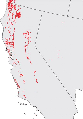
The data specifying the locations of ultramafic rocks (Krevor et al., 2009) was contained within ArcGIS format shapefiles, with California deposits defined by 1071 irregular polygon shapes (Figure 1). Polygon centroids were computed as averages of X, Y values in meters based on the Lambert Conformal Conic Projection. Boundaries and centroids for year 2000 census tracts and counties were obtained from the US Census Bureau (USCB, 2012). They were converted from decimal latitude and longitude to the X, Y coordinate system of the ultramafic rocks using the M map MATLAB toolbox (Pawlowicz, 2011).

Figure 1. Ultramafic rock deposits in California (southern part, truncated in this figure, has no deposits).

Results

This section summarizes the results of analyses designed to explore whether non-causal regression and associations commonly occur in practice, using the spatial data from California as a case study.

Fatal car accidents and proximity to putative asbestos sources (ultramafic rock deposits)

Table 3 shows the results of a multivariate linear regression model for traffic fatality rates (average annual traffic fatalities per 100 000 people per year (1999–2004)) as a function of distances from the five closest ultramafic rock deposits, UM1–UM5.

Table 3. Traffic fatality rates depend on distance from ultramafic rock.

	Regression summary for dependent variable: TRAFFICALL RATE (2000 Data By Extended Tract. R = 0.42525247; R^2= 0.18083966; Adjusted R^2= 0.18025812; F(5,7043) = 310.97; p < 0.0000; Std.Err. of estimate: 59.452)
N = 7049	b*	Std.Err. of b*	b	Std.Err. of b	t(7043)	p Value
Intercept			92.01	1.54	59.6	0.000000
UM1	−0.04	0.07	−0.09	0.15	−0.6	0.562355
UM2	−1.71	0.21	−3.75	0.45	−8.4	0.000000
UM3	2.19	0.24	4.84	0.52	9.3	0.000000
UM4	0.34	0.13	0.76	0.29	2.7	0.008008
UM5	−0.69	0.02	−0.81	0.03	−29.6	0.000000

UM1, UM2, … , UM5 denote the distances between the centroids of census tracts for which data (e.g. on traffic fatality rates) are collected, and the centroids of the closest, second closest, … , fifth closest ultramafic rock deposits, respectively. The linear regression coefficients (determined by ordinary least squares) appear in the b column, and their standardized values in the b* column; in addition, standard errors are shown for both. Values of t tests for these coefficients to be statistically significantly different from zero, and p values for these hypothesis tests appear in the right-most columns of the table, respectively.

Two striking features of Table 3 are that most of the distances from ultramafic rock deposits are highly statistically significant predictors of traffic fatalities (with the exception of UM1, the distance to the closest deposit); and the signs of the relations are both positive (for UM3 and UM4) and negative (for UM2 and UM5). Such highly statistically significant, yet inconsistently directed, associations are precisely what might be expected if the regression model is only revealing random trends in the spatial data, where the signs of the trends differ on different distance scales, e.g. due to random fluctuations in the spatially auto-correlated data.

In the regression models shown in Tables 3–7, the usual regression assumption of statistically independent errors in the dependent values is violated because mortality rates for all tracts in the same county are equal to the county values, reducing the degrees of freedom. (This illustrates the importance of checking regression model diagnostics and testing for model specification errors, neither of which is usually reported in studies such as those in Table 1.) However, the key point that statistically significant-seeming regression coefficients result from applying standard regression procedures to spatial data, even if the assumptions underlying the procedures are not necessarily well justified, remains true, even if only counties, rather than tracts, are used. For example, UM5 remains a statistically significant predictor of traffic mortality rates (b* = −1.45, p = 0.0016) using only county-level data (with n = 47 counties). A companion paper (Berman et al., 2013) further illustrates this point for simulated data, without the constraint that all tracts in the same county have the same county-specific mortality rates. Recognizing that p levels are artificially small when county data are imputed to tracts and the tract data values are then treated as independent observations, we will nonetheless use such imputed data to illustrate key points about the limitations of regression modeling of the data. As noted later, key points can also be illustrated (albeit less vividly) using the county-level data.

Table 4. Multivariate regression model for traffic fatalities within 50 km of ultramafic rock.

	Regression summary for dependent variable: TRAFFICALL RATE, UM1 <50 km; R = 0.51 R2 = 0.26 Adjusted R^2= 0.26
N = 4942	b*	Std.Err. of b*	b	Std.Err. of b	t(4937)	p Value	Valid N
PopDensity	−0.43	0.01	−0.00	0.00	−33.1	0.000000	4948
UM1	−0.09	0.01	−0.37	0.05	−7.0	0.000000	4948
Pop65 + Pov	0.08	0.01	0.14	0.02	6.4	0.000000	4948
pBlueCollar	0.37	0.01	135.94	4.75	28.6	0.000000	4948
Intercept			83.10	2.18	38.1	0.000000

Table 5. Multivariate regression model traffic fatalities within 10 km of ultramafic rock.

	Regression summary for dependent variable: TRAFFICALL RATE R = 0.48; R^2= 0.23; Adjusted R^2= 0.23 Include condition: UM1 < 10 km
N = 1616	b*	Std.Err. of b*	b	Std.Err. of b	t(1611)	p Value
Intercept			52.23	4.31	12.1	0.000000
UM1	0.05	0.02	1.26	0.54	2.3	0.019075
pBlueCollar	0.33	0.02	129.60	8.86	14.6	0.000000
Pop65 + Pov	0.11	0.02	0.19	0.04	4.7	0.000002
PopDensity	−0.33	0.02	−0.00	0.00	−14.1	0.000000

Table 6. Relative risk of Kaposi’s sarcoma (relative to pancreatic cancer) decreases with distance from nearest ultramafic rock deposit (UM1), for UM1 <10 km.

	Regression summary for dependent variable: KS: PANC ratio R = 0.69; R^2= 0.47; Adjusted R^2= 0.475 Include condition: UM1 < 10 km
N = 1616	b*	Std.Err. of b*	b	Std.Err. of b	t(1611)	p Value
Intercept			0.14	0.01	23.1	0.000000
UM1	−0.27	0.02	−0.01	0.00	−14.4	0.000000
pBlueCollar	−0.20	0.02	−0.13	0.01	−10.5	0.000000
Pop65 + Pov	0.10	0.02	0.00	0.00	5.2	0.000000
PopDensity	0.49	0.02	0.00	0.00	25.0	0.000000

Table 7. Relative risk of Kaposi’s sarcoma (relative to pancreatic cancer) increases with distance from nearest ultramafic rock deposit (UM1).

	Regression summary for dependent variable: KS: PANC ratio R = 0.51; R^2= 0.26; Adjusted R^2= 0.26
N = 7049	b*	Std.Err. of b*	b	Std.Err. of b	t(7044)	p Value
Intercept			0.08	0.00	43.1	0.000000
UM1	0.11	0.01	0.00	0.00	10.3	0.000000
pBlueCollar	−0.23	0.01	−0.08	0.00	−21.0	0.000000
Pop65 + Pov	0.06	0.01	0.00	0.00	5.5	0.000000
PopDensity	0.51	0.01	0.00	0.00	47.3	0.000000

Suppose now that, in the imputed tract-level data set, a researcher is convinced that proximity to ultramafic rock is a cause of car accidents, and that the closest source of ultramafic rock should exert a strong effect on car fatalities. How might he use the spatial data to derive apparently strong statistical support for these beliefs? Table 4 shows the result of fitting a multivariate linear regression model to all data from tracts with centroids within 50 km of an ultramafic rock deposit. Within this radius, a highly statistically significant negative regression coefficient relates UM1 to traffic fatalities, suggesting that, the closer a driver is to the nearest source of ultramafic rock, the higher is his risk of a car accident fatality, just as the researcher expected. The other variables in the model include a measure of poverty (“Pop65 + Pov” refers to the fraction of the elderly (over 65) population below the poverty line), population density (“PopDensity,” which helps to indicate urban-rural distinctions), and proportion of population with blue collar jobs (pBlueCollar). These socioeconomic factors are also highly significant predictors of traffic fatality rates. The purpose of this model is not to develop in detail a model for predicting traffic fatality risks; if it were, many other variables, such as median household income, could be added to further improve model fit. Rather, it is to show that it is easy to find multivariate models in which the regression coefficient relating UM1 to traffic accident fatality risks is significantly negative. Table 4 illustrates one such model, and others can easily be generated by including other variables as predictors.

On the other hand, suppose that a different researcher feels equally passionate that proximity to ultramafic rock is beneficial, and that it significantly reduces the risk of car accidents. How might she use the same spatial data to support this opposite conclusion? Table 5 shows the result of fitting a different multivariate linear regression model (for the same variables as in Table 2) to all data from tracts with centroids within 10 km of an ultramafic rock deposit. Within this narrower radius, a statistically significant positive regression coefficient relates UM1 to traffic fatality rates, suggesting that, the closer a driver is to the nearest source of ultramafic rock, the lower is his risk of a car accident fatality. Again, the researcher’s prior expectations appear to be well supported by the data.

Ability to support any desired conclusion (including contradictory ones) by choosing radii of different sizes for the spatial data to include in the analysis appears analogous to the ability, in time series analysis of autocorrelated processes with unit roots (e.g. random walks), to obtain either positive or negative trends, simply by adjusting the length of the interval analyzed (e.g. due to the arcsine law for random walks) (www.encyclopediaofmath.org/index.php/Arcsine_law).

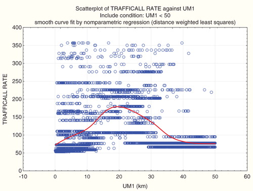
Figure 2 fits a non-parametric smooth regression curve (using a distance-weighted least squares (local polynomial regression) smoothing algorithm, Statistica, 2012) to the proximity-traffic fatality data. The result is a smooth, but clearly non-monotonic, exposure–response relation (using proximity to ultramafic rock as a surrogate for exposure). A parametric (e.g. linear or logistic regression model), which assumes a single coefficient relating UM1 to traffic fatality rates, can produce either a positive average slope or a negative one, depending on what part of the full range of data is included.

Figure 2. Non-parametric regression of traffic fatality rates versus UM1.

Kaposi’s sarcoma and proximity to ultramafic rock deposits

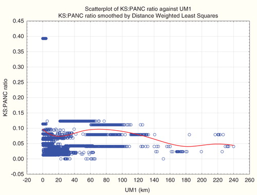
What is true for car accidents is also true for other causes of death: proximity to ultramafic rock is a strong predictor for cause-specific disease incidence. For example, Table 6 shows the results of a multivariate linear regression model for incidence of Kaposi’s sarcoma, a tumor caused by human herpesvirus. Figure 3 shows a smooth exposure–response curve relating risk of Kaposi’s sarcoma to proximity to the closest ultramafic rock deposit (UM1). Tables 6 and 7, inspired by the analysis of Pan et al. (2005), treat the ratio of Kaposi’s sarcoma incidence counts to pancreatic cancer incidence counts as the dependent variable. Again, one can conclude that relative risk of Kaposi’s sarcoma is significantly positively or significantly negatively associated with distance to ultramafic rock (UM1), by selecting an appropriate radius (e.g. infinite or 10 km, respectively). (For county-level data, relative risk of Kaposi’s sarcoma is significantly negatively associated with UM1 if the radius is 30 km.) Again, the non-parametric regression relation (Figure 3) explains this by the fact that there are different average trends on different distance scales – all highly statistically significantly different from zero, for the imputed tract-level data, but with opposite signs at different distances. A curve very similar in shape to Figure 3 describes the absolute risk of Kaposi’s sarcoma, as opposed to its ratio to pancreatic cancer (and absolute risk of Kaposi’s sarcoma is also significantly negatively associated with UM1 in county-level data if the radius is 30 km.).

Figure 3. Non-parametric regression of Kaposi’s sarcoma-to-pancreatic cancer incidence counts ratio (KS:PANC) versus UM1 shows different associations at different distances.

Mesothelioma and proximity to ultramafic rock deposits

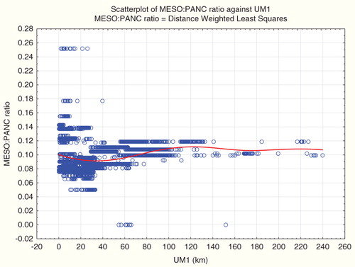
Figures 4 and 5 plot absolute and relative (to pancreatic cancer) mesothelioma incidence risks against distance from ultramafic rock deposits (UM1). Broadly consistent with the observations of Pan et al. (2005) (but without multivariate adjustments), both absolute and relative mesothelioma risks increase with proximity to ultramafic rock on some distance scales. However, the sign of the association reverses on larger distance scales, similar to associations for Kaposi’s sarcoma. Hence, fitting any model with a single regression coefficient to relate UM1 to risk would be misleading, as the sign of their association varies with distance. Spearman’s rank correlation coefficients show that UM1 is significantly positively associated with mesothelioma rate (MESOALL), traffic fatality rate (TRAFICALL RATE) and relative risk of Kaposi’s sarcoma (relative to pancreatic cancer), with about equal strengths (Spearman’s rank correlation between 0.27 and 0.28) for all three. However, Figures 4 and 5 show that the signs of these associations simply reflect where most people live (i.e. at distances with positive rather than negative associations), rather than any underlying consistent positive association. Together, Figures 2–5 show that positive or negative statistical associations of health endpoints with distance from sites reflect where people live and the distance scales chosen for the analysis, rather than consistent underlying positive or negative effects.

Figure 4. Non-parametric regression of mesothelioma rate versus UM1 shows different associations at different distances.

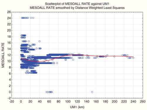
Figure 5. Non-parametric regression of mesothelioma-to-pancreatic cancer incidence count ratio (MESO:PANC) versus UM1 shows different associations at different distances.

Results for point sources

The preceding results use distance to ultramafic rock as an explanatory variable. In California, there are multiple deposits of ultramafic rock, running roughly in two main north-to-south stripes (Figure 2). Thus, the distance to UM can be thought of as (roughly) the distance to the nearer of two line sources on the scale of the state. But many of the studies in Table 1 are for point sources. It is therefore interesting to examine the dependence of other variables on distance from an arbitrary point source. Tables 8–10 choose the centroid of all the census tracts (median latitude and median longitude converted to X,Y) as such a point, and show that distance from this centroid is a statistically significant predictor of both traffic fatality and Kaposi’s sarcoma risk, as well as mesothelioma risk, in the population. The same is true for distance from other arbitrary points, selected at random; and for the ratio of mesothelioma to pancreatic cancer cases. Plotting risk versus distance from a point again yields non-monotonic curves, with different average slopes for different distance scales, similar to what we have already seen for distance from ultramafic rock (e.g. Figure 3).

Table 8. Multivariate model for traffic fatalities versus distance from the centroid of data.

	Regression summary for dependent variable: TRAFFICALL RATE R = 0.51; R^2= 0.26; Adjusted R^2= 0.26
N = 7049	b*	Std.Err. of b*	b	Std.Err. of b	t(7043)	p Value
Intercept			59.04	2.67	22.1	0.000000
UM1	0.08	0.01	0.18	0.02	8.1	0.000000
pBlueCollar	0.35	0.01	129.39	4.03	32.1	0.000000
Pop65 + Pov	0.08	0.01	0.15	0.02	7.9	0.000000
PopDensity	−0.42	0.01	−0.00	0.00	−38.8	0.000000
Distance from centroid	0.09	0.01	5.40	0.64	8.5	0.000000

Table 9. Multivariate model for Kaposi’s sarcoma versus distance from the centroid of data.

	Regression summary for dependent variable: KSALL RATE R = 0.51; R^2= 0.26; Adjusted R^2= 0.26
N = 7049	b*	Std.Err. of b*	b	Std.Err. of b	t(7043)	p Value
Intercept			7.10	0.29	24.5	0.000000
UM1	0.10	0.01	0.02	0.00	10.0	0.000000
pBlueCollar	−0.22	0.01	−8.91	0.44	−20.4	0.000000
Pop65 + Pov	0.06	0.01	0.01	0.00	5.5	0.000000
PopDensity	0.51	0.01	0.00	0.00	47.2	0.000000
Distance from centroid	0.06	0.01	0.39	0.07	5.6	0.000000

Table 10. Multivariate model for mesothelioma versus distance from the centroid of data.

	Regression summary for dependent variable: MESOALL RATE R = 0.37; R^2= 0.14; Adjusted R^2= 0.14
N = 7038	b*	Std.Err. of b*	b	Std.Err. of b	t(7032)	p Value
Intercept			8.85	0.09	103.2	0.000000
UM1	0.15	0.01	0.01	0.00	13.2	0.000000
pBlueCollar	0.04	0.01	0.46	0.13	3.5	0.000423
Pop65 + Pov	−0.03	0.01	−0.00	0.00	−2.6	0.008805
PopDensity	−0.16	0.01	−0.00	0.00	−14.0	0.000000
Distance from centroid	0.29	0.01	0.53	0.02	25.7	0.000000

These findings suggest that discovering a statistically significant regression coefficient linking a health risk variable to proximity to a source (or to multiple sources, as in the ultramafic rock example) should not, by itself, be taken as evidence that the source(s) probably cause or contribute to (or reduce) the health risk.

Theoretical interpretation: what does a spatial regression coefficient show?

The preceding results raise the questions of what does explain observed distance-risk associations, and what the regression coefficients between spatially distributed variables do signify, if not causation. Figure 6 suggests a possible answer. Geographic contours of approximately equal risks for traffic fatalities, here interpolated by fitting a smooth (spline) surface to data on traffic fatalities in tracts with different latitudes and longitudes (for the tract centroids), show that risks tend to increase toward the northeast. (Only the risks contours that fall in the data cloud are empirically driven: the much higher risks to the extreme northeast are just extrapolations of the spatial trends from the limited data. Although more detailed spatial resolution of the data might give different surfaces and contours, our argument is general.) Given such a spatial distribution of risks, choosing any line that runs diagonally through the state from its northwest to its southeast – whether of ultramafic rock or something else – will create a line source with the property that populations to the left and below (southwest of) the line will tend to have smaller risks than populations above and to the right (northeast) of it.

Figure 6. Traffic fatality rates versus latitude and longitude for 7049 California Census tracts (contour view).

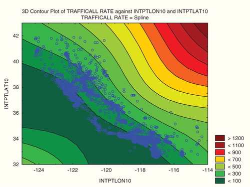
If the population on one side of the line is much bigger than the population on the other side of it, then average risk will change with proximity to the line, simply reflecting the fact that risk generally decreases from the northeast to the southwest, even if the line itself (or sources located along it) have no effect on risk. Similarly, if one selects a point at random, and if population is not symmetrically distributed around it, then people living near the point may tend to be on a higher or lower contour (depending on the location of the point) than most of the population that lives far from it. (To see this, pick a point at random in Figure 6, and confirm that nearest neighbors will, in most cases, live on different risk contours from those who live far away.) Therefore, what a regression coefficient of risk versus distance indicates is not necessarily a causal effect of distance on risk, but rather a reflection of the spatial distribution of the population over risk contours. Thus, the results of studies such as that of Pan et al. (2005) and others in Table 1, which present regression coefficients without modeling the non-causal effects of such spatial distributions of populations, do not provide a reliable basis for drawing causal inferences.

Discussion and conclusions

This paper has examined whether non-causal spatial regression relations arise in realistic data sets when proximity to ultramafic rock is used as an exposure surrogate and various outcomes (traffic fatality rate, absolute risk of Kaposi’s sarcoma, and relative risk of Kaposi’s sarcoma and mesothelioma (both compared to pancreatic cancer)) are treated as response variables. The main finding is that statistically significant associations can readily be found in multivariate linear regression models (as well as in univariate linear and non-parametric regression analyses), although the signs of the associations depend on the distance scales considered. These include causally implausible associations (e.g. between distance from ultramafic rock and traffic fatality or Kaposi’s sarcoma risks) as well as more causally plausible ones (e.g. between distance from ultramafic rock and mesothelioma risks). Such associations serve as negative controls (Lipsitch et al., 2010), indicating that the associations are likely to reflect bias or confounding, rather than purely causal effects.

Of course, none of these statistical associations should be interpreted as demonstrating that proximity to geological features either causes or protects against car accident fatalities, sexually transmitted diseases or other health outcomes. A plausible alternative hypothesis is that spatial location acts as a confounder when there are spatial trends in both explanatory and dependent variables. Such trends can arise even in random spatial autoregressive processes (Lauridsen & Kosfeld, 2011), although here we have focused on real-world trends arising from the specific population distribution in California. Such spatial trends in both exposure and response variables create highly statistically significant exposure–response regression coefficients, whether or not there is any causal relation between them.

For spatial ecological studies such as those in Table 1, traditional methodological concerns about ecological associations also apply. For example, multiple testing and confirmation biases (Sarewitz, 2012) can produce excess false positives if investigators must make numerous modeling choices (e.g. of which confounders, covariates and interactions to include in the model; what model forms to specify; how to treat exposure uncertainties, and so forth). Such concerns are addressed in a companion paper (Berman et al., 2013) via simulation modeling, where the underlying data-generating process is exactly known. Yet, the types of phenomena noted here (non-causal associations reflecting the underlying spatial distributions of variables) still arise. That even highly significant regression coefficients for health effects versus proximity to sources may simply reflect the spatial distribution of a population, rather than an effect of proximity on health effects, adds to these traditional concerns. In addition, future experimental investigation might greatly clarify causality, e.g. by revealing whether measured concentrations in air of mineral products from ultramafic rock deposits are capable of causing changes in the lung environment (e.g. inflammation, increases in oxidative stress) of potential importance in the etiology of mesothelioma (e.g. Carbone & Yang, 2012). This paper has focused on causal interpretation of regression coefficients in observational (and ecological) data. Experimental and toxicological investigations could potentially provide a different basis for understanding whether causal interpretations of such associations is likely to be warranted. Meanwhile, our findings suggest that such additional insights would be valuable before causal interpretations of associations are acted on, since statistically significant associations commonly occur in regression analyses of observational data with spatially distributed variables, even when there are no known plausible causal relations between exposure and effect variables.

These findings suggest that extreme caution is needed in interpreting the conclusions from studies such as those in Table 1. Unless it is demonstrated that proximity–response associations are not explained by non-causal artifacts of spatial regression (e.g. spurious regression), using appropriate spatial statistical tests (e.g. Lauridsen & Kosfeld, 2011) and also that they are not due to model-specification errors (e.g. attempting to fit regression models with constant coefficients to relations that are non-monotonic), the presence of positive regression coefficients should not be interpreted as providing any evidence for a true exposure–response relation. Our findings (as well as those in Berman et al., 2013) suggest that such regression relations may be ubiquitous in realistic spatial epidemiological data, even when no causal interpretation is plausible. Additional analyses, analogous to those in Table 2, are therefore likely to become recognized as essential preludes to valid causal interpretation of spatial exposure–response associations.

Declaration of Interest

The authors thank the National Stone, Sand, and Gravel Association (NSSGA) for a grant that provided partial support for the research reported here and the writing of this paper. The authors consult for a variety of government and private organizations with competing interests; none was involved in this work. NSSGA had no input into the work. The research questions addressed, methods applied, analyses conducted and conclusions drawn are solely those of the authors.

References

- Angrist JD, Pischke J-S. (2009). Mostly harmless econometrics: an empiricist’s companion. Princeton, NJ: Princeton University Press
- Berman DW, Cox, T, Popken, D. (2013). A cautionary tale: the characteristics of two-dimensional distributions and their effects on epidemiological studies employing an ecological design. Crit Rev Toxicol (this supplement)
- CCR (California Cancer Registry). (2012). Cancer incidence/mortality rates in California. Available from http://www.cancer-rates.info/ca [last accessed 5 Jan 2012]
- Campbell DT, Stanley JC. (1966). Experimental and quasi-experimental designs for research. Chicago: Rand McNally
- Carbone M, Yang H. (2012). Molecular pathways: targeting mechanisms of asbestos and erionite carcinogenesis in mesothelioma. Clin Cancer Res, 18, 598–604
- Cox Jr LA. (2007). Regulatory false positives: true, false, or uncertain? Risk Anal, 27, 1083–6
- Cox T, Popken D, Ricci PF. (2013). Temperature, not fine particulate matter (PM2.5), is causally associated with short-term acute daily mortality rates: results from one hundred United States cities. Dose-Response. Available from: http://dose-response.metapress.com/media/n0fdjqeyyrcrvw9xjywv/contributions/n/4/n/5/n4n550pp25557670.pdf [last accessed 18 March 2013]
- CSDC (California State Data Center). (2012). Selected census 1990 and 2000 population and housing estimates for tract 2000. California Dept. of Finance, Demographic Research Unit, California State Data Center. Available from: http://www.dof.ca.gov/research/demographic/state_census_data_center/products-services/ [last accessed 5 Jan 2012]
- Dash D, Druzdzel MJ. (2008). A note on the correctness of the causal ordering algorithm. Artif Intell, 172, 1800–8
- Druzdzel MJ, Simon HA. (1993). Causality in Bayesian belief networks. Proceedings of the Ninth Annual Conference on Uncertainty in Artificial Intelligence (UAI-93), The Catholic University of America, Providence, Washington, DC, USA, July 9–11. San Francisco, CA: Morgan Kaufmann Publishers, Inc., 3–11. Available from: http://www.informatik.uni-trier.de/∼ley/db/conf/uai/uai1993.html [last accessed 23 March 2013]
- Eichler M, Didelez V. (2010). On Granger causality and the effect of interventions in time series. Lifetime Data Anal, 16, 3–32
- Freedman DA. (2004). Graphical models for causation, and the identification problem. Eval Rev, 28, 267–93
- Friedman N, Goldszmidt M. (1998). Learning Bayesian networks with local structure. In: Jordan MI, ed. Learning in graphical models. Cambridge, MA: MIT Press, 421–59
- García-Pérez J, Pollán M, Boldo E, Pérez-Gómez B, et al. (2009). Mortality due to lung, laryngeal and bladder cancer in towns lying in the vicinity of combustion installations. Sci Total Environ, 407, 2593–602
- García-Pérez J, López-Cima MF, Boldo E, et al. (2010). Leukemia-related mortality in towns lying in the vicinity of metal production andprocessing installations. Environ Int, 36, 746–53
- Gardner, D. (2009). The science of fear: how the culture of fear manipulates your brain. New York: Penguin Group
- Gilmour S, Degenhardt L, Hall W, Day C. (2006). Using intervention time series analyses to assess the effects of imperfectly identifiable natural events: a general method and example. BMC Med Res Methodol, 6, 16. Available from: http://www.biomedcentral.com/1471-2288/6/16 [last accessed 23 Mar 2013]
- Goria S, Daniau C, de Crouy-Chanel P, et al. (2009). Risk of cancer in the vicinity of municipal solid waste incinerators: importance of using a flexible modeling strategy. Int J Health Geogr, 8, 31. Available from: http://www.ij-healthgeographics.com/content/8/1/31 [last accessed 23 Mar 2013]
- Hack CE, Haber LT, Maier A, et al. (2010). A Bayesian network model for biomarker-based dose response. Risk Anal, 30, 1037–51
- Helfenstein U. (1991). The use of transfer function models, intervention analysis and related time series methods in epidemiology. Int J Epidemiol, 20, 808–15
- Imberger G, Vejlby AD, Hansen SB, et al. (2011). Statistical multiplicity in systematic reviews of anaesthesia interventions: a quantification and comparison between Cochrane and non-Cochrane reviews. PLoS ONE, 6, e28422. Available from: http://www.ncbi.nlm.nih.gov/pubmed/16060722 [last accessed 23 Mar 2013]
- Ioannidis JPA. (2005). Why most published research findings are false. PLoS Med, 2, e124
- Krevor SC, Graves CR, Van Gosen BS, McCafferty AE. (2009). Mapping the mineral resource base for mineral carbon-dioxide sequestration in the conterminous United States: U.S. Geological Survey Digital Data Series 414. Available from: http://pubs.usgs.gov/ds/414/
- Lauridsen J, Kosfeld R. (2011). Spurious spatial regression and heteroscedasticity. J Spatial Sci, 56, 59–72
- Lehrer J. (2012). Trials and errors: why science is failing us. Wired. Available from: http://www.wired.co.uk/magazine/archive/2012/02/features/trials-and-errors?page=all [last accessed 28 Jan 2012]
- Lipsitch M, Tchetgen Tchetgen E, Cohen T. (2010). Negative controls: a tool for detecting confounding and bias in observational studies. Epidemiology, 21, 383–8
- López-Abente G, Fernández-Navarro P, Boldo E, et al. (2012). Industrial pollution and pleural cancer mortality in Spain. Sci Total Environ, 424, 57–62
- Loyo-Berríos NI, Irizarry R, Hennessey JG, et al. (2007). Air pollution sources and childhood asthma attacks in Catano, Puerto Rico. Am J Epidemiol, 165, 927–35
- Maclure M. (1990). Multivariate refutation of aetiological hypotheses in non-experimental epidemiology. Int J Epidemiol, 19, 782–7
- Monge-Corella S, García-Pérez J, Aragonés N, et al. (2008). Lung cancer mortality in towns near paper, pulp and board industries in Spain: a point source pollution study. BMC Public Health, 8, 288. Available from: http://www.ncbi.nlm.nih.gov/pmc/articles/PMC2527328/ [last accessed 23 Mar 2013]
- Moore KL, Neugebauer R, van der Laan MJ, Tager IB. (2012). Causal inference in epidemiological studies with strong confounding. Stat Med, 31, 1380–404
- NHTSA (National Highway Traffic and Safety Administration). (2012). Fatality analysis reporting system. Available from: http://www-fars.nhtsa.dot.gov/Main/index.aspx [last accessed 5 Jan 2012]
- Ottenbacher KJ. (1998). Quantitative evaluation of multiplicity in epidemiology and public health research. Am J Epidemiol, 147, 615–619
- Pan XL, Day HW, Wang W, et al. (2005). Residential proximity to naturally occurring asbestos and mesothelioma risk in California. Am J Respir Crit Care Med, 172, 1019–25
- Pawlowicz, R. (2011). M_Map: a mapping package for MATLAB. Avaialble from: http://www2.ocgy.ubc.ca/~rich/map.html [last accessed 5 Jan 2012]
- Ramis R, Diggle P, Cambra K, López-Abente G. (2011). Prostate cancer and industrial pollution: risk around putative focus in a multi-source scenario. Environ Int, 37, 577–85
- Robins JM, Hernán MA, Brumback B. (2000). Marginal structural models and causal inference in epidemiology. Epidemiology, 11, 550–60
- Sarewitz D. (2012). Beware the creeping cracks of bias. Nature, 485, 149
- Statistica. (2012). Statistica 10 documentation. Available from: http://documentation.statsoft.com/STATISTICAHelp.aspx?path=Graphs/Graph/ModifyingGraphs/Notes/DistanceWeightedLeastSquaresFitting [last accessed 18 March 2013]
- Stebbings Jr JH. (1978). Panel studies of acute health effects of air pollution. II. A methodologic study of linear regression analysis of asthma panel data. Environ Res, 17, 10–32
- USCB (U.S. Census Bureau). Census 2000 TIGER/Line Files. Available from: http://www.census.gov/geo/www/tiger/tiger2k/tgr2000.html [last accessed 5 Jan 2012]