An “optimal” k-needle placement strategy and its application to guiding transbronchial needle aspirations

Abstract

This article addresses the problem of finding an “optimal” strategy for placing k biopsy needles, given a large number of possible initial needle positions. We consider two variations of the problem: (1) Calculate the smallest set of needles necessary to guarantee a successful biopsy; and (2) Given a number k, calculate k needles such that the probability of a successful biopsy is maximized. Note that “needle” is used as shorthand for the parameter vector that specifies the needle placement. Both problems are formulated in terms of two general, NP-hard optimization problems. Our k-needle placement strategy can be considered as “optimal” in the sense that we are able to formulate it as a known NP-hard problem for which it is believed (NP≠P conjecture) that no efficient algorithm exists that computes the optimal solution. In other words, our strategy is “optimal” with respect to the best approximative algorithm known for the respective NP-hard problem. For the second variation we have implemented an approximative algorithm that is guaranteed to be within a factor of≈0.63 of the exact solution. Given a number k, the algorithm calculates k sets of parameters, each set specifying the placement of a needle and the corresponding probability of success. The resulting probabilities show that our approach can provide valuable decision support for the physician in choosing how many needles to place and how to place them.

A typical example of a biopsy where the initial needle position is known approximately is a transbronchial needle aspiration (TBNA). We demonstrate how our “optimal” needle placement strategy can be used to achieve sensor-less guidance of TBNA. The basic idea is to use a patient-specific model of the tracheobronchial tree (from CT/MR) and our model for flexible endoscopes to preoperatively estimate the unknown position of the bronchoscope. The result is a set of candidate shapes for the unknown shape of the bronchoscope before needle placement or, in other words, a (large) number of possible initial needle positions. By parameterizing the handling of the bronchoscope, including the insertion of the biopsy needle, we are able to apply our “optimal” strategy. The result is a TBNA protocol that, if executed during the procedure, prescribes how to handle the bronchoscope to maneuver the needle into the target. With the aforementioned endoscope model, we present a new way of modeling long, flexible instruments. The algorithm requires no initialization or preprocessing and calculates the workspace of an instrument based on its insertion depth and a set of internal and external constraints.

• Bronchoscopy
• needle biopsy
• transbronchial needle aspiration
• TBNA
• endoscope model
• set-covering problem
• virtual endoscopy

Introduction

A biopsy is a minimally invasive surgical procedure, often used in the diagnosis and staging of cancer patients. In general, the goal is to sample the suspicious tissue (the target) by placing a biopsy needle inside it. Since the target is often not directly visible to the physician, numerous methods for guiding biopsies have been developed. Procedures that have attracted special attention in recent years include biopsy of the prostate, breast, liver and lung.

In many cases it is common practice to collect more than one tissue sample to increase the probability of hitting the target. Instead of using a simple trial-and-error approach, biopsy strategies have been developed for, among others, prostate cancer biopsies [1], [2]. The k-Needle Placement Strategy is a biopsy protocol that specifies how to place k (biopsy) needles, such that the probability of success is maximized. The placement of a needle is specified by a suitable parameterization of its degrees of freedom, e.g., by two angles and an insertion depth.

This article presents an “optimal” strategy for placing k biopsy needles for a class of biopsy problems where the target is known exactly but the initial needle position is only known approximately. In a discrete sense, knowing the initial needle position approximately can be formulated as having been given a (large) number of possible initial needle positions. It is assumed that each possible initial needle position has the same probability of being the actual (however unknown) position of the needle before placement. For a sufficiently small number of initial needle positions (e.g., three), the problem becomes trivial: Simply calculate for each initial needle position the parameters that specify how to maneuver the needle into the target. In this unrealistic scenario, each possible initial needle position is “covered” by the placement of one needle. Note that we use “needle” as shorthand for the parameter vector that specifies the needle placement. For a large number of initial needle positions, finding an optimal strategy translates to finding a placement strategy that covers the initial needle positions as well as possible. More specifically, we consider two definitions of the term “optimal strategy”: (1) A placement strategy for k needles is optimal if it covers all initial needle positions and no strategy using less than k needles guarantees the same; (2) Given a number k, a placement strategy for k needles is optimal if no other k-needle placement strategy covers more initial needle positions. The key observation is that the more initial needle positions are covered by a k-needle strategy, the higher the probability that the actual needle position is covered, and the higher the probability that one of the k needles hits the target.

These two variations can also be formulated as: (1) Calculate the smallest set of needles necessary to guarantee a successful biopsy; and (2) Given a number k, calculate k needles such that the probability of a successful biopsy is maximized. We provide a solution to both problems by formulating them in terms of two general, NP-hard optimization problems.

We consider our k-needle placement strategy to be “optimal” in the sense that we are able to formulate it as a known NP-hard problem for which it is believed (NP≠P conjecture) that no efficient algorithm exists to compute the optimal solution. In other words, our strategy is “optimal” with respect to the best approximative algorithm known for the respective NP-hard problem. For the latter problem there exists an approximative algorithm which requires virtually no implementation effort and is guaranteed to be within a factor of 1−1/e≈0.63 of the exact solution. For both variations of the problem, success probabilities for each needle are provided to the physician.

A typical example of a procedure where the initial needle position is known approximately is a transbronchial needle aspiration (TBNA) biopsy [3]. Traditionally, this biopsy is performed by maneuvering a bronchoscope to a suitable site within the tracheobronchial tree. The bronchoscopist then inserts a needle through the bronchoscope and punctures the bronchial wall to hit the target lying behind. TBNA is a valuable, minimally invasive procedure with an often-positive outcome for the patient. In contrast to open surgery for this purpose, TBNA is an outpatient procedure. Unfortunately, only a few bronchoscopists routinely perform TBNA, since the “blind” puncture requires considerable skill and experience.

For this reason, several methods for guiding TBNA have been proposed. They can be classified into three categories: imaging-based, vision-based and sensor-based approaches. In the imaging-based category, standard real-time imaging technology, such as conventional fluoroscopy, CT-fluoroscopy, CT imaging and ultrasonography is used for TBNA guidance. Approaches in the sensor-based category attach real-time position sensors to the bronchoscope. Finally, vision-based approaches analyze the video images from the CCD camera inside the bronchoscope tip for TBNA guidance. While approaches in the first category try to achieve guidance by directly visualizing the needle/target, approaches in the latter two categories regard the task of guiding TBNA as an application of a more general technique: the continuous tracking of the endoscope tip. Knowing at any point in time the position and viewing direction of the endoscopic camera enables the camera to be registered with a corresponding virtual view. This allows superimposition of structures from a 3D dataset (CT, MR) onto the real endoscopic image, generating the impression of “X-ray vision”.

A subsequent section reviews the literature concerning approaches in each category. Several groups have reported clinical studies of imaging-based approaches, and one group has reported two clinical studies of a sensor-based approach, but there has been no clinical study of a vision-based approach. Although clinically useful, imaging- and sensor-based techniques can generally be considered as being elaborate (relying on expensive, special-purpose devices), cumbersome or time-consuming. On the other hand, vision-based approaches are generally less elaborate but insufficiently reliable or fast to be considered as a mature technique for guiding TBNA. Furthermore, even with “X-ray vision”, the bronchoscopist is still left with the task of actually maneuvering the needle into the target. What is missing is a dedicated solution for guiding TBNA that is fast and easy to set up, is inexpensive, allows for real-time guidance, and supports the bronchoscopist directly in maneuvering the biopsy needle into the target.

This work presents a new paradigm for guiding TBNA, which can be denoted as a model-based approach. It represents a dedicated solution that abandons the idea of continuous tracking of the endoscope tip and supports the bronchoscopist directly in maneuvering the biopsy needle into the target lesion. The basic idea is to calculate a TBNA protocol prior to the intervention. This protocol describes in detail how to perform a series of tissue samplings, by prescribing for each sample how to handle the bronchoscope in order to move the biopsy needle into the target lesion. By using the results of the proposed “optimal” k-needle placement strategy, the protocol gives probabilities of success for each tissue sample. This allows the bronchoscopist to decide whether or not the potential gain from an additional biopsy justifies the associated discomfort and risk for the patient. During the TBNA procedure, the bronchoscopist executes the protocol by setting the bronchoscope to the prescribed configuration. To gain control over the current configuration of the bronchoscope, a set of passive controls is used to monitor its degrees of freedom. The use of passive controls requires no computers or other electronic devices in the operating room.

To calculate the protocol, the handling of the endoscope is parameterized. This set of parameters is called an endoscope configuration. The problem of guiding TBNA can then be formulated as the problem of estimating a set of configurations that together maximize the probability of a successful biopsy. The parameter estimation is based on a patient-specific model of the anatomy (derived from CT/MR) and a model of a flexible endoscope that takes the real endoscope's physical and mechanical properties into account. The endoscope model calculates the real endoscope's workspace, given a set of internal and external constraints. The workspace can be regarded as a set of candidate shapes for the (unknown) shape of the real endoscope. Having a set of candidate shapes can also be interpreted as knowing the position of the real endoscope approximately, which represents the initial condition of the “optimal” k-needle placement strategy.

The outline of this paper is as follows: The next section describes an “optimal” needle placement strategy given an approximate initial needle position. The basic idea is formulated in a generic and abstract way, avoiding any reference to possible applications. The subsequent section describes a specific application of the techniques presented in the preceding section: a model-based approach to guiding TBNA. The centerpiece of this application is a deformable model for long, flexible instruments such as catheters or endoscopes. This section describes how to calculate a detailed protocol for performing TBNAs based on the flexible instrument model and the needle placement strategy described previously. This is followed by a description of experiments and results for the respective ideas introduced in the earlier sections, and the article ends with a discussion of these results and a conclusion.

An “optimal” needle placement strategy given an approximate initial needle position

The following gives a formal description of the problem and presents a “naive” solution. Based on the shortcomings of this approach, the problem is formulated as an optimization problem. A solution to the two variations (see above) of this optimization problem is found by considering a dual problem in the needle parameter domain. The first variation is formulated as the Set-Covering Problem, the second as the Maximum k-Coverage Problem, both classic NP-hard optimization problems. For the first variation, the result is an algorithm that finds, for a given set of possible initial needle positions, the smallest set of needles necessary to guarantee a successful biopsy. For the second variation, the result is an algorithm that maximizes the coverage of the possible initial positions for a given maximum number of k-needles. An experiment based on an approximative algorithm for the second variation, incorporating results from the following section, is described later in the paper.

Problem definition

This section introduces the main components of the problem of finding an “optimal” k-needle placement strategy, given an approximate initial needle position. First, a list of general assumptions is given, then a straightforward solution to the problem is presented and its shortcomings analyzed. They represent the motivation for the following section to formulate the problem as an optimization problem.

Assumptions

The problem is based on the following three assumptions.

1. There exists an initial position domain P, which is a set of possible initial locations for the endoscope before needle placement. Each location has the same probability of being the actual position of the endoscope at the time of needle placement. The endoscope is assumed to be given by the model described in the next section, namely by a sequence of links interconnected by joints. The endoscope's first bending section link can be assumed to remain stationary during the alignment of the tip with a target (active tip deflection). Therefore, this link alone is sufficient to describe the endoscope's initial position before needle placement. In other words, each initial position p∈P can be represented by a single 4×4 matrix (see p. 273, left). Let p̃∈P denote the real but unknown position of the endoscope after insertion. It is assumed that p̃ does not change during needle placement.

2. There exists a target domain T⊂IR³.

3. There exists a function f: P×T→N, which computes for a given p∈P and t∈T the necessary needle parameter n∈N to hit t from position p. N⊂IR³ is denoted as the needle parameter domain. Function f() represents a model for the process of maneuvering the needle into the target. If a link is given by a matrix F, function f() can be written asThis computes the necessary shaft rotation α, needle of tip deflection β, and needle length d (see p. 276, right) to hit a target t∈T from an initial endoscope position p, described by a single link F.

There also exists a dual function f¯ : P×N→IR³, which computes, for a given position p and a needle parameter n, the resulting position of the needle tip. Given function f(), the realization of f¯() is straightforward. Note that the co-domain of f¯() is IR³ (and not T), because for p≠q:Given these assumptions, the k-needle placement problem is to determine a set N_*⊂N of k needle parameters, such that P is covered as well as possible. In the remainder of this section, three such sets N* and their corresponding sets P* in the position domain P are considered:

Definition 1

[N_{{naive, better, opt}} and P_{{naive, better, opt}}]

Let

be subsets of the needle parameter domain N. Then the corresponding sets in the position domain P are denoted byand defined as:Set P_i is the set of all p∈P that are mapped into the target by a needle of set N_i.

Naive method

The following describes a naive solution to the problem of finding a k-needle placement strategy, given an approximate initial needle position. A naive method to find k needle parameters that cover P, is to first select a set P ^Δ of k samples from P. For each sample p_i,∈P ^Δ a needle parameter is calculated that would bring the needle tip into the center of the target:

Note that this abbreviated notation is used as an equivalent for:

In other words, N_naive is a set of needle parameters that hit the target from at least all positions p∈P^Δ. It is hoped that N_naive maps as many p∈P into the target as possible. This strategy has at least two shortcomings. The first of these is that P is not necessarily well covered:

It is not guaranteed that for all endoscope positions p∈P there exists a needle in N_naive, which hits the target. Secondly, N_naive is not necessarily mininal; there may exist a set N_better⊂N such that

P_better covers at least as much of P as P_naive, while needing fewer needles.

These observations suggest the formulation of the k-needle placement problem as an optimization problem.

An “optimal” strategy

In this section, a solution to the problem of finding an “optimal” k-needle placement strategy is developed. We assume that each initial needle position has the same probability of being the actual position of the needle before placement. Then, finding an optimal strategy translates to finding needles that “cover” as many of the initial needle positions as possible. A needle “covers” an area if the same needle parameters, executed from every endoscope position within this area, hit the target. One goal is to solve the problem of minimizing the number of needles needed for a full coverage. The problem of finding the smallest set of needles that cover all initial positions is formulated as the problem of finding the minimum set cover in the needle parameter domain. This problem in turn, can be directly formulated as the Set Covering Problem, a well-known NP-hard optimization problem.

Another goal is to maximize the number of initial positions covered by a given number of k needles. This problem is formulated as the Maximum k-Coverage Problem, likewise an NP-hard, general optimization problem.

Formulation as an optimization problem

An “optimal” k-needle placement strategy is a set N_opt⊂N of needle parameters, such that

In other words, for all endoscope positions p∈P there exists a needle in N_opt that hits the target, and no set smaller than N_opt guarantees the same.

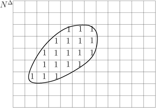
Similar to Definition 1, let P_i denote the set of all p∈P that are mapped into the target by a needle parameter n _i∈N_opt. By definition, N_opt induces a coverage of P by k subsets P_i.

Figure 1 shows an example for k=5. It shows five subsets P₁, … , P₅, with each P_i induced by a needle parameter n _i∈N_opt. This example makes it clear that any given real initial endoscope position p̃ will fall inside a subset P_i and a corresponding needle parameter n_i will map p̃ inside the target. Since p̃ is unknown, all five needle parameters have to be tested, one at a time. In this example, the first, second, fourth and fifth needles will fail and the third will hit the target.

Figure 1 Set P divided into subsets P_i, induced by N_opt. [Color version available online]

The basic idea behind finding the smallest set of subsets in P is to consider a dual problem in the needle parameter domain N. The problem is transformed into N by sampling P and calculating a “scan” of target T from the “perspective” of each sample. The dual problem is then to find a minimum number of points in N such that each scan covers at least one point. This set of points is equivalent to N_opt.

Transformation into the needle parameter domain

For this purpose, the following definition is used:

Definition 2

[S^T(p)] S^T(p) denotes a “scan” of T from a given position p∈P:

S^T(p)⊂N is the set of all needle parameters needed to hit all t∈T from a fixed p. Position p is called the “viewpoint” of the scan.

Figure 2 makes it clear that S^T(p) is the result of T scanned from viewpoint p and that it forms a point cloud in the needle parameter domain.

Figure 2 A “scan” of T from viewpoint p: S^T(p). [Color version available online]

Let target T be discretized into T^Δ, which consists of voxels or cells of side-length Δ_T. A discretization of T also requires a discretization of N in the sense that two needle parameters which map a position p∈P into the same voxel of T^Δ can be regarded as a single needle parameter.

Definition 3

[N^Δ] The needle parameter domain N is discretized into cells. The centers of all cells represent the discretized needle parameter domain N^Δ. Cell size Δ_N is derived from the cell size Δ_T in T^Δ. Let d() be the Euclidian distance:

In the following, the transition is made from S^T(p)⊂N to S^TΔ(p)⊂N^Δ, where S^TΔ(p) is the scan of T^Δ from viewpoint p∈P. The idea is to “round” each n∈S^TΔ(p) to the center of the cell it falls in. If one or more n falls into the same cell, we say the cell is “covered” by the scan. Consequently, it is sufficient to store for each cell the viewpoint p of the scan, which “covers” the cell. This yields the following:

Definition 4

[ and V_i] Each cell of N^Δ stores two pieces of information:

1. ∈N^Δ, the center of cell i,

2. V_i⊆P, the set of viewpoints of cell i.

The “center of cell i” is the needle parameter in the center of cell i. Set V_i is the set of viewpoints of all scans that cover cell i.

Figure 3 shows N^Δ divided into cells and a scan S^TΔ(p₁). For each cell the set of viewpoints V_i is given. The set is either {1} (subscript of viewpoint p₁) if the cell is covered by the scan, or the empty set {} if the cell is not covered.

Figure 3 A scan S^TΔ(p₁) in N^Δ. Each cell shows its set of viewpoints V_i (subscript of p₁ only).

To transform the problem from P to N^Δ, P is sampled and a scan S^TΔ(p_i) is calculated for each p_i∈P. Figure 4 shows an example for three samples, p₁, p₂, and p₃. Each cell's set of viewpoints V_i is given. Note that one cell (boxed) is covered by all three scans. With the center of this cell, this can be interpreted as

Figure 4 Three scans from viewpoint p₁, p₂, p₃. Set V_i of cell i gives the indices of the viewpoints, whose scans cover cell i. Only one cell (boxed) is covered by all three scans.

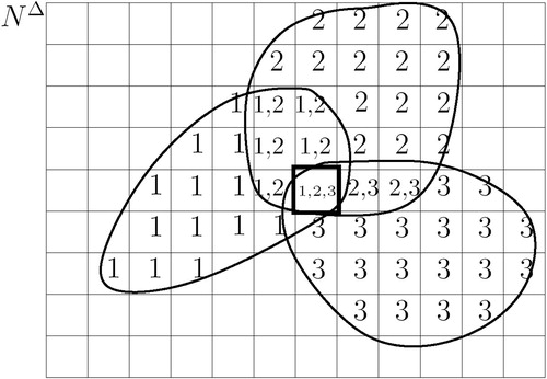
In other words, only needle parameter is required to map all three positions into the target. Positions p₁, p₂, p₃ are members of the same subset, induced by . The goal of dividing P into a minimum number of subsets can now be formulated as the problem of selecting a minimum number of cells in N^Δ, such that each scan covers at least one selected cell. This problem is reduced to the following “classic” optimization problem.

Set covering problem and maximum k-coverage problem

The Set Covering Problem (SCP) is a well known NP-hard combinatorial optimization problem, which can be formulated as follows:

A finite set U of elements and a class S of subsets of U is given. Let S_i denote the i^th subset in S. The task is to select subsets S_i, such that every element in U belongs to at least one S_i. A selection W⊆S with this property is called a set cover of U with respect to S.

The optimization problem is to find a set cover W of minimum cardinality:

The SCP is a subject of numerous publications in the operations research and mathematical literature. Many applications of the SCP to real-world problems, such as resource allocation and scheduling have been described. Exact solutions for modestly sized problems using a dual heuristic have been reported by Fisher and Kedia [4]. For large problems, approximative schemes have been suggested by Beasley [5].

An interesting variation of the SCP is the Maximum k-Coverage Problem (kCP), which can be formulated as follows:

A set U and a class of subsets S is given, as in the SCP, as well as an integer k. Each element u∈U has an associated weight w(u). The optimization problem is to select k subsets S_i from S, such that the weight of the elements in is maximized.

Hochbaum and Pathria [6] have shown that the greedy approach to this NP-hard problem, which at each stage selects the subset giving maximum improvement, is guaranteed to be within a factor of 1 – (1 – 1/k)^k>1 – 1/e of the optimal solution.

Formulation of the problem as an SCP and kCP

The connection between our problem and the SCP can be established as follows:

Let P^Δ be a set of samples of P, V_i⊆P^Δ the set of viewpoints of cell i, and W an arbitrary minimal set cover:

Let ∈N^Δ be the needle parameter in the center of cell i. Then, an “optimal” k-needle placement strategy is given by:

The P_opt=P condition of Equation 7 follows from the SCP condition that every element in U belongs to at least one selected subset S_i. The “|N_opt|=minimal” condition follows from the minimization of the set covers' cardinality.

For example, given the situation shown in Figure 4, U={p₁, p₂, p₃}, S={{},{p₁},{p₂},{p₃}, {p₁,p₂}, {p₂,p₃},{p₁,p₂,p₃}}, W={{p₁,p₂,p₃}} and N_opt={}, where i is the boxed cell.

With this formulation, a subset of P, induced by an ∈N_opt is given by V_i. It is important to note that the quality of solution N_opt depends on the sample density of P^Δ. The connection between our problem and the kCP follows directly from the above theorem, with the weight function given by w(u)=1, for all u∈U. This weight function favors cells that are covered by many scans, since the kCP maximizes the sum of the weights of all elements of all selected subsets.

The kCP is an interesting variation for two reasons: First, the greedy approach is easy to implement by simply selecting at each stage the cell with the highest cardinality of V_i and subsequently updating all V_i. Second, as shown by Hochbaum et al. [6] for small k, a greedily constructed solution is within an acceptable factor from the exact solution. For example, for k<3 the factor is>0.7.

The needle parameters given by N_opt should be executed in order of decreasing probability of success. Regarding a chosen sample density, the probability of hitting target T with a needle parameter ∈N_opt is given by |V_i|/|P^Δ|.

Application to guiding TBNA

The previous section presented in a generic and abstract way an “optimal” k-needle placement strategy for a special class of biopsy problems, where the initial needle position is known approximately. This section presents a clinical example for such a problem and describes how the results from the preceding section can be applied to obtain a solution.

Lung cancer is the leading cause of cancer death in the US and throughout the world. The prognosis for the patient depends on the extent of the disease at the time of diagnosis. For early detection of lung cancer, a low-dose chest CT scan has been used as a screening test. Preliminary results suggest that this may lead to early detection of lung cancer in certain populations and may therefore significantly improve patients' survival rate.

One of the most common radiological findings in lung cancer screening examinations is a solitary pulmonary nodule. It is characterized as a single well-defined, round or oval lesion within the lung up to 6 cm in diameter. Following detection, the nodule has to be classified as benign or malignant. To assess the extent of the disease (staging – see reference [7]) or to establish a ground truth, a tissue sample must be acquired for histological classification of the cell type. This can be done by inserting a needle from the outside directly into the suspect lesion, but this may cause pneumothorax, a serious condition in which air enters the intrapleural space. An alternative, more elegant way that avoids the risk of pneumothorax is transbronchial needle aspiration (TBNA) [8].

TBNA is a valuable minimal invasive procedure in the bronchoscopic diagnosis and staging of patients with lung cancer. The procedure allows nonsurgical access to mediastinal and hilar lymph nodes from inside the tracheobronchial tree. Traditionally, this biopsy is performed by maneuvering a bronchoscope to a suitable site within the tracheobronchial tree. The surgeon then inserts a needle through the bronchoscope and punctures the bronchial wall to hit the target behind it. This is literally a “blind” puncture since the target object is at no time visible through the bronchoscope. The relatively blind nature of the procedure and the physician's lack of confidence regarding positioning of the needle are obstacles to the widespread use and positive diagnostic yield of TBNA. In a 1991 survey [9], only 11.8% of experienced bronchoscopists routinely performed TBNA. The lack of direct sight and tactile feedback, together with the complicated hand-eye coordination required, necessitates excellent education and training for the endoscopist [10], [11].

To increase the chance of hitting the tumor, the surgeon takes multiple tissue samples from each target lesion. Studies have shown that up to five needle aspirations can be safely performed at the same site, although the optimal number remains to be clarified [12]. However, despite the fact that the surgeon performs more than one needle aspiration in a single TBNA, this procedure has a failure rate of 60–80% if the bronchial wall is not yet affected [3], [13]. If subsequent histological examination of the tissue sample shows that the sample was useless, the patient must return to the hospital for another biopsy. This results in discomfort for the patient and higher costs for the health care system. As a result, numerous approaches to guiding TBNA biopsies have been developed.

Many approaches in the literature aim for continuous tracking of the bronchoscope tip. Their goal is to determine at any point in time the position of the endoscopic camera and its viewing direction. It appears that guiding TBNA biopsies is regarded as an application of this more general problem. However, for the special case of TBNA biopsies, continuous tracking seems over-engineered. Discussions with practicing bronchoscopists have revealed that they do not need to know where they are and in which direction they are looking at each and every point in time during the operation. Bronchoscopists know the anatomy by heart and are quite capable of reaching a target branch without any guidance. However, upon reaching the target branch, they need guidance with fine-tuning the alignment of the bronchoscope tip with the target. In this section, a dedicated solution to guiding TBNA biopsies is presented that abandons the idea of continuous tracking of the bronchoscope.

A deformable model for flexible instruments is first described. This is used to preoperatively simulate the insertion of a bronchoscope into a target branch of the tracheobronchial tree. The result is a set of candidate shapes for the unknown shape of the bronchoscope during the intervention. This set represents the initial position domain for the “optimal” k-needle placement strategy. It is then demonstrated how a detailed protocol for performing a TBNA can be calculated, based on the flexible instrument model and needle placement strategy.

A real-time deformable model for flexible instruments inserted into tubular structures

Flexible instruments like endoscopes or catheters play a central role in the field of minimally invasive surgery. They provide access to even remote operating sites within the human body through natural body openings or small incisions. However, performing endoscopic procedures or catheterizations presents a challenge to the physician. In contrast to rigid instruments, there is no direct connection between the handling of a flexible instrument and the location and orientation (pose) of its tip. Knowing approximately the pose of the instrument tip during an intervention would greatly improve the accuracy and rate of success of minimally invasive procedures such as needle biopsies. In this section, a model for flexible instruments is described that facilitates the estimation of the tip pose at a given insertion depth.

The basic idea is to calculate the instrument's workspace. In robotics, the term workspace describes that volume of space that the end-effector of a robot can reach. Similarly, the workspace of a flexible instrument is defined as the volume of space that can be occupied by the instrument tip. From the instrument's perspective, the workspace is determined by its internal (mechanical) constraints, as well as by its external constraints, such as organ geometry.

If, during surgery, the current insertion depth of an instrument is known, calculating the instrument's workspace for that length provides information about possible locations of the tip. In the presence of bifurcations, as in the tracheobronchial tree, the workspace describes in which branches the instrument could possibly be and which ones are inaccessible to the given instrument. Furthermore, if the target branch is known, e.g., from an insertion protocol obtained during a pre-operative planning phase, the workspace provides an estimate for the pose of the real instrument tip.

The basic idea behind the instrument model is to exhaustively enumerate all possible shapes and simultaneously filter them according to given mechanical and physical constraints. The instrument model is discretized and all possible combinations are recursively enumerated by creating a Filtered Spatial Tree (FST). During creation of the spatial tree, the shapes are filtered to impose constraints such as “minimizing the instrument's deformation energy” and “organ geometry”.

Although this brute-force approach has an exponential worst-case complexity, it is shown with a typical example that in the case of tubular structures the empirical complexity is polynomial. Two approximation methods are presented that reduce this bound to an empirically linear complexity.

The instrument model presented in this section can be configured to represent catheters or endoscopes. For the first of these, the length, diameter and flexibility of the catheter are the crucial parameters. For the latter, these three parameters are necessary to describe the endoscope's shaft, together with a set of parameters that describe the instrument's bendable tip. With many endoscopes, the transition from the shaft to the bending section is realized by a rigid sleeve. This is followed by a chain of links that allows active bending of the tip. Finally, this chain connects to another rigid sleeve that contains the optical system and light guide. Also, the bending section often has a greater diameter than the endoscope shaft. These mechanical properties are directly incorporated into the proposed instrument model.

The following section discusses models for flexible instruments found in the literature. They mostly build on physically based modeling, but introduce simplifications or assumptions to reduce the computational complexity. In contrast, the model proposed in this paper abandons the idea of starting with a physically based model and seeking to arrive at a single solution for the instrument's shape. Instead, the idea behind the proposed model accepts the fact that there is typically insufficient data for a physically based simulation to be accurate. For example, the geometry is often given with limited resolution, frictional forces are often unknown, organ motion is often not considered, and the forces applied to the instrument by the doctor are often unknown. The proposed model was designed to enumerate several instrument shapes, where each shape could potentially be similar to the unknown shape of the instrument. In other words, our model predicts the shape of the instrument tip with some error, which is exactly the starting point for the needle placement strategy introduced in the previous section of this paper.

Related work

Modeling and simulating real-world objects and their interactions with the environment often leads to a trade-off between physical correctness and computational complexity. Three approaches to modeling flexible instruments are presented which build on physically based modeling but introduce simplifications or assumptions to reduce the computational complexity.

Deformable models for catheter simulation have been described by van Walsum et al. [14] and Anderson et al. [15], [16]. In both cases, the application is to build a simulator for training in vascular catheterization procedures to facilitate improved education of medical students. A deformable model for endoscopes has been described by Ikuta et al. [17], [18] as part of a virtual colonoscopy simulator with force sensation.

The catheter model described by van Walsum et al. [14] uses a snake-based approach. It minimizes the sum of internal energy, the deformation of the catheter, and the external energy caused by vessel deformation. The catheter is represented by a fourth-order B-spline. To find a minimum energy representation, the control points of the B-spline are moved during an optimization process. The optimization method used is Powell's method, the efficiency of which strongly depends on the initialization of the unknown parameters (control points). The authors propose to place the control points along the central lumen line of the vessel as a good initial guess for the parameter initialization. The central lumen line of the vessel is believed to be close to the final shape of the catheter. To avoid clustering and spreading of the control points during optimization, the authors restrict the motion of the control points to a plane that is locally orthogonal to the spline.

The advantage of this approach is its elegant and physically based combination of instrument and organ deformation. However, the described approach is not suitable for modeling general flexible instruments, such as endoscopes, because the model approximates the instrument's diameter by an infinitely thin line. This might be justified for thin catheters, but represents a problem for endoscopes with a shaft diameter of up to 10 mm. Secondly, a “good initial guess” for the final shape of the instrument is not necessarily available for arbitrary target organs. Even in the case of tubular structures, finding the medial axis is a difficult and computationally expensive problem. Thirdly, it is not clear how to incorporate the rigid sleeves and the more flexible portions of the bending section into the model. Finally, restricting the degrees of freedom of the control points to a plane appears to be an artificial constraint.

The catheter model described by Anderson et al. [15], [16] is part of a real-time interactive simulator for vascular catheterization procedures called daVinci (Visual Navigation of Catheter Insertion). The catheter is modeled using the Finite Element Method (FEM). It is discretized into a finite number of 3D beam elements (FEM nodes). In FEM analysis, computing the interaction between the model and its environment is the most time-consuming step. Therefore, the authors use a pre-computed potential field to speed up the computation of the contact forces between the catheter and the vessel walls. The blood vessels are modeled as rigid cylinders of varying diameter. The potential field is defined as a sparse grid that embraces the vessel. For each grid point, a vector v pointing from the grid point to the vessel's centerline is computed. The contact force f at a grid point is given by f=cv, where c is a material coefficient. The contact force at an FEM node is then given by trilinear interpolation of the contact forces of the 8 grid points surrounding the node. By storing the cylinder radius r for each grid point, collision of an FEM node with the vessel wall can be determined by evaluating if r>||v||.

The advantage of this approach is that it is built on a physically based FEM foundation. The contact force model allows collision detection and collision response calculations by simple table look-up and thus in real time. However, the approach highly idealizes the interaction of the catheter with the vessel wall and vessel geometry. The contact force simply pushes the FEM node towards the center of the vessel, which is a stylized (not physically based) model. Furthermore, approximating vasculature by cylinders is unsuitable for an analysis of patient-specific anatomy.

Another physically based model for flexible instruments is based on multibody systems. Multibodies are collections of rigid bodies interconnected with joints that are used in robotics to control industrial robots such as articulated mechanical manipulators [19]. Nowadays, dynamic multibody systems are used to simulate, among other things, the locomotion of a human biped [20] or a ten-pin bowling throw [21]. In both cases, complex interactions of the multibody with its environment are simulated using collision detection and collision response algorithms.

An endoscope can be modeled as a linear collection of cylindrical, rigid links interconnected by passive and active joints [17]. Active joints (actuators), as opposed to passive joints, exert a force or torque. The passive joints are ball-and-socket joints which have two degrees of freedom (DOF), modeled as two 1-DOF joints with a zero distance. The active joints are 1-DOF joints that exert the forces externally applied to the instrument. For example, a prismatic (translation) and revolute (rotation) joint at the beginning of the instrument model the physician's insertion/withdrawal and twist maneuvers. Also, the deflection of the endoscope's tip is modeled by active tip joints. To achieve a physically based dynamic simulation of the manipulator, the forward dynamics problem has to be solved:

Given: The positions and velocities of the n joints of a multibody, the external (contact) forces acting on the body, and the forces and torques being applied by the joint actuators.

Find: The resulting accelerations of the joints.

By integrating the resulting acceleration forward in time, the velocity and position of the links can be found. Note that for the forward dynamics problem the contact forces are assumed to be given.

There are basically two different approaches to solving the forward dynamics problem for multibodies. The first is the O(n³) Newton-Euler [19], [22] algorithm that explicitly builds the mass matrix for the system and must invert it to solve for joint accelerations. The second is Featherstone's O(n) algorithm [21], [23].

The endoscope model described by Ikuta et al. [17], [18] is based on multibody systems. The authors solve the forward dynamics problem by using a simplified Newton-Euler equation of motion. To achieve a real-time simulation, the equation is simplified by omitting inertia, centrifugal and coriolis forces. Since the computational complexity is dependent on the number of links, the authors propose to increase the link length from the tip to the control head of the endoscope. The colon is represented by viscoelastic cylinders of varying diameter. These authors present a contact force model, which is applied to the centerpoint of each joint. Collision between this point and the colon is determined by comparing the distance between this point and the centerline of the colon with the cylinder radius. The contact force is calculated using the joint's velocity vector considering static and kinematic friction. The presented experimental results show an endoscope approximated by five links inserted into a synthetic colon model.

The advantage of this model lies in its physically based approach. However, the endoscope model shown does not appear to be realistic due to its small number of links with increasing length. Furthermore, the model does not take into account the special mechanical constraints of the endoscope's bendable tip.

A deformable model for flexible instruments

Here, an overview of the endoscope/catheter model is given (see Section 1.4 in [24] for a detailed description). First, the general concept behind the model is described and its basic components and their interactions are outlined. This description should be regarded independently from a possible implementation. Then, a new algorithm (Filtered Spatial Tree, FST) is introduced as a possible implementation of this concept. The empirical complexity of the FST algorithm is analyzed. Based on this analysis, two approximative variants of the algorithm are presented which reduce the FST's empirical complexity from polynomial to linear. Together, both approximations represent the ∼FST algorithm.

The system for modeling flexible instruments described here is based on the following three basic components:

1. A discrete representation of the instrument.

2. A generator that enumerates, based on (1), all possible shapes that the instrument can take.

3. Filters that select only those shapes that respect the instrument's mechanical (internal) and physical (external) constraints. Some filter functions are invoked during the enumeration process (within the generator), whereas others are applied to the output of the generator.

(1) A natural way to discretely represent a flexible tube-like structure is as a chain of rigid links interconnected by discrete ball-and-socket joints. A link is represented by a cylinder of a certain length and diameter, and a joint connects two adjacent links. If the motion of a link with respect to its predecessor is restricted to 2 DOF, it is called a ball-and-socket joint. If such a joint facilitates only a finite number of positions (joint positions), it is called a discrete ball-and-socket joint. This representation can be regarded as a discrete variant of the multibody model, introduced above.

(2) Based on this representation, the generator enumerates all shapes that the instrument can take. Mechanical constraints, such as varying shaft diameter, rigid sleeves and maximum flexibility, are directly enforced by filter functions. For each link, a link filter determines a suitable diameter and length. For each joint, a joint filter determines a suitable maximum joint range. The maximum flexibility is defined by the diameter of the smallest circle (loop) that the instrument can form. This constraint determines the link length and joint range of the instrument's flexible shaft.

(3) All shapes generated in (2) are filtered according to the instrument's mechanical (internal) and physical (external) constraints. Internal constraints comprise stiffness, torsional rigidity, shaft diameter, or maximum flexibility. External constraints comprise the organ wall or a region of interest, as defined by the user. While some filters (the link filter and joint filter) are applied at an early stage during the enumeration process, others can only be applied to a complete candidate shape. For example, material properties like stiffness and torsional rigidity are enforced by an energy filter. This filter calculates the deformation energy for each complete shape and only shapes that are below a given threshold pass the filter. The threshold represents the filter's selectivity in the sense that a selectivity of “1” outputs only the shape of “lowest” deformation energy, a selectivity of “2” outputs only the two shapes of lowest deformation energy, and so on.

Model components

Let L denote the set of all links, Lⁿ the set of all link sequences of length n, and P(Lⁿ) the power set of Lⁿ. The above-introduced concept can formally be described as the concatenation of two functions in the order from right to left:where f_gen: L→P(Lⁿ) is the generator that takes repeatedly single links form L and assembles them to a set of link sequences, and f_filter: P(Lⁿ)→P(Lⁿ) is the filter. Algebraically, the generator can be described as the concatenation of two filter functions operating on L:where n is the overall number of links (desired instrument length). Filter : L→P(Lⁿ) is initialized with a fixed start link s∈L and assembles the link sequences, while controlling the length and size constraints. Filter : P(Lⁿ)→P(Lⁿ) controls the instrument's maximum flexibility by constraining the joint's maneuverability. Parameters u, v, θ describe the flexibility of a discrete ball-and-socket joint, by specifying the allowed movement of a link with respect to its predecessor.

The filter is given as a concatenation of a geometry, tube and energy filter:where α, β are two material constants for bending and torsion and p is the filter selectivity. Filter f_geometry: P(Lⁿ)→P(Lⁿ) filters those links that collide with the organ wall and f_boundingTube: P(Lⁿ)→P(Lⁿ) represents a simple bounding tube filter, which, based on an insertion protocol, defines a region of interest (ROI) in case of the existence of bifurcations. The bounding tube filter “cuts off” side branches to guide the instrument model directly towards the specified target branch.

Finally, the energy filter : P(Lⁿ)→P(L)ⁿ sorts all remaining link sequences, respectively shapes by their deformation energy, and outputs the p shapes of minimal deformation energy. Note that for p=1 the energy filter finds the global minimum of the instrument's deformation energy:where min_p is reading “among the p smallest values”, E_κ() is the internal bending energy and E_τ() is the internal torsion energy of an instrument. The two discrete energy terms are given by:where α is the amount of resistance to bending, κ(A, i) the angle between link i and i+1 of an instrument A, β the amount of resistance to twisting, and τ(A, i) the torsion between link i and i+1 of an instrument A.

Justification for the energy filter

The physical basis for the energy filter is the theory of elasticity (see Chapter 5, Statics of Elastic Bodies, in [25]). As noted before, an endoscope is to some extent an elastic structure. Elastic structural materials have the ability to regain their original shape after a load is removed. According to Hooke's law, stress and strain are proportional in elastic structures. The quotient (stress/strain) is a constant that is denoted as the modulus of elasticity or “stiffness”. Given the modulus of elasticity, possible deformations can be calculated for any material and loading. However, for the design of the energy filter, a different problem has to be considered. Given a set of shapes as enumerated by the generator, which one is likely to be the shape of an elastic structure like an endoscope?

The potential energies of elastic bodies restore a deformed shape to its original shape. Elastic bodies want to reach an energy equilibrium by minimizing the deviation of their actual shape from their original shape. Thus, the potential energy should be zero when the body is in its natural state, and the energy should grow larger as the model gets increasingly deformed away from its natural state. Therefore, the energy filter was designed to let pass shapes of minimal deformation energy only.

However, regarding a flexible instrument as a perfect elastic structure is an idealization, especially for the instrument tip. The internal forces that straighten the instrument are less at the tip than in the middle of the shaft. Therefore, friction has a considerable influence on the shape of the instrument tip. Since frictional forces inside the human body can vary over time and space they are difficult to model. Instead, some degree of uncertainty regarding the exact tip location must be accepted but should be minimized. One approach is to compute a set of possible tip shapes that “cover” the uncertainty. The hope is that the real tip position is close to one element of the set. A natural way to expand the model's solution set is to relax the selectivity of filter f_energy so that it determines the shapes of the p>1 smallest energies, rather than just one shape of minimal energy (see Figure 18).

The Filtered Spatial Tree (FST)

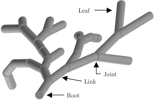
The previous sub-section introduced the concept of modeling a flexible instrument by enumerating all possible shapes and filtering the result according to given constraints. A natural way to implement this concept is to recursively create a spatial tree, whose growth is constrained by a set of filter functions. A spatial tree is an ordinary tree data structure, where each node represents a joint in 3D space. Each edge that connects a node with its child represents a link in 3D space. Each path from the root to a leaf represents a chain of links interconnected by joints and therewith is a discrete multibody representation of a flexible instrument. The entire spatial tree (all paths from the “root” to the “leaves”) represents the instrument's full workspace under the given constraints. A spatial tree can be created by a depth-first spanning tree algorithm, which recursively attaches links until it can proceed no more and then unwinds (backtracking) to a previous state where it picks a different link and again starts attaching links to it, and so on. Figure 5 shows a selection of paths of a filtered spatial tree.

Figure 5 Selected paths from the root to the leaves of a filtered spatial tree (FST).

A link is represented by a cylinder, which is attached to a coordinate system or reference frame. The reference frame is represented by a 4×4 matrix (homogeneous transform). In other words, the position and orientation of a link in 3D space is described by a matrix, denoted by F.

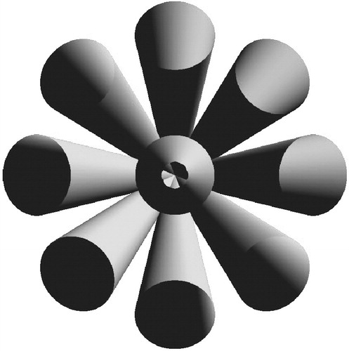
A joint is defined by the movements a link can make with respect to its predecessor. Starting from two aligned links (0° angle), parameter u describes the number of principal directions in which the second link can be moved. An example for u=4 could be “up”, “down”, “left” and “right”. Parameter v denotes the number of steps a link can be moved in each direction, and θ describes the rotation angle for each step. Figure 6 shows an example where u=8 and v=1. The number of possible positions between two adjacent links is uv+1, where the “+1” contributes for the “straight” (not moved) link, which is the default direction. The joint range is vθ.

Figure 6 A joint of the FST (frontal view), with u=8, v=1. Each cylinder represents a link in one of 9 (uv+1) joint positions. Note that the center link corresponds to a straight joint position, with a 0° angle between two adjacent links.

An algorithm f_gen() that creates a spatial tree takes a link F as input, attaches uv+1 links to F and recursively calls f_gen() for each attached link:where A is a link described by a matrix, T a translation matrix that moves F along its main axis towards its end, and R_i,j a rotation matrix that rotates F into the new position. The symbol ° denotes the concatenation of two links (matrices). Set {F T} contributes for the special case of two straight links, where a translation only is performed. The rotation matrix is given as an entry in a pre-computed look-up table of u columns and v rows:where R() is a rotation matrix which causes a rotation of jθ degrees about the ith rotation axis u_i.

For example, a set of 8 rotation axes can be found (u=8 and v=1) that produces a joint as shown in Figure 6. A perspective rendering of a frontal view of 9 link (uv+1) attached to a single link (occluded) is shown. The link in the center corresponds to an attached link which was translated but not rotated. Figure 7 shows an example for u=4 and v=3. The centerlines of all links (i=1 … u), which correspond to the same rotation angle jθ, lie on the surface of a cone. Different rotation angles j=1 … v correspond to different cones with concentric bases.

Figure 7 A joint of the FST, with u=4, v=3. Only the centerlines of the links, lying on the surface of concentric cones, are depicted. [Color version available online]

To prune the spatial tree as much as possible during creation, the filter function f_filter() is placed inside the recursion, so that, for example, colliding links get pruned immediately. If, for example, filter f_geometry() determines a collision with the organ wall, this branch is closed by not calling the recursion for the link. Similarly, a branch of the spatial tree is closed for filter f_energy() once the current energy is greater than the current energy minimum.

The look-up table for the rotation matrices is pre-computed, so that a rotation can be done with one 3×3 (only the rotation sub-matrix) matrix multiplication. This multiplication and the collision detection are the most expensive operations within the recursion.

Complexity of the FST algorithm

The time and space complexity of the FST algorithm is O((uv+1)ⁿ). However, depending on how much the growth of the spatial tree is constrained by the filter functions, the practical complexity, given a real anatomy, is more feasible. In particular, tubular structures, such as the tracheobronchial tree and vasculature, greatly limit the growth of the tree. The following experiment confirms this hypothesis:

Objective: To measure the empirical time and space complexity of the FST algorithm.

Method: Simulating the insertion of a catheter into a model of a brain artery using the FST algorithm. For the time complexity, the number of basic operations subject to the insertion depth is measured. Each recursive call is regarded as a basic operation. The space complexity is of the same order of magnitude as the time complexity, since each node of the spatial tree stores a constant amount of information.

Platform: PC, Pentium 4 dual, 1.3 GHz, 1 GB; Graphics: nVIDIA GeForce3, 64 MB.

Material: Model of a brain artery, reconstructed from planar parallel cross-sections (NUAGES [26], [27]), obtained from a patient-specific 3D rotational angiography (C-arm) scan. Number of triangles: approximately 25,000.

Design: For a fixed starting position, the flexible instrument model (u=8, v=1) was used to calculate a catheter of length n, inserted into the brain artery. This procedure was repeated 31 times for n=1, … , 31. For each calculation, the number of recursive calls needed to enumerate all possibilities, given the geometry and energy filter, was recorded.

Results: The result is shown in Figure 8. A fourth-order polynomial (y=1.1x⁴−39.4x³+426.3x²−1339.5x+538.7) can be fitted (least squares) to the resulting curve, indicating that the empirical complexity for this anatomy is O(n⁴). The second pair of curves shows the complexity after activation of two approximation methods described in the following section.

Figure 8 Empirical complexity of a catheter inserted into a brain artery. A fourth-order polynomial was fitted to the observed data from the FST algorithm. A linear fit was found for the data from the ∼FST algorithm. [Color version available online]

Observation: The first 17 links were computed in less than 1 second.

The approximated Filtered Spatial Tree (∼FST)

In the previous sub-section, a typical example was given demonstrating that the empirical complexity of the FST algorithm is polynomial (O(n⁴)) for tubular structures. In this sub-section, two approximative variants of the FST algorithm are presented, which together further reduce the empirical complexity to a linear bound. The new algorithm is called the approximated Filtered Spatial Tree (∼FST).

The ∼FST algorithm incorporates two approximation schemes: the (n′, k)-approximation and the (u, v)-approximation. The first follows the idea of composing an instrument of length n from several “sub-instruments” of length n′≪n. The second constrains for each execution of the FST algorithm the maneuverability of each joint to only one possible angle. For a detailed description of both approximation schemes see [24], section 1.3.2.

An experiment similar to the previous one was conducted to determine the empirical complexity of the ∼FST algorithm. The result is shown in Figure 8. A linear function (y=761.4x+4358) can be fitted (least squares) to the resulting curve, indicating that the empirical complexity for this anatomy is O(n).

Model-based guidance of TBNA without a computer in the operating room

In performing a TBNA the surgeon faces two major problems: First, hitting the target requires 3D imagination (coordination of the learned 3D anatomy with a fish-eye distorted 2D video image) together with the handling of the endoscope (hand-eye coordination). Secondly, assessing how many tissue samples to take is a trade-off decision between patient safety and probability of success.

This section presents a new guidance method for TBNA biopsies that helps the bronchoscopist with both problems. The basic idea is to calculate a TBNA protocol. Regarding the first problem, the protocol describes in detail how to perform a series of tissue samplings, by prescribing for each sample how to handle the bronchoscope in order to move the biopsy needle into the target lesion. Regarding the second problem, the protocol gives the probabilities of success for each tissue sample. This allows the bronchoscopist to decide whether or not the gain of an additional biopsy justifies the associated discomfort and risk for the patient. During the operation, the bronchoscopist executes the protocol by setting the bronchoscope to the prescribed configuration. To gain control over the current configuration of the bronchoscope, a set of passive controls is used to monitor its degrees of freedom.

The endoscope model previously described in the section headed A real-time deformable model for flexible instruments is used to preoperatively simulate the insertion of a bronchoscope into a target branch of the tracheobronchial tree. The result is a set of candidate shapes for the unknown shape of the bronchoscope during the intervention. This set represents the initial position domain for the “optimal” k-needle placement strategy as introduced earlier.

The foundation of this TBNA guidance technique is an accurate model of a flexible endoscope, including its actively bendable tip. Accordingly, the approach described here is denoted as a “model-based” approach.

Related work

Techniques in the literature for guiding TBNA can be classified into three different groups: imaging-based, vision-based and sensor-based approaches.

Imaging-based approaches use standard imaging techniques like conventional fluoroscopy, CT-fluoroscopy, computed tomography (CT), and ultrasonography to visualize the endoscope, the advancing needle, and the target lesion.

Conventional fluoroscopy (C-arm imaging) produces a 2D projection image (X-ray) in real time with limited inferior contrast resolution. The target lesion is usually not identifiable as a distinct structure [28], due to the superimposition of structures in the mediastinum. To keep the needle in the image plane, the position of the C-arm must be updated frequently.

CT-fluoroscopy is a term for continuous-imaging CT that allows the visualization in real time (currently up to 64 slices) of dynamic processes such as the insertion of a needle into the target lesion. White et al. [28] reported a clinical study in which TBNA was successfully performed under CT-fluoroscopy guidance. In a later study [29], the same group reported that CT-fluoroscopy provides effective, real-time guidance for TBNA, and may be particularly valuable in patients with small or less accessible mediastinal lung lesions.

Conventional CT produces images of adequate resolution, but the procedure is cumbersome and time-consuming since real-time imaging is not possible and each sequence must be prescribed in advance.

Ultrasonography was used by Shannon et al. [12] to visualize the target lesion by inserting a catheter-enclosed ultrasound transducer through the working channel of the bronchoscope. A motor in the ultrasound unit rotated the transducer within the catheter, producing a cross-sectional ultrasound image oriented perpendicular to the long axis of the catheter. However, this study showed no significant difference in sensitivity when compared to unguided TBNA. Images obtained from the sonography probe are of variable quality, user-dependent (probe pressure) and may not be diagnostic. Furthermore, the transducer and needle share the same port and cannot be inserted simultaneously, so real-time imaging during needle insertion is not possible. In a recent study, Herth et al. [30] reported that endobronchial ultrasonography (EBUS) is simply performed and, if used for TBNA guidance, affords an excellent yield independent of lymph node location. A new convex probe, CP-EBUS, with the ability to perform real-time TBNA under direct ultrasound guidance, has been developed by Yasufuku et al. [31] in collaboration with Olympus Corporation (Tokyo, Japan). First preliminary results indicate that CP-EBUS has excellent potential for assisting in safe and accurate diagnostic interventional bronchoscopy.

Vision-based approaches use only the image information from the bronchoscope's optical system (fiber-optics or CCD chip) to track the instrument tip. This is an elegant approach since it generally requires no additional devices. The idea was pioneered by Bricault et al. [32–34], who were able to compute the position and orientation of the tip in a special situation where a bifurcation was shown in the image. The tracking would fail if no bifurcation were shown.

Sherbondy et al. [35] proposed a two-step approach that requires the cooperation of the bronchoscopist. In step one (preoperative), the user interacts with the 3D CT data by means of a virtual endoscopy environment and selects a “key-site” from which he wishes to perform the biopsy. A virtual view from this site is recorded. During stage two (intraoperative), the bronchoscopist moves the real endoscope as close as possible to the “key-site”. The virtual view is then registered to the current real view, using an iterative mutual-information-based matching. All presented results are based on key-sites showing a bifurcation.

Mori et al. [36] reported having achieved continuous tracking of the bronchoscope tip, even in the absence of strong features such as a branching structure. These authors used epipolar geometry analysis and an image-based registration technique. The main idea is to match real endoscopic views with virtual endoscopic views. However, the computation time is 20 seconds per frame, which is not feasible for real-time procedures.

Sensor-based approaches use external sensors attached to the bronchoscope to determine the tip position and orientation. A new technology called ShapeTape (Measurand, Inc., Fredericton, New Brunswick, Canada: www.measurand.com) might be used to visualize the entire endoscope within the tracheobronchial tree. ShapeTape is a lightweight, flexible ribbon with an array of fiber-optic sensors along its length that measures its bend and twist. Attaching the ribbon to a flexible endoscope could allow the endoscope's shape to be measured in 3D. This technology has not yet been applied to guiding flexible endoscopic procedures.

The Biosense intrabody navigation system (Biosense, Setauket, NY) uses electromagnetic fields to track a 1.5-mm sensor that can be attached to the bronchoscope tip. Solomon et al. used this system in an animal study (in swine) [9] to determine the feasibility of using real-time tracking technology coupled with preoperative CT data to enhance TBNA. Prior to CT scanning, 10–20 metallic nipple markers were secured on the animal's anterior chest wall and their coordinates were later identified in the CT dataset. To register the sensor's position with the CT images, the sensor, while attached to the bronchoscope tip, was touched to the nipples. Another registration problem was caused by respiratory motion during the intervention, which causes deformations not included in the static preoperative CT dataset. Continuously drawing the sensor's position in the static CT dataset will sometimes show the tip of the bronchoscope to be in physically impossible positions, e.g., outside the airways. According to the authors, this situation was assessed by the bronchoscopist to be “confusing”…

To compensate for this difficulty, a second position sensor was attached to the animal's chest wall to gate respiratory motion. The position of the bronchoscope tip was updated on the CT image monitor when the animal was in a stage of the breathing cycle that corresponded to the breathing state during image acquisition. The study showed an in vivo accuracy of 4.2 mm±2.6 mm (standard deviation). Using the same system, Solomon et al. later reported [37] an accuracy of 5.6 mm±2.7 mm in a study with 15 adult patients. The authors also investigated the feasibility of a new registration method that involves touching internal structures of the tracheobronchial tree instead of external skin markers (metallic nipples). This new method was subjectively judged to be superior for registering the position of the bronchoscope, but its exact accuracy was not determined.

A model-based approach to TBNA guidance

The motivation for developing a new approach to TBNA guidance comes from the shortcomings of existing approaches.

Imaging-based approaches like fluoroscopy, CT-fluoroscopy and CT imaging require significant and expensive scanner time and cause additional radiation exposure for patients and staff. Although sonographic guidance of TBNA may ultimately prove useful, the technique proposed by Shannon et al. suffers from two limitations. First, the diagnostic quality of the images obtained with the sonographic probe is variable and therefore highly operator-dependent. Second, the bronchoscopic port that is used for the ultrasound probe is the same as that through which the biopsy needle is passed. However, these limitations may be overcome by the newly developed special-purpose CP-EBUS bronchoscope proposed by Yasufuku et al. [31].

Vision-based approaches cannot be considered as a mature technology since tracking is either unreliable or incapable of real-time processing. The approaches by Bricault et al. [32–34] and Sherbondy et al. [35] rely on the existence of strong features in the images, which is not always the case. The approach of Mori et al. [36] showed satisfactory tracking results, but with a processing time of 20 seconds/frame, the approach is far from ready for real-time clinical application. Considering a peak acceleration of the bronchoscope during the intervention and an additional simultaneous acceleration caused by active bending of the tip, it can be assumed that a processing time of about 30 fps is necessary to assure reliable tracking. To achieve this frame rate, the algorithm proposed by Mori et al. would require a speed-up by a factor of 600.

Sensor-based approaches seem to be the most obvious way to guide TBNA biopsies. However, a general problem is the increase in size of the bronchoscope caused by fixing sensors to the outside of its tip or shaft. Furthermore, cables have to be passed all the way along the outside of the shaft to the sensors. This represents a major problem for sterilization. A potential solution to the latter problem is to design a new type of bronchoscope that contains the sensor and cables inside it. However, this would require hospitals to buy new and probably expensive equipment. Another concern is that this approach would counteract the current promising trend towards developing ultra-thin bronchoscopes capable of reaching down several levels of bifurcations.

Registration between the sensor coordinate frame and the CT dataset represents a further difficulty. Solomon et al. [37] use a large number of metallic nipples that need to be affixed to the patient's chest prior to the scan. This leads to two problems: First, the time between the scan and the TBNA should be kept to a minimum, since the longer the interval the greater the chances that the patient will change or the nipples will move or even fall off. Second, the patient has to be scanned twice. The first scan leads to a diagnosis and the need for the patient to undergo a TBNA, but the patient must then be scanned again with the metallic markers in place.

Calculating a TBNA protocol

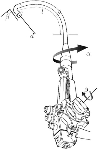
The approach described here for guiding TBNA biopsies is based on the idea of preoperatively calculating a TBNA protocol. The term “protocol” is used in the sense of a detailed plan (step-by-step instructions) for a medical procedure. The protocol prescribes how to handle the bronchoscope to achieve a successful biopsy. Describing the handling of a bronchoscope requires parameterization of all its degrees of freedom. Figure 9 shows an endoscope and its degrees of freedom with reference to an insertion into a tubular structure like the tracheobronchial tree. Given that the bronchoscope resides “somewhere” inside a predetermined target branch, the following four parameters well define a TBNA-biopsy:

1. Bronchoscope insertion depth l.

2. Shaft rotation about the principal axis α.

3. Angle of tip deflection β controlled by the bronchoscope's angling wheel.

4. Needle length d.

These parameters are denoted as an endoscope configuration c=(l, α, β, d). Parameters α, β, d are also called alignment parameters. An endoscope configuration c is called a “successful configuration” if the needle tip of an endoscope set to c is located inside the target lesion.

Figure 9 The handling of an endoscope can be parameterized using four parameters: l, α, β and d.

During the operation, the bronchoscopist executes the protocol by setting the bronchoscope to the prescribed configurations. To ensure control over the current configuration of the bronchoscope, a set of passive controls is used to monitor parameters l, α, β and d (see section headed Controlling the protocol execution below).

The goal now is to calculate, for a given biopsy scenario, a minimal set of endoscope configurations of which one is a successful configuration. To allow the bronchoscopist to assess how many tissue samples to acquire, the probability of success for each sample is also required. The following lists the necessary steps involved in calculating a TBNA protocol, which includes both pieces of information:

1. Reconstruct from planar parallel cross-sections a 3D model of the tracheobronchial tree and the target mass.

2. The radiologist/bronchoscopist preoperatively plans biopsy site b.

3. Calculate the bronchoscope length l needed to reach b.

4. Calculate the bronchoscope's workspace W (see above), given its length l and the branch containing b as the branch of interest.

5. Calculate a needle placement strategy (see above), given workspace W (candidate shapes) as the initial position domain P.

The basic idea behind the algorithm is to regard the procedure of performing a TBNA biopsy as a two-step process: First, the bronchoscope is inserted into the target branch, after which the instrument's insertion depth is kept fixed. Secondly, the bronchoscope tip is aligned (fine tuning) with the target lesion and the needle is advanced into the tumor. This allows calculation of the endoscope parameters α, β, d based on a fixed insertion depth l.

In step three the endoscope model described previously is used to calculate the insertion depth l needed to reach biopsy site b. The length is calculated with respect to reference point r. In a later referencing step (see next sub-section below), r is related to the actual position of the passive length control outside the body. Based on insertion depth l, the algorithm ∼FST calculates the bronchoscope's workspace in step four. The workspace is a set of bronchoscope shapes, representing possible candidate shapes for the real bronchoscope, inserted into the same branch. Since all shapes of the workspace are of length l, the alignment parameters α, β, d can be calculated in step five, using the kCP_Greedy()'' algorithm shown in Figure 25.

Registering the virtual with the real bronchoscope

This section deals with the issue of registering the bronchoscope parameters l, α, β, d, derived from a preoperative 3D dataset, with the current configuration of the bronchoscope during the intervention. For each parameter a mutual zero point regarding preoperative planning and the patient's reference frame has to be found. For parameter β the straight tip (0° bending) and for d the needle length just before leaving the working channel (0 mm infeed) can be used. For parameters l and α a landmark-based approach has been used. The main carina, a keel-shaped part of the tracheobronchial tree which marks the bifurcation of the trachea into the left and right lungs, can serve as a mutual zero-point for both parameters.

Regarding the insertion depth, the idea is to touch the carina during the intervention with the bronchoscope. This state can be recorded as the zero position for the insertion depth by marking off the endoscope length, e.g., at the patient's mouthpiece. The corresponding protocol parameter l has to be calculated relative to this length. The situation is shown in Figure 10. Let denote the length of the bronchoscope from the mouthpiece to the landmark (carina). The insertion depth l, needed for the biopsy, can then be given as an offset to . This offset can be calculated as the difference between and .

Figure 10 Landmark-based registration. The insertion depth to the biopsy site can be given as an offset to the insertion depth to the main carina.

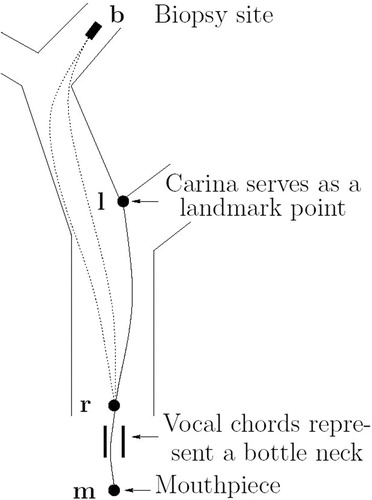
Reference point r was chosen to lie right behind the vocal chords, because these represent a bottleneck for all possible paths a bronchoscope can take. This justifies the use of the createFST() algorithm for length calculations, since this algorithm requires a fixed start link.

Regarding the shaft rotation, the rotation angle, which, for example, shows the carina to appear vertically, can serve as a zero point. During the intervention, after touching the carina, the bronchoscopist withdraws the bronchoscope until the carina is fully visible. Then he rotates the shaft until the carina appears vertically. This angle can be recorded as the zero position by a mark on the control outside the patient. During the planning phase the same angle can be determined by rendering a view from a virtual endoscopic camera. The radiologist/bronchoscopist rotates this virtual view until it shows the main carina appearing vertically. The shaft rotation α, needed for the biopsy, is then given as an offset to this angle.

The proposed landmark-based registration technique is less sensitive to respiratory motion than, for example, a technique based on a set of external markers. External markers that are attached to the patient's chest move considerably during the respiratory cycle. There is thus a problem in relating these moving markers to the corresponding markers in the static CT data set of the patient. In contrast, the carina is in close proximity to the center of the body and is therefore expected to move less than a marker located on the patient's chest. More importantly, however, it can be assumed that landmark and target move in sync during respiration. In other words, there is only a little movement of the target relative to the carina, and this may also result in good accuracy in a breathing patient.

Controlling the protocol execution

To set the bronchoscope to the configuration given by the protocol parameters, control over the inserted length l, the shaft rotation α, the tip deflection β and needle length d is required during the intervention. Figure 11 shows a set of passive (non-electronic) controls for controlling all parameters.

Figure 11 Passive controls for monitoring the endoscope configuration.

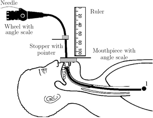
Since the biopsy is performed on the basis of a fixed bronchoscope length, a stopper is used to prevent the bronchoscope from penetrating the body more deeply than desired. To set the insertion depth of the bronchoscope, the stopper is moved l mm away from the base-plate of the mouthpiece (as measured using a ruler), while the bronchoscope is in the zero position, which means touching landmark l. The stopper is locked at this position using a rubber ring. Note that the use of a mouthpiece (bite guard) is highly recommended [38] to avoid damage to the bronchoscope by the patient's teeth. To control the shaft rotation, a pointer has been attached to the stopper and a goniometer (angle-scale) has been attached to the base-plate of the mouthpiece. When the bronchoscope is in the zero position with respect to the shaft rotation, i.e., when the bronchoscopic image shows the main carina appearing vertically, the pointer is moved to a zero mark on the goniometer. When the base-plate stops the insertion of the bronchoscope (due to the locked stopper), any shaft rotation moves the pointer along the angle-scale, indicating the current offset to the (vertical) main carina. To set the shaft rotation, the bronchoscope is rotated α degrees relative to the zero mark.

Tip bending is controlled by an angle-scale attached to the angling wheel located at the bronchoscope's control head. During the planning phase, a look-up table is computed that maps the angle of tip deflection to the wheel angle. The needle length is controlled by marks on its proximal end and by using the opening of the biopsy port as the zero point.

The generic TBNA protocol is shown in Figure 12.

Figure 12 The TBNA protocol, including patient-non-specific instructions and patient-specific parameters (l, α_i, β_i, d_i).

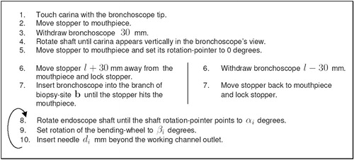
Experiments and results

This section presents experiments and results for the previously described endoscope model, TBNA protocol and needle placement strategy. Additional experiments and more detailed analysis can be found in [24].

Validation: endoscope model

This section presents experiments conducted to validate the flexible instrument model described in the previous sections. A general approach to validating a mathematical model of a real-world object is to measure the object with respect to some world coordinate system, transform the measures into the model coordinate system, and subsequently compare both representations. If the real-world object interacts with its environment, a mathematical model of this environment is needed as well.

The biggest difficulty in this scenario is measuring the real-world object without using procedures that influence or alter the object's shape. The object should be acquired in its natural behavior, uninfluenced by external measuring devices. For this purpose, a new type of passive, retro-reflective marker was used which works with standard, off-the shelf optical tracking systems. By using cylindrical markers, it is hoped that the tracking system's built-in software will be able to accurately determine the center of the cylinder's rectangular projections and correctly triangulate the cylinder's center. The idea is to wrap a strip of retro-reflective material around the shaft of the endoscope, such that its projection is “square-like”. Figure 13 shows a photograph (taken with flash illumination) of an endoscope with 30 cylindrical markers.

Figure 13 Experimental setup. Olympus GIF-100 with retro-reflective markers inserted into an “M”-shaped calibration path. The endoscope's shape (centerline) was measured in 3D space, using an optical stereo tracking system.

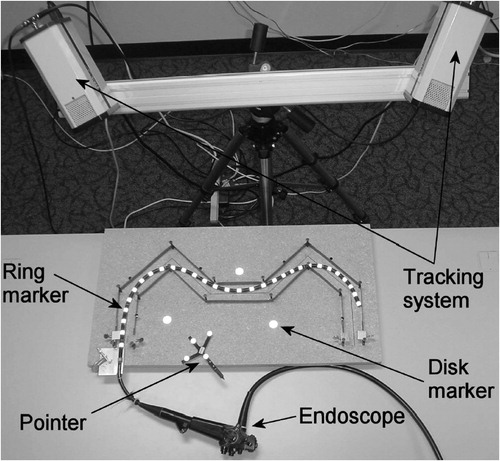
Since the accuracy of regular off-the-shelf tracking systems is specified only for ball- or disk-shaped markers, an experiment was performed to determine their accuracy with respect to cylindrical markers. The results show that the tracking system used was able to accurately measure the centerline of a real endoscope in 3D space. Details regarding the design of the experiment and the results can be found in [24], chapter 1.5.1.

Calibration phantom and lung phantom

This section presents an experiment to quantitatively assess the accuracy of the model and several figures to visually demonstrate its usefulness. The experiment is based on a calibration phantom, while the figures show the model inside a lung phantom derived from a CT scan of the model shown in Figure 19.

In the experiment, the method for accurately determining the centerline of an endoscope in 3D space is used for model validation. The idea is to insert the real endoscope into a calibration phantom and measure its shape. The digital endoscope model is then inserted into a digital model of the calibration phantom. By transforming the measured endoscope shape from the coordinate system of the tracking system into the coordinate system of the digital models, both shapes can be compared with each other. The experimental setup is shown in Figure 13. The “M”-shaped calibration phantom (length: 1050 mm; width: 50 mm) was designed to be open, to allow a direct line of sight for the tracking cameras, and to be simple enough that a digital model could be easily obtained.

The result is shown in Figures 14 and 15. Figure 14 presents an example with n=16 and k=2. It shows as an intermediate result the first 13 segments, which means that 26 links out of n=44 have been computed. For Figure 15, n′=20 and k=4. To take account of the frictional forces acting on the endoscope tip, p=7 [Equation 15] was set for the last segment and p=1 was set for all others. The figure shows the best match between the markers (black balls) and the model. The model consists of 9 segments (color coded), the first 8 each consisting of 4 links, the last of 12 links. Each link was 20.45 mm long. For the last segment, the 7 smallest energies were computed and displayed. One of these matched the last 6 markers by a (modified) Hausdorff distance of 0.8 mm. More details regarding the design of the experiment and the results can be found in [24], section 1.5.2.

Figure 14 Endoscope model inserted into the calibration path model. Intermediate results (n=44, n′=16, k=2) after the first 13 segments were calculated. All “tentacles” are shown full length. [Color version available online]

Figure 15 Final result (n=44, n′=20, k=4, p=7), showing only the first k=4 links of each tentacle. For the last segment the energy constraint has been relaxed by computing the p=7 smallest energies. The endoscope model largely matches the measured markers of the real endoscope. [Color version available online]

In this experiment, no explicit assumptions were made about the endoscope lying on a planar surface. Only the start link was placed to lie on the bottom of the 3D “M”-path model. The torsion term E_τ() of the deformation energy function [see Equation 15] prevented the model from moving out of this plane. An experiment described in the next sub-section below showed similar results for an endoscope inserted into a 3D lung phantom.

Figures 16 and 17 show the results of two insertion simulations into a lung phantom. The figures demonstrate the model's realistic behavior and robustness by producing animations that show the instrument smoothly sliding down different anatomies. The rigid sleeves of the endoscope's bending section are displayed in red and green, while the flexible part is displayed in yellow. Starting with an initial insertion depth, a model of the respective instrument was calculated and the result displayed. Next, the insertion depth was increased by a fixed step size and another model was calculated and displayed, and so on. In other words, no information from the model at insertion depth x mm was used to compute the new model at insertion depth x+1 mm, given a 1 mm step size. For the second animation (active bending), a total of 60 instruments (2 mm step size) were computed in 60 s. The flexible part of the bending section (yellow) was configured to have a maximum range of 90°. The result shown in the last image corresponds precisely to the maximum achievable insertion depth of the real bronchoscope (GIF-100) inserted into the same branch of the lung phantom.

Figure 16 Insertion simulation at 12 different stages: After insertion to a depth of 420 mm, the endoscope became stuck due to insufficient branch diameter. [Color version available online]

Figure 17 Active bending simulation: How far can the Olympus GIF-100 reach into the upper right lobe of the lung phantom? [Color version available online]

For the first animation, a total of 240 instruments (1 mm step size) were computed in 27 s. The significant time difference is due to the fact that the first animation required a higher flexibility for the bending section. Therefore, the ranges of the corresponding joints were much higher than for shaft joints. Consequently, v (the number of rotation steps per joint) is higher for the first animation, which significantly increases its run-time. More details regarding the animations and their timing can be found in [24], section 1.6.

Although appropriate for determining the algorithm's average run-time for single instruments, the above-described implementation is inefficient for calculating continuous insertion simulations. For such a task, only one spatial tree should be built in a single call to the ∼FST algorithm, since all information accumulated for insertion step i can be used to calculate step i+1. In other words, if all information at step i were used in the computation at step i+1, the overall run-time for n steps would be similar to the run-time needed for the last step n alone. A tree of depth n includes all leaves of a tree of depth n−1, which includes all leaves of a tree of depth n−2, and so on. For the first animation 4 s were needed to calculate the last (longest) instrument, whereas for the second animation less than one second was needed.

Figure 18 demonstrates how endoscopes of varying degrees of deformation can be generated by stepwise tightening the selectivity of the energy filter. From top left to bottom right, paramter p in Equation 15 was decreased from p=∞ to p=1.

Figure 18 The deformation energy decreases from top left to bottom right. [Color version available online]

Validation: TBNA protocol

This section presents two experiments to investigate the feasibility of guiding TBNA biopsies by executing a TBNA protocol (model-based approach).

Repeatability

The objective of this experiment was to investigate the feasibility of guiding TBNA biopsies by executing a TBNA protocol. The first questions that needed to be answered were: (1) Could the endoscope's insertion depth, shaft rotation, bending angle and needle length be reliably controlled, using the passive controls described earlier, and (2) how accurate was the proposed landmark-based registration method, or, in other words, how reliably could the endoscope be set repeatedly to the respective zero position for insertion depth and shaft rotation?

The experiment was designed to measure the repeatability of hitting a target point visible on the inner wall of the lung phantom. In the first step, the registration procedure of the TBNA protocol was executed. In the second step, the endoscope was moved into the target branch of the lung phantom. The third step was to use the CCD camera in the endoscope tip to touch the target point with the biopsy needle. In the fourth step, the current shaft rotation, bending angle and needle length were read from the controls and recorded. Steps 1–4 were repeated 20 times for the same target. Based on these measures, the variation of parameter α, β and d, given a fixed insertion depth l, were calculated. This test was performed five times, each time for a different target point.

The results show that the average and worst range (i.e., the difference between the smallest and largest values) for α, β and d were 6°, 4°, and 4 mm, and 7°, 6°, and 7 mm, respectively.

Endoscope model accuracy

The objective of this experiment was to investigate the following question: How accurately could the shape of the Olympus GIF-100, inserted into the lung phantom, be predicted in a pre-operative simulation, using the endoscope model described earlier?

The experiment was designed to use the optical tracking system for measuring the shape of the Olympus GIF-100 inside the lung phantom. Figures 19, 20 and 21 show the experimental setup, consisting of the tracking system, the lung phantom and the endoscope with the cylindrical retro-reflective markers. The measured shape was then compared to the shapes generated by the endoscope model.

Figure 19 Experimental setup, showing the lung and head phantom and the endoscope with the biopsy needle.

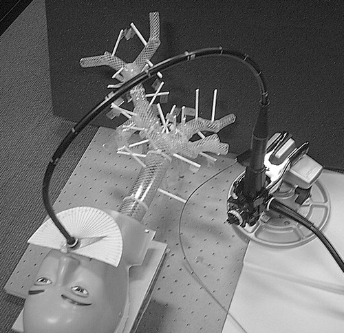
Figure 20 Experimental setup showing the tracking cameras and lung phantom.

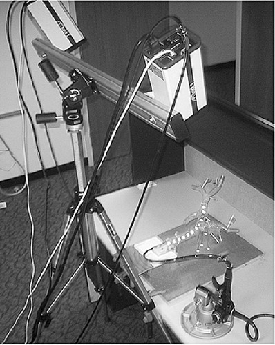
Figure 21 Experimental setup showing the Olympus GIF-100 with reflective markers inserted into the lung phantom.

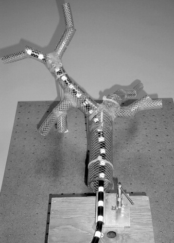
The endoscope was maneuvered to five different sites within the lung phantom. At each site, the positions of the markers detected by the tracking system were recorded. Also, the insertion depth was recorded for each site.

The virtual endoscope was then maneuvered to the same sites, with the same insertion depth, using the create ∼FST() algorithm. For each site, 10 endoscope shapes were calculated by setting the selectivity of the energy filter to p=10. For each site, the measured shape, given by the coordinates of the cylindrical markers, was compared to the 10 virtual endoscopes.

To compare the measured endoscope with the virtual endoscope, a coordinate transformation had to be found that mapped the coordinate system of the tracking system into the coordinate system of the endoscope model. To solve this registration problem, a method according to the ICP (Iterative Closest Point) algorithm [39] was used. At first, a set of corresponding reference points is specified in both datasets. Subsequently, a rigid body transformation is calculated that represents the best fit in the least-squares sense between the two sets of reference points. To solve the resulting non-linear minimization problem, the Levenberg-Marquardt method [40] is used.

The result is shown in Figures 22 and 23. Figure 22 shows one of the five measured shapes of the Olympus GIF-100 and Figure 23 shows the corresponding virtual endoscope, generated by the create ∼FST() algorithm. In Figure 22, two adjacent marker positions are connected by a cylinder. The figures show that the measured shape of the endoscope matches closely the shape of the virtual endoscope, especially at the tip. For a detailed quantitative analysis see [24], experiment 3.7.

Figure 22 Model accuracy: measured shape. [Color version available online]

Figure 23 Model accuracy: predicted shape. [Color version available online]

Validation: needle placement strategy

The following section describes an approximative algorithm, which at each stage greedily constructs a solution by selecting the sub-solution that gives maximum improvement. The subsequent section describes an experiment to validate the approach by simulating a TBNA using the endoscope model described earlier. The algorithm described below was implemented to calculate a list of needle parameters and probabilities for a given number of needles. The resulting list shows that the approach can provide valuable decision support for the physician in choosing how many needles to place and how to place them.

kCP_Greedy() algorithm

This section describes an algorithm called kCP_Greedy(), which represents a greedily constructed solution to the Maximum k-Coverage Problem. The algorithm is described on the basis of a concrete application, namely a TBNA.

The idea is to use the endoscope model described earlier to simulate a TBNA by calculating a set of possible endoscope shapes (workspace), given a target branch and insertion depth. This set of candidate shapes represents the initial position domain P^Δ. For each shape in P^Δ an artificial target T^Δ⊂IR³, modeled as an elliptic point cloud, is scanned (S^TΔ(p)). An example of such a scenario is shown in Figure 24.

Figure 24 Endoscope model (workspace) inserted into a lung model. Target T is represented by an elliptical point cloud. [Color version available online]

For each point t of the target point cloud, three endoscopic parameters are determined which move the tip of the biopsy needle into position t: shaft rotation α, angle of tip deflection β, and needle length d [see Equation 1]. These parameters represent a point in the needle parameter domain N^Δ⊂IR³. A complete scan of T^Δ from one viewpoint results in a point cloud in N^Δ. A complete scan from all viewpoints results in a set of point clouds in N^Δ. This set of point clouds (see Figure 4) represents the input to the kCP_Greedy() algorithm.

The set of point clouds is given bywhere x, y, z∈IR^l and p∈IN^l are l-dimensional column vectors:

Let x_i denote the i^th element of vector x so that (x_i, y_i, z_i, p_i) represents the i^th “row” of I, for i=1,…, l. The first three parameters of a row represent the x-, y- and z-coordinates of a point in the needle parameter domain N. The fourth parameter p_i represents the number of the corresponding viewpoint. As in Figure 4, the viewpoints are numbered 1 to |P^Δ|, so p_i∈{1, 2, …, |P^Δ|}.

The algorithm given in Figure 25 describes the kCP_Greedy() approach in pseudo-code. The description follows the basic structure of a Matlab (The MathWorks, Inc., Natick, MA) implementation. The full Matlab code of this implementation can be found in Appendix A of [24].

Figure 25 The algorithm kCP_Greedy().

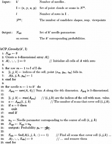
Array A() (line 2) can be regarded as a set of 3D arrays, each of which corresponds to a scan from one of the viewpoints in P^Δ. In other words, the size of A() along the fourth dimension is |P^Δ|. The size along the first three dimensions (x-, y- and z-coordinates of a needle parameter) is given by the difference between the maximum and minimum parameter values, divided by the desired cell size Δ_N. The instruction in line 11 corresponds to a projection of A() from 4D to 3D. All 3D (needle parameter) arrays are merged (summed) together to one 3D array. S_idx in line 23 is a set of subscripts. Each subscript denotes a 3D array (scan) that has a “1” at position (i, j, k).

An “optimal” TBNA biopsy strategy

This section describes an experiment for testing the kCP-approach to the problem of finding an optimal biopsy strategy for a TBNA. The scenario is shown in Figure 24. The model described earlier was used to calculate a set of candidate shapes for the endoscope. An optimal set of needle parameters that covered these candidate shapes and the corresponding probabilities were computed using the kCP_Greedy() algorithm in Figure 25. The result is a table that could give valuable decision support to the bronchoscopist in choosing how many biopsies to perform and how to perform them.

Objective:

1. Visualization: The first objective was to validate the approach by visualizing a scan of target T^Δ in the needle parameter domain N^Δ. Based on this visualization, several scans from different viewpoints were rendered to assess the amount of overlap.

2. Biopsy strategy: The objective here was to calculate needle parameters n_i∈N^Δ for i=1, 2, …, k needles and the corresponding probabilities.

Method: The set of initial positions P^Δ was given by the first rigid sleeve (red link in Figure 24) of the bending section of all endoscope shapes in the workspace (|P^Δ|=283). Function f_free: P^Δ×T^Δ→N^Δ represents a model for the endoscope's bending section without any restrictions in its movement. In other words, all t∈T^Δ can be reached by the needle. As described by Equation 1, for a given link and target t, f_free calculates the following three parameters needed to bring the biopsy needle into position t: shaft rotation α, bending angle β and needle length d. These three parameters form the needle parameter domain N^Δ⊂IR³.

The unrealistic assumption of unrestricted tip movement was omitted with function f_coll. This model uses collision detection to determine whether or not the tip of the endoscope can be bent to reach a target t.

Platform: SGI 540 PC, Pentium 3 single, 550 MHz, 500 MB; Graphics board: Cobalt Graphics, 48 MB.

 Material:

1. Patient scan (CT) of the tracheobronchial tree (Figure 24).

2. Deformable model of a flexible endoscope as described previously.

3. Functions f_free: P^Δ×T^Δ→N^Δ and f_coll: P^Δ×T^Δ→N^Δ, which represent a model for the endoscope's actively bendable tip.

4. The target of a TBNA is an enlarged lymph node, which is of circular or elongated shape and is typically about 10 mm long. Such a lymph node was modeled as an ellipsoid of 10 mm length and 4 mm width. The ellipsoid was represented and rendered as a point cloud T^Δ consisting of 5,000 points.

5. Visualization of the scans was done using Matlab.

6. A Matlab implementation of the kCP_Greedy()algorithm.

Results

(1) Visualization: Figure 26 shows 10 scans, each represented as a lit convex hull of the original point cloud. Each point in the point cloud represents a value for shaft rotation, bending angle and needle length. Figure 27 shows the same scenario, with each scan rendered with a 0.5 transparency value (alpha blending). Note the considerable overlap of these randomly chosen scans in 3D.

Figure 26 Ten scans of T^Δ, rendered as lit convex hulls of the respective point clouds. [Color version available online]

Figure 27 Same scans as in Figure 26, but each rendered with a 0.5 transparency value (alpha blending). Bending model: f_free. [Color version available online]

Figures 28 and 29 correspond to Figures 26 and 27, with the difference that now the bending model f_coll was used. The movement restriction of the tip, caused by the physical confines, does not allow for a “full” scan of the target from a given initial position. Consequently, only portions of the scans in the previous figure remain. However, the overlap between the scans is still considerable.

Figure 28 Same scans as in Figure 26, but using bending model f_coll. [Color version available online]

Figure 29 Same scans as in Figure 27, but using bending model f_coll. [Color version available online]

(2) Biopsy strategy: Figure 30 shows a series of screen shots from the Matlab implementation of the kCP_Greedy() algorithm, using bending model f_coll. Figures 30a to 30l depict the needle parameter domain N^Δ. The grid indicates the cells in N^Δ. The cell size is given by 5°×5°×2 mm. Each scan of target T^Δ is depicted as a transparent (alpha blending), unlit (flat shading) convex hull. Figure 30a shows the scans from all viewpoints in P. In Figure 30b the cell of maximum coverage was determined, all scans covering this cell were removed, and a “1” was drawn in the center of that cell. Given the remaining scans, the cell of maximum coverage was determined, all scans covering this cell were removed and a “2” was drawn in the center of that cell. The result is shown in Figure 30c. This procedure was repeated until 99.9% of the scans were removed (Figure 30l). Each number i drawn in N^Δ represents an alignment parameter α_i, β_i, d_i. Computation time was approximately 2 min.

Figure 30 Screen shots from the kCP_Greedy() Matlab simulation. Figures (b)–(g) correspond to needles 1–6 in Table I. [Color version available online]

The percentage of scans removed in each step corresponds to the probability of success for the respective biopsy needle placement. This probability and the cumulative probability was calculated for needle i=1 … 6 as |V_i|/(|P^Δ|=283). The result is shown in Figures 30b–30g and in Table I.

Table I.  Probability of success for each needle placed.

Needle	1	2	3	4	5	6
Probability [%]	42	28	16	4	4	3
Sum	42	71	86	90	94	97

The table shows that two needles cover 71% and three needles 86% of all initial positions, and represents a valuable decision support tool for the bronchoscopist. Depending on the concrete condition of the patient, he/she can decide whether or not a third or even a fourth needle is advisable. Based on this table, a third needle gives a considerable improvement of 16%, whereas the improvement offered by a fourth, fifth or sixth needle is negligible (≤4%).

Conclusion

We have presented an “optimal” strategy for placing k biopsy needles given a large number of possible initial needle positions. This problem arises, for example, in guided, endoscopic needle biopsies, where the position of the endoscope tip is known with some degree of error. Beside the actual needle parameters, a table is provided for the physician that contains the probability of success for each needle. By placing the needles in order of decreasing probability, the physician can decide after placing each needle whether the gain in overall probability of success obtained by employing the next needle outweighs the risk to the patient. Overall, the approach can provide valuable decision support to the physician regarding how many needles to place and how to place them.

This general concept has been applied to the clinical problem of guiding transbronchial needle aspiration biopsies. To obtain an estimation of the bronchoscope's position before needle placement, a new model for flexible instruments has been developed. The model can be configured to represent either catheters or endoscopes. Special attention has been paid to modeling certain mechanical constraints often found with flexible endoscopes: a tip that can be bent to a much higher degree than the general shaft flexibility, rigid sections (sleeves) within the bendable tip, a considerable shaft diameter, and a slightly bigger tip diameter.

An interesting property of the model is the option of generating several similar shapes for the instrument tip. The model requires no initialization in the form of an initial “good guess” (spline control points) of the final shape, and no preprocessing. Furthermore, a method for measuring the centerline of a real endoscope has been developed. This method uses a new type of marker that does not significantly alter the shape of the endoscope and therefore does not influence the outcome of the measurements. It has been used to validate the accuracy of the instrument model during insertion into a lung phantom. The results show that, for a given insertion depth, the model can accurately “predict” the position and orientation of the instrument tip. Assuming a moderate insertion velocity and acceleration, a real-time simulation of an endoscope inserted into a tracheobronchial tree has been achieved.

Finally, the needle placement strategy and the endoscope model have been combined into a new way of guiding transbronchial needle aspirations. This “model-based” approach calculates a TBNA protocol to achieve a device-less guidance of TBNA. The advantage of this approach over existing approaches (imaging-, vision- and sensor-based) is its simplicity. No computer or other electrical device is needed in the operating room. As a result, the time needed for a guided endoscopic procedure is only marginally longer than that required for a conventional, unguided procedure.

Also, in contrast to vision-based approaches, the approach proposed here is inherently “real-time” during the intervention. The bronchoscopist operates at his/her own speed, without having to wait for, or worry about, being lost by the tracking software. This also contributes to an overall faster execution of the procedure. Furthermore, the approach does not require a specialized endoscope: standard fiber-optic or video endoscopes can be used without any structural modifications. This makes the approach very cost efficient, since hospitals and physicians can use their existing equipment. The passive controls attached to the endoscope remain outside the patient's body and can be removed after the procedure. This allows the endoscope to be sterilized as usual.

Finally, no additional scan of the patient is needed for registration. For the sensor-based approach, a second scan might be necessary with the patient wearing a set of external markers for registration. Since the external markers move considerably during respiration, this marker-based registration technique also requires additional monitoring of breathing motion. In contrast, the approach proposed in this paper uses a landmark-based registration technique that requires no external markers.

The approach presented in this article can be seen as a new paradigm for intraoperative guidance of endoscopic procedures. It represents a shift away from the extensive use of additional hardware in the operating room towards a more minimalist approach. Existing approaches seem to focus on solving the more general problem of continuous tracking of the endoscope tip. They regard the problem of guiding TBNA as a sub-variant of this more complex problem. In contrast, the approach described in this article represents the first dedicated system for guiding TBNA. The solution appears to be minimal regarding the required additional hardware, effort, time and costs in the operating room, as compared to a conventional unguided procedure. All three parameters are critical factors in a clinical environment that is increasingly forced to operate as effectively and cost-efficiently as possible.

With this work, a proof of concept has been established for the feasibility of a “device-less” guidance of flexible endoscopy. The results are encouraging and justify further research. The biggest open question that needs to be answered at present is the accuracy of the approach in a clinical study.

Acknowledgments

The author would like to thank Dr Bernhard Geiger, Siemens Corporate Research and Prof Dr Heinrich Müller, University of Dortmund, Computer Graphics VII, Germany for their continuous guidance and support throughout this project.

References

- Shen D, Lao Z, Zeng J, Herskovits E H, Fichtinger G, Davatzikos C (2001) A statistical atlas of prostate cancer for optimal biopsy. Proceedings of 4th International Conference on Medical Image Computing and Computer-Assisted Intervention (MICCAI 2001), UtrechtThe Netherlands, October, 2001, W J Niessen, M A Viergever. Springer, Berlin, 2208: 416–24, Lecture Notes in Computer Science
- Zeng J, Bauer J J, Sofer A, Yao X, Opell B, Zhang W, Sesterhenn I A, Moul J W, Lynch J, Mun S K (2000) Distribution of prostate cancer for optimized biopsy protocols. Proceedings of Third International Conference on Medical Image Computing and Computer-Assisted Intervention (MICCAI 2000), Pittsburgh, PA, 2000, S L Delp, A M DiGioia, B Jaramaz. Springer, Berlin, 1935: 287–96, Lecture Notes in Computer Science
- Prakash U B S. Bronchoscopy. U B S Prakash. Raven Press, New York 1993
- Fisher M L, Kedia P. Optimal solution of set covering/partitioning problems using dual heuristics. Management Science 1990; 36: 674–88
- Beasley J E. A genetic algorithm for the set covering problem. Eur J Operational Res 1996; 94: 392–404
- Hochbaum D S, Pathria A. Analysis of the greedy approach in problems of maximum k-coverage. Naval Res 1998; 45: 615–27
- Harrow E, Abi-Saleh W, Blum J, Harkin T, Gasparini S, Addrizzo-Harris D, Arroliga A, Wight G, Mehta A. The utility of transbronchial needle aspiration in the staging of bronchogenic carcinoma. Am J Respiratory and Critical Care Medicine 2000; 161: 601–7
- Wang K, Brower R, Haponik E, Siegelman S. Flexible transbronchial needle aspiration for staging of bronchogenic carcinoma. Chest 1983; 84(5)571–6
- Solomon S, White P, Jr, Acker D, Strandberg J, Venbrux A. Real-time bronchoscope tip localization enables three-dimensional CT image guidance for transbronchial needle aspiration in swine. Chest 1998; 114(5)1405–10
- Haponik E, Cappellari J, Chin R, Adair N, Lykens M, Alford P, Bowton D. Education and experience improve transbronchial needle aspiration performance. Am J Respiratory and Critical Care Medicine 1995; 151: 1998–2002
- Hsu L H, Liu C C, Ko J S. Education and experience improve the performance of transbronchial needle aspiration: A learning curve at a cancer center. Chest 2004; 125(2)532–40
- Shannon J, Bude R, Orens J, Becker F, Whyte R, Rubin J, Quint L, Martinez F. Endobronchial ultrasound-guided needle aspiration of mediastinal adenopathy. Am J Respiratory and Critical Care Medicine 1996; 153: 1424–30
- Gay P C, Brutinel W M. Transbronchial needle aspiration in the practice of bronchoscopy. Mayo Clinic Proceedings 1989; 64: 158–62
- van Walsum T, Viergever M (1999) Deformable B-splines for catheter simulation. Computer Assisted Radiology and Surgery. Proceedings of the 13th International Congress and Exhibition (CARS ′99), ParisFrance, June, 1999, H U Lemke, M W Vannier, K Inamura, A G Farman. Elsevier, Amsterdam, 999
- Anderson J, Brody W, Kriz C, Wang Y, Chui C, Cai Y, Viswanathan R, Raghavan R. daVinci – a vascular catheterization and interventional radiology-based training and patient pretreatment planning simulator. J Cardiovascular Interventional Radiol 1996; 7(2)373
- Chui C K, Nguyen H T, Wang Y P, Mullick R, Raghavan R, Anderson J A. Potential field of vascular anatomy for realtime computation of catheter navigation. Proceedings of First Visible Human Conference, Bethesda, MD, October, 1996, R Banvard
- Ikuta K, Takeichi M, Namiki T (1998) Virtual endoscope system with force sensation. Proceedings of First International Conference on Medical Image Computing and Computer-Assisted Intervention (MICCAI ′98), Cambridge, MA, October, 1998, W M Wells, A Colchester, S Delp. Springer, Berlin, 1496: 293–304, Lecture Notes in Computer Science
- Ikuta K, Iritani K, Fukuyama J (2000) Portable virtual endoscope system with force and visual display for insertion training. Proceedings of Third International Conference on Medical Image Computing and Computer-Assisted Intervention (MICCAI 2000), Pittsburgh, PA, 2000, S L Delp, A M DiGioia, B Jaramaz. Springer, Berlin, 1935: 907–20, Lecture Notes in Computer Science
- Craig J J. Introduction to Robotics - Mechanics and Control. Addison-Wesley, Reading, MA 1986
- Wendlandt J M. Control and simulation of multibody systems. University of California, Berkeley 1997, PhD thesis
- Mirtich B V. Impulse-based dynamic simulation of rigid body systems. University of California, Berkeley 1996, PhD thesis
- Shabana A A. Dynamics of Multibody Systems. Wiley-Interscience, New York 1989
- Featherstone R. The calculation of robot dynamics using articulated-body inertias. Int J Robotics Res 1983; 2(1)13–30
- Kukuk M. A model-based approach to intraoperative guidance of flexible endoscopy. University of Dortmund, Germany 2003, PhD thesis, http://eldorado.uni-dortmund.de:8080/FB4/ls7/forschung/2003/Kukuk
- Condon E U, Odishaw H. Handbook of Physics. Second edition., E U Condon, H Odishaw. McGraw-Hill. 1967
- Boissonnat J D. Shape reconstruction from planar cross-sections. Comput Vision Graph Image Process 1988; 44: 1–29
- Boissonnat J D, Geiger B. Three dimensional reconstruction of complex shapes based on the Delaunay triangulation. R S Acharya, D B Goldgof. SPIE. 1993; 1905: 964–75, Biomedical Image Processing and Biomedical Visualization
- White C, Templeton P, Hasday G. CT-assisted transbronchial needle aspiration: Usefulness of CT fluoroscopy. Am J Roentgenol 1997; 169: 393–4
- White C S, Weiner E A, Patel P, Britt E J. Transbronchial needle aspiration: Guidance with CT fluoroscopy. Chest 2000; 118(6)1630–8
- Herth F J, Becker H D, Ernst A. Ultrasound-guided transbronchial needle aspiration: An experience in 242 patients. Chest 2003; 123: 604–7
- Yasufuku K, Chiyo M, Sekine Y, Chhajed P N, Shibuya K, Iizasa T, Fujisawa T. Real-time endobronchial ultrasound-guided transbronchial needle aspiration of mediastinal and hilar lymph nodes. Chest 2004; 126(1)122–8
- Bricault I, Ferretti G, Cinquin P (1995) Computer-assisted bronchoscopy: Aims and research perspectives. Proceedings of Second Annual Symposium on Medical Robotics and Computer Assisted Surgery (MRCAS '95), Baltimore, MD, November, 1995. Wiley, New York, 124–31
- Bricault I (1997) A fast morphology-based registration. Proceedings of First Joint Conference on Computer Vision, Virtual Reality and Robotics in Medicine and Medical Robotics and Computer-Assisted Surgery (CVRMed-MRCAS '97), GrenobleFrance, March, 1997, J Troccaz, E Grimson, R Mösges. Springer, Berlin, 1205: 417–26, Lecture Notes in Computer Science
- Bricault I, Ferretti G, Cinquin P (1998) Multi-level strategy for computer-assisted transbronchial biopsy. Proceedings of First International Conference on Medical Image Computing and Computer-Assisted Intervention (MICCAI ′98), Cambridge, MA, October, 1998, W M Wells, A Colchester, S Delp. Springer, Berlin, 1496: 261–8, Lecture Notes in Computer Science
- Sherbondy A J, Kiraly A P, Austin A L, Helferty J P, Wan S Y, Turlington J Z, Yang T, Zhang C, Hoffman E A, McLennan G, Higgins W E. Virtual bronchoscopic approach for combining 3D CT and endoscopic video. Proceedings of SPIE Medical Imaging 2000. SPIE, 3978: 104–16
- Mori K, Deguchi D, Sugiyama J, Suenaga Y, Toriwaki J, Maurer C R, Jr, Takabatake H, Natori H. Tracking of a bronchoscope using epipolar geometry analysis and intensity-based image registration of real and virtual endoscopic images. Med Image Anal 2002; 6: 321–36
- Solomon S B, Peter White J, Wiener C M, Orens J B, Wang K P. Three-dimensional CT-guided bronchoscopy with a real-time electromagnetic position sensor. Chest 2000; 118(6)1783–7
- Mehta A C, Curtis P S, Scalzitti M L, Meeker D P. The high price of bronchoscopy: maintenance and repair of the flexible fiberoptic bronchoscope. Chest 1990; 98(2)448–54
- Rusinkiewicz S, Levoy M. Efficient variants of the ICP algorithm. Proceedings of SPIE Medical Imaging 2000), Quebec CityCanada, May 28–June 1, 2001, 145–52
- Nocedal J, Wright S J. Numerical Optimization. Springer Series in Operations Research. Springer, Berlin 1999