Implementation, accuracy evaluation, and preliminary clinical trial of a CT-free navigation system for high tibial opening wedge osteotomy

Abstract

Objective: The objectives of this study are to design and evaluate a CT-free intra-operative planning and navigation system for high tibial opening wedge osteotomy. This is a widely accepted treatment for medial compartment osteoarthritis and other lower extremity deformities, particularly in young and active patients for whom total knee replacement is not advised. However, it is a technically demanding procedure. Conventional preoperative planning and surgical techniques have so far been inaccurate, and often resulting in postoperative malalignment representing either under- or over-correction, which is the main reason for poor long-term results. In addition, conventional techniques have the potential to damage the lateral hinge cortex and tibial neurovascular structures, which may cause fixation failure, loss of correction, or peroneal nerve paralysis. All these common problems can be addressed by the use of a surgical navigation system.

Materials and Methods: Surgical instruments are tracked optically with the SurgiGATE® navigation system (PRAXIM MediVision, La Tronche, France). Following exposure, dynamical reference bases are attached to the femur, tibia, and proximal fragment of the tibia. A patient-specific coordinate system is then established, on the basis of registered anatomical landmarks. After intra-operative deformity measurement and correction planning, the osteotomy is performed under navigational guidance. The deformities are corrected by realigning the mechanical axis of the affected limb from the diseased medial compartment to the healthy lateral side. The wedge size, joint line orientation, and tibial plateau slope are monitored during correction. Besides correcting uni-planar varus deformities, the system provides the functionality to correct complex multi-planar deformities with a single cut. Furthermore, with on-the-fly visualization of surgical instruments on multiple fluoroscopic images, penetration of the hinge cortex and damage to the neurovascular structures due to an inappropriate osteotomy can be avoided.

Results: The laboratory evaluation with a plastic bone model (Synbone AG, Davos, Switzerland) shows that the error of deformity correction is <1.7° (95% confidence interval) in the frontal plane and <2.3° (95% confidence interval) in the sagittal plane. The preliminary clinical trial confirms these results.

Conclusion: A novel CT-free navigation system for high tibial osteotomy has been developed and evaluated, which holds the promise of improved accuracy, reliability, and safety of this procedure.

• High tibial osteotomy
• intraoperative planning
• navigation
• fluoroscopy
• accuracy evaluation
• computer-assisted surgery (CAS)

Rationale and objective

High tibial osteotomy [1–11] (HTO) is a widely accepted treatment for uni-compartmental osteoarthritis of the knee and for other lower extremity deformities, particularly in young and active patients for whom total knee replacement is not advised. Common surgical techniques include lateral closing wedge and medial opening wedge procedures. The medial opening wedge HTO has some advantages over the closing wedge procedure: it requires only a single transverse osteotomy with no alteration to the fibula; it has less soft tissue alteration and no loss of osseous substance; and it can be performed as a minimally invasive procedure [7–10].

However, opening wedge osteotomy is a technically demanding procedure with a long learning curve. Failure may occur if operative experience and/or surgical techniques are inadequate. Retrospective studies [2–4],[11], [12] have shown that the main complications include postoperative malalignment, loss of correction, and damage to tibial dorsal neurovascular structures.

The biggest problem is the high variability of the postoperative axial alignment, which may represent either under- or over-correction. With conventional techniques, it is difficult to achieve the clinical requirement [6] of realigning the mechanical axis of the lower limb to within a narrow range of ±2° in terms of both accuracy and precision. An evaluation of recently reported clinical results [6–10],[13] reveals that only 70–80% of postoperative axial alignments lie within this critical region even when the HTO is performed with jig systems.

One reason for postoperative malalignment is the unreliable conventional preoperative planning methods [14], which are based on full-leg X-ray images. These techniques are inaccurate because either lower extremity rotation or image parallax may introduce errors [15–17]. Moreover, the optimal wedge size is dependent not only on the static measurement of deformity but also on the dynamical analysis, the position of the osteotomy plane, and the patient's anatomical size [14]. Until now, surgeons have had to rely on personal experience to handle these problems. This often results in either under- or over-estimation of the wedge size.

Besides determination of the wedge size, surgical technique is also very important because once the wedge has been opened and the implant is in place, little can be done to make further adjustments towards the ideal alignment. Although the emergence of new techniques provides ways for precisely removing a wedge, the wedge opening remains a problem. An asymmetrical opening may introduce a significant unwanted secondary deformity, which may be either a malrotation in the transversal plane or an alteration of tibial plateau slope in the sagittal plane. So far, no reliable intra-operative method exists for the verification of wedge size, orientation, and axial alignment.

Performing an accurate osteotomy is also essential to the outcome of the surgery, as an inappropriate cut may damage the dorsal neurovascular structures of the tibia or penetrate the lateral cortical bone. The latter can result in fixation failure or loss of correction, which is also a common complication of HTO procedures [5].

Recently, new implants and surgical techniques have emerged, such as the Puddu plate [18] introduced by Fowler et al., [19] and, more recently, the TomoFix®, demonstrated by De Simoni and Co-workers [20] The latter is a new implant of AO/ASIF, which provides very good stability for the preliminary and secondary fixations and is particularly effective for opening wedge osteotomy and overweight patients. However, despite these new tools and techniques, HTO remains a difficult procedure because these new implants are mainly concerned with the stable fixation of osteotomies.

Computer-assisted surgery (CAS) technologies can address these problems. One of the main contributions of previous works has been the development of various preoperative planning and simulation systems [21–23]. These systems have provided the surgeon with the ability to simulate an operation and to predict the postoperative outcome. An example of such a system is the Osteotomy Analysis and Simulation System (OASIS) developed by Chao and Sim [21]. This system is based on full-leg X-ray images and a two-dimensional (2D) rigid body spring model. Recently, a three-dimensional (3D) surface model derived from a full-leg CT scan has been introduced to simulate the 3D nature of HTO [24]. Ultrasound has also been reported as an effective 2.5D tool for the registration of patient anatomy and simulation of the osteotomy [25].

Besides preoperative planning, intra-operative guidance systems [26] and robot-assisted systems [27] have also been developed to increase the accuracy and reproducibility of removing a wedge for closing wedge osteotomy. However, these systems generally rely on a preoperative CT scan, which has disadvantages in terms of radiation exposure and potential risk of infection caused by implanted fiducial markers.

To the authors' best knowledge, there has been to date no publication exploring a CT-free intra-operative planning and navigation system for high tibial opening wedge osteotomy. Recently, the pioneer clinical result of using the CT-free OrthoPilot® system (Aesculap AG, Tuttlingen, Germany) to intra-operatively navigate the axial alignment for HTO has been reported [28]. However, this system only provides a percutaneous digitization method for the registration of anatomical landmarks, and more importantly, the surgical planning still relies on the conventional full-leg X-ray images.

For these reasons, a novel CT-free computer-assisted intra-operative planning and navigation system is proposed, which allow surgeons to accurately measure the deformity, interactively plan the surgical procedure, and precisely perform the osteotomy under navigational guidance. Fluoroscopic images are used instead of a CT scan, as they are already routinely used in the operating theater. The goal of our proposed system is to address all the common intra-operative pitfalls and make HTO an accurate, safe, and reproducible procedure.

This article presents the first report in English describing a navigation system for HTO based on fluoroscopic imaging. The implementation of the system, its accuracy evaluation, and the preliminary clinical trial will be described in detail.

Materials and methods

System components

The system is based on the SurgiGATE® system (PRAXIM MediVision, La Tronche, France). An optoelectronic infrared tracking localizer (Optotrac 3020, Northern Digital, Inc., Waterloo, Ontario, Canada), mounted on a movable stand, is used to track the position of optical targets equipped with infrared light-emitting diodes. These targets are attached to anatomical bodies, the image intensifier of the C-arm, and other relevant surgical instruments.

A Sun ULTRA 10 workstation (Sun Microsystems, Inc., Mountain View, Canada) was chosen for the image processing and visualization tasks. It is connected to the video output of the C-arm by means of an off-the-shelf Osprey-150 video frame-grabber board (Osprey System, Cary, NC, USA). The workstation communicates with the infrared tracking system through customized software using client/server architecture.

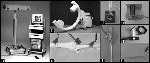
The navigated instruments (Figure 1) can be divided into three main groups according to functionality. The first group includes a calibrated fluoroscopic C-arm, a tool for measuring the gravitational direction, an accuracy checker for the verification of system accuracy, and a pointing device (pointer) for percutaneous digitization. This group of instruments is used for image acquisition and landmark registration. The next group consists of a surgical oscillating saw and an osteotomy chisel. These tools are used for cutting the bone. The final group includes three dynamic reference bases (DRBs), which are affixed to the femur, tibia, and proximal fragment of the tibia using 2.8-mm Kirschner wires. These are used to track the motion of the corresponding anatomy when the leg is flexed, extended, or rotated. All surgical instruments and DRBs can be gas- or steam-sterilized.

Figure 1. System components consist of (a) an optoelectric localizer and a computer system, (b) a registered fluoroscopic C-arm, (c) DRBs for tracking patient's anatomy, (d) a gravitational direction measurement tool, (e) an accuracy checker for the verification of system accuracy, (f) a pointer for percutaneous digitization, (g) a navigated saw, and (h) a navigated chisel for bone cutting.

The surgical procedure for using the system consists of the following steps: (1) image acquisition and landmark registration, (2) deformity measurement, (3) planning of the cutting plane and wedge size, and (4) navigational guidance of the osteotomy and wedge opening.

Image acquisition and landmark registration

The anatomical landmarks are registered intra-operatively for the representation of surgical objects and calculation of clinical parameters. A previously introduced hybrid concept [29] has been adapted to our system. It involves kinematic pivoting movement [30], percutaneous digitization using a pointer [30], and fluoroscopic image-based bi-planar 3D point reconstruction [31].

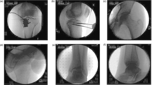
At the hip joint, the hip center [15] (H) is defined as the spherical center of the femoral head. This can be registered by either pivoting movement or bi-plane 3D point reconstruction using hip anterior–posterior (AP) and lateral images (Figure 2). When pivoting is used, a pointer is positioned at the ISAS (iliac spine anterior superior) of the pelvis to track the motion of the pelvis during the pivoting of the femur [30]. At the knee joint, the femoral posterior condyle axis [32] is defined as the line connecting the extreme points of the lateral and medial femoral posterior condyles. The tibial plateau is registered with the most lateral, medial, anterior, and posterior points at the tibial plateau edge using fluoroscopic bi-planar reconstruction from AP and lateral images of the knee. The knee center [15] (K) is defined as the center of the tibial plateau. At the ankle joint, the ankle center [15] (A) is defined as the middle point of the talus. This can be registered by using either fluoroscopic images or percutaneous digitization with a palpable pointer. In the latter case, the ankle center is calculated as the middle point of the trans-malleolar axis formed by the extreme points of the lateral and medial malleoli.

Figure 2. Fluoroscopic images used for landmark registration include (a) knee AP, (b) knee lateral, and optionally (c) hip AP, (d) hip lateral, (e) ankle AP, and (f) ankle lateral images.

Patient-specific coordinate system

Once the landmarks are registered, the patient-specific coordinate system can be established. For a mathematical description of bone and joint geometry, each articulate joint component needs its own coordinate system. On the femoral side, the frontal plane is defined as the plane that passes through the hip and knee centers and is parallel to the femoral posterior condyle axis. The sagittal plane passes through the hip and knee centers and is perpendicular to the frontal plane. The transversal plane is orthogonal to both the frontal and sagittal planes.

After the femoral coordinate system is established, the surgeons put the leg into a fully extended neutral position and transfer the lateral–medial (LM) direction from the femoral to the tibial side. The coordinate systems of the tibia and proximal fragment are then established with the knee, ankle center, and affined LM direction.

Functional parameters

Given all the landmarks, the functional parameters of the affected limb can be calculated. The femoral and tibial mechanical axes and the weight-bearing axis (the mechanical axis of the lower extremity) [33] are defined as the lines HK, KA, and HA, respectively. The varus/valgus angle is defined as the angle between the tibial and femoral mechanical axes in the frontal plane, and the flexion/extension angle is defined as the angle between them in the sagittal plane. The tibial plateau slope [33] is defined as the intersection angle of a line drawn from the anterior to the posterior edge of the tibial plateau and a second line perpendicular to the tibial mechanical axis lying in the sagittal plane. The deviation of the mechanical axis [33] is defined as the distance from the weight-bearing axis to the knee center at the frontal plane. With the registered width of the tibial plateau, the position of the weight-bearing axis at the tibial plateau coordinate can also be calculated [33].

The tibial and femoral joint lines [33] are defined as the lines tangential to the femoral distal condyles and the tibial plateaus. The medial proximal tibial angle [33] (MPTA) is then defined as the medial angle formed by the tibial joint line and the tibial mechanical axis.

Deformity measurement

The geometrical parameters of the affected limb are measured intra-operatively. They include varus angle, flexion angle, tibial plateau slope, and MPTA. There is no reliance on information derived from conventional full-leg X-ray images because either malrotation of the lower extremity or distortion of the image caused by parallax may introduce error [15–17].

Checking the soft tissue balance is very important [6]. Anatomical abnormalities include not only the primary varus, referring to the tibio-femoral osseous geometry, but also the secondary varus, resulting from the separation of the lateral tibiofemoral compartment due to soft tissue deficiencies. It is important to differentiate between these two because only the primary deformity should be corrected with the osteotomy [6]. With the help of the joint line convergence angle (JLCA) [34], which is defined as the intersection angle of the tibial and femoral joint lines in the frontal plane (Figure 3), surgeons can check osseous deformities along with any other ligament laxity by applying varus, valgus, and upward stresses to the tibia [35].

Figure 3. Femoral and tibial joint lines and JLCA. A biased JLCA value indicates that the deformity measured consists of not only a primary osseous deformity but also a secondary deformity resulting from lateral soft tissue laxity. In this case, the soft tissues need to be balanced. The normal range of JLCA lies between 0.7 and 2.4° according to Paley et al. [34].

Intraoperative planning

Planning of osteotomy plane

Fluoroscopic images aid planning of the osteotomy, including the determination of the position and orientation of the cutting plane in the frontal and sagittal planes. The cutting plane is superimposed on the fluoroscopic images to help the surgeon make a decision based on clinical factors such as geometry of the deformity, type of fixation, soft tissue coverage, bone quality, and so on. The adjusted parameters consist of directions in the frontal and sagittal planes, distance to the tibial plateau, osteotomy length, and the start and end points of the osteotomy.

Planning of wedge size

With conventional methods, the wedge size is planned using full-leg X-ray images, together with a color pen, goniometer, and scissors. Manual planning in this manner is difficult because the appropriate wedge size is dependent not only on the amplitude of deformity but also on the position of the osteotomy plane and the patient's anatomical size [14]. In addition, the conventional full-leg X-ray image is inaccurate, as we have described earlier. Therefore, an intuitive planning interface is provided, which helps the surgeon to determine the optimal wedge size and to predict the clinical outcome intra-operatively.

For the correction of a pure frontal plane deformity (Figure 4), which is the most common case in HTO, the appropriate wedge size, corresponding over-correction angle, and increment of leg length are automatically computed after the surgeon specifies the target position of the weight-bearing axis. For example, for the uni-compartmental osteoarthritis of grades I and II, the target position of the weight-bearing axis is 62.5% at the coordinate of the tibial plateau [6] (0% corresponds to the medial border and 100% corresponds to the lateral border), which approximates about a 3° valgus over-correction.

Figure 4. For the correction of frontal plane deformity, wedge size is determined according to the target position of the weight-bearing axis, where H is the hip center, A the ankle center, T the target position of the weight-bearing axis, P the position of the hinge axis, G the anticipated postoperative position of the ankle center, and α the wedge size [14].

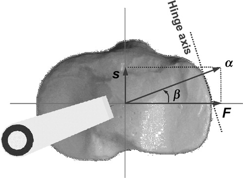
For complex multi-planar deformities, which exist in both the frontal and sagittal planes, the wedge has to be internally or externally rotated to correct with a single cut [14]. The rotation angle can be calculated after the surgeon defines the wedge size in the frontal and sagittal planes. For example, for the correction of a varus deformity together with recurvatum, the wedge is rotated internally (Figure 5); whereas for the correction of varus deformity together with hyperextension, the wedge is rotated externally.

Figure 5. The wedge is internally rotated to correct complex deformities that consist of varus deformity in the frontal plane and recurvatum in the sagittal plane, where F is the necessary wedge size in the frontal plane for the correction of varus deformity and S the wedge size in the sagittal plane for the correction of recurvatum. The overall wedge size is α, while the necessary internal rotation angle is β.

Navigational guidance

Bone cutting

The importance of an accurate osteotomy cannot be overemphasized. The intact lateral cortical bone hinge is vital for the stability and maintenance of the correction; therefore, penetration of the lateral cortex should be avoided. Inaccurate surgical techniques such as poor lateral visualization, under-estimation of saw blade depth, or incorrect determination of osteotomy length may cause this problem. Tibial plateau fractures [5], which can result from an inappropriate osteotomy having insufficient proximal fragment thickness, an incomplete bone cut, or unintentional supper-lateral obliquity of the saw blade, should also be avoided. Additionally, damage to the neurovascular structures may occur if the osteotomy is excessive on the tibial dorsal side.

Osteotomy guidance (Figure 6) is therefore provided to avoid these intra-operative pitfalls. With on-the-fly visualization, the position and direction of instruments can be simultaneously monitored in multiple fluoroscopic images. During osteotomy, the surgeon is able to monitor continuously the incisions made by the instruments. With real-time feedback of the distance from the instrument tip to the planned cutting plane and to the lateral cortical hinge, a safe and accurate osteotomy can be achieved.

Figure 6. Osteotomy is performed under navigational guidance. The incision of the instrument (e.g., a TomoFix® chisel, which is depicted as thin red lines for the contour and a green polyhedron for the tip) and deviation from the planned cutting plane (depicted as a blue line for the direction in the frontal plane and a red line for the direction in the sagittal plane) can be monitored in multiple fluoroscopic images. [Color version available online]

Wedge opening

The wedge is opened under navigational guidance. This is the most crucial and difficult step because once the wedge has been opened and the implant is in place, little can be done to make adjustments toward the ideal anticipated correction. An excessive or insufficient opening at the osteotomy site, particularly an asymmetrical opening, may introduce an unwanted secondary deformity, which can be either malrotation in the transversal plane or alteration of the tibial plateau slope in the sagittal plane. Until now, no reliable intra-operative method exists for the verification of wedge size, orientation, and axial alignment.

With our proposed navigation system, however, surgeons are provided with complete feedback of wedge size, wedge orientation, and axial alignment. When the wedge is opened, the system allows surgeons to analyse continuously and monitor the progress of the deformity correction. The 3D wedge is decomposed into three components in the frontal, sagittal, and transversal planes. These components are then compared with the respective planned values using sliders (Figure 7). In this way, any unintentional asymmetric openings can be observed and corrected. The axial alignment, joint line orientation, and intersection point of the weight-bearing axis with the tibial plateau are also navigated. These parameters provide the surgeon with a comprehensive view of the clinical outcome, thus enabling him/her to perform the planned procedure accurately.

Figure 7. The wedge is opened under navigational guidance. The navigated parameters include (a) components of the wedge size in the frontal, sagittal, and transverse planes, shown at the bottom of the window, (b) collinear parameters including varus/valgus angle, extension/flexion angle, and internal/external rotation angle of the tibia in relation to the femur, (c) tibial plateau slope, (d) MPTA. The position of the weight-bearing axis at the tibial plateau coordinate is shown in the upper right of the window. A 3D view of the wedge and mechanical axes is shown in the upper left. [Color version available online]

In vitro plastic bone validation

The proposed system was first validated in the laboratory environment with a plastic bone model, to establish the accuracy and precision in terms of inter-observer repeatability, intra-observer reproducibility, and end-to-end application accuracy.

Plastic bone model and test bench

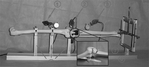
The plastic bone model was created using a normal entire leg model (RR0119, Synbone AG, Davos, Switzerland). The proximal and distal parts of the tibia were cut through and connected with a rubber hinge after removing a wedge along the AP and LM directions, respectively (Figure 8). Thus, a juxta-articular tibial deformity could be simulated. The plastic bone was then mounted on a test bench with multi-freedom fixtures. The distal part of the tibia was connected to a measurement gauge through a spherical joint, with which the position of the distal tibia could be measured.

Figure 8. Test bench used for the evaluation of application accuracy, which consists of (1) the DRB of the femur, (2) the DRB of the proximal fragment, (3) the DRB of the tibia, (4) multi-freedom fixtures, (5) a measurement gauge that enables free movement of the distal tibia inside the frame, (6) rulers used to measure the position of the distal tibia, and (7) spherical joint used to connect the distal tibia with the measurement gauge.

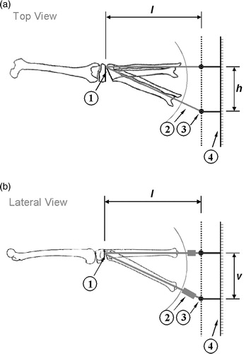
Uni- or multi-planar deformities could be created by moving the distal tibia relative to the proximal fragment. If it was moved horizontally, a pure frontal plane varus deformity was created (Figure 9a); if moved vertically, a sagittal plane deformity was created (Figure 9b). If the horizontal movement was combined with the vertical movement, multi-planar complex deformities, which existed in both the frontal and sagittal planes, were created.

Figure 9. Schematics of (a) top view and (b) lateral view of test bench, which include (1) hinge axis, (2) adjustable-length tube, (3) sphere joint, and (4) rulers. The CORA (center of rotation of augulation) of the created deformity is located at the position of the lateral hinge axis; the amplitudes of the deformity in the frontal and sagittal planes are θ_frontal = tan⁻¹(h/l) and θ_sagittal = tan⁻¹(v/l) respectively, where h and v are the amplitudes of the movement of the distal tibia in the horizontal and vertical directions and l is the distance between the position of the lateral hinge axis and the spherical joint.

Inter-observer repeatability

To evaluate the robustness when landmarks are registered with different operators, sets of 11 repeated measurements were made by five independent operators with identical experimental conditions. The inter-observer repeatability was defined as the consistency of the individual positions of landmarks and the functional parameters registered with each operator.

Each of the five operators possess different skills. Operator 1 had extensive clinical experience as well as knowledge of computer-assisted navigation systems. Operator 2 also had significant clinical experience but limited familiarity with navigation software. Operator 3 was an orthopedic specialist but with limited surgical experience and no experience with navigation software. Operators 4 and 5 had extensive experience with navigation software but no clinical experience.

The reference positions of landmarks were directly digitized on the plastic bone model by each of the five operators with a palpable pointer. Each operator repeated the procedure five times for each landmark. The ground truth landmark position was defined as the mean position of these repeated measurements.

Intraobserver reproducibility

The bi-planar 3D point reconstruction involved an AP and a lateral fluoroscopic image. The accuracy of this approach can be up to sub-millimeter based on phantom evaluation [31]. However, intra-operatively, it is cumbersome, and sometimes even impossible, to obtain accurate AP and lateral fluoroscopic images. The misalignment of the C-arm orientation may make the projected representation of the anatomical structure difficult to interpret and therefore potentially introduce registration error.

To assess such errors, five images of the knee joint were acquired in both the AP and lateral directions. The set of images acquired consisted of one well-aligned and four misaligned images. The four misaligned images were obtained with the C-arm rotated 10° towards the proximal, distal, lateral, and medial directions, respectively, in relation to the well-aligned image. The well-aligned AP image was obtained with the patella projected at the center of the femoral condyles; and the well-aligned lateral image was obtained with the lateral and medial femoral condyles overlapping each other. In a previous cadaver study, Wright et al. [17] demonstrated that the accuracy of achieving the true knee forward position by using the patella as a reference was within 5°. Therefore, we believe that a 10° misalignment can simulate the worst clinical situation.

The landmarks were then registered using 25 pairs of images formed from these five AP and five lateral images. One operator reconstructed all the landmarks, resulting in a total of 11 × 25 values. The intraobserver reproducibility was defined as the consistency of registered landmarks and functional parameters.

End-to-end application accuracy

The overall application accuracy was evaluated with the test bench. First, the neutral position of the plastic bone model, with both the varus/valgus and extension/flexion angles equal to zero, was adjusted and recorded by the computer. Then, with the movement of the distal tibia, uni-planar varus or multi-planar complex deformities were created, which were then measured by the navigation system. Optimal wedge size was planned, with the aim of correcting the created deformity and restoring the plastic bone model to the registered neutral position. After simulated HTO under navigational guidance, the residual and/or newly introduced secondary deformity was measured in relation to the registered neutral position. Five repeated interventions were performed with each created deformity. The end-to-end application accuracy was defined as the mean value of residual and/or newly introduced secondary deformity.

Preliminary clinical trial

The preliminary clinical trial began following the encouraging results obtained from the in-laboratory plastic bone evaluation. From June to August 2003, four patients (two men and two women) with osteoarthritis or varus deformity were operated on with the proposed navigation system by one author (P.K.). The average age of the patients at the time of operation was 40.8 years (range: 23–55 years). All patients received medical opening valgus osteotomy using the TomoFix® technique.

The use of ultrasound as a reliable and accurate 2.5D tool for the registration of patient anatomy has been previously described and introduced in a clinical setting [25]. Although our proposed system actually does not need preoperative planning, we still used the ultrasound system to measure the preoperative deformity and postoperative axial alignment in our primary clinical trial for the purpose of verification. The measurements made using the ultrasound system were compared with those made with the navigation system.

Results

In vitro plastic bone evaluation

Inter-observer repeatability

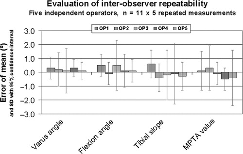
Despite the differences in surgical experience and knowledge of the navigation system, there was complete consistency among all the operators in the registration of all the landmarks, and therefore also in the calculation of the clinical parameters. The maximum inter-observer difference of mean value was found to be 0.3° for varus, 0.6° for flexion, 1.0° for tibial plateau slope, and 0.8° for MPTA, with standard deviations (SD) (95% confidence interval) of 0.8, 1.2, 1.6, and 1.2°, respectively (Figure 10). The maximum discrepancy between the mean value and the reference value was 0.5° for varus angle and 0.6° for flexion angle. The SD (95% confidence interval) of the position of the weight-bearing axis at the tibial plateau coordinate was found to be 3.1%, with a maximum inter-observer difference of 2.8%.

Figure 10. The inter-observer repeatability of functional parameters was evaluated by five independent operators under identical experimental conditions.

Intra-observer reproducibility

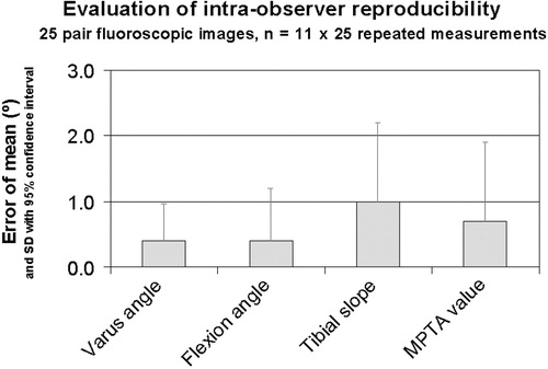
With 25 pairs of images acquired in the well-aligned and misaligned positions, the landmarks were registered and functional parameters were calculated. The mean deviation was found to be 0.4° for varus, 0.4° for flexion, 1.0° for tibial plateau slope, and 0.7° for MPTA, with an SD (95% confidence interval) of 0.6, 0.8, 1.2, and 1.2°, respectively (Figure 11). The maximum deviations were 0.9° for varus, 1.1° for flexion, 2.0° for tibial plateau slope, and 2.1° for MPTA. The mean discrepancy of the position of the weight-bearing axis at the tibial plateau coordinate was 1.1%, with an SD (95% confidence interval) of 2.5%.

Figure 11. The intraobserver reproducibility of functional parameters was evaluated with 25 pairs of fluoroscopic images. All measurements, i.e., 11 repeated measurements for each image pair, were performed with one operator.

End-to-end application accuracy

For the HTO interventions performed on the uni-planar varus deformities (2.5, 5.0, 7.5, and 10° varus) created with the test bench, we found that the mean value of residual and/or newly introduced deformities of all trials was 0.4°, with a maximum value of 1.1°.

For the multi-planar complex deformities, which consisted of a 10° varus deformity in the frontal plane together with a 2.5, 5.0, 7.5, or 10° recurvatum in the sagittal plane, the mean value of residual and/or newly introduced deformities was found to be 0.4° in the frontal and 0.5° in the sagittal plane, with a maximum error of 0.9 and 1.4°, respectively.

Preliminary clinical trial

All four patients had a varus deformity that ranged from 5.0 to 8.0° prior to the operation. After the operation, the weight-bearing axis of the affected limb was moved from the medial to the lateral compartment in every patient. The target position was determined by the surgeon according to clinical factors [2].

All operations were successfully supported by the navigation system. No complications were found in any patient. The average extra OR time was 30–40 min. This was mainly attributed to the fixation of DRBs, acquisition of the fluoroscopic images, and the positioning of the Optotrac® camera. However, there was a fast learning curve associated with these extra procedures, which meant that the amount of extra OR time required could be quickly reduced.

All deformities were accurately corrected. When compared with the measurements made from the ultrasound system, the mean error was found to be 1.0°, with a maximum error of 2° in all patients (Table I).

Table I.  Preoperative deformity and postoperative axial alignment in preliminary clinical trial.

				Preoperative		Postoperative
Number	Diagnosis	Age	Gender	Ultrasound	Navigation	Navigation	Ultrasound
1	Posttraumatic gonarthrosis	39	M	8° varus	7° varus	2° valgus	2° valgus
2	Medial gonarthrosis	55	W	7° varus	7° varus	0°	1° valgus
3	Genu varum	23	W	4° varus	5° varus	0°	1° varus
4	Posttraumatic gonarthrosis	46	M	7° varus	8° varus	0°	2° valgus

Discussion

Landmark registration method

Hip center

Theoretically, the pivoting algorithm is sufficiently accurate [36]. However, many factors may limit the clinical practicality of this method, such as limited range of motion, patient obesity, or a non-spheroid femoral head. In addition, patients with severe dysplasia, ankylosis, or any other abnormalities of the hip joint are probably not practical candidates for such surgical procedures [36]. In these cases, the hip center should be registered with fluoroscopic images, which, in our plastic bone evaluation, proved to be more accurate and reproducible than the pivoting algorithm. However, in this case, two additional fluoroscopic images, which are unnecessary with the pivoting algorithm, need to be acquired at the hip joint.

Ankle center

Several previous studies [37], [38] have explored the registration accuracy of the ankle center based on percutaneous digitization. Our plastic bone evaluation confirms that digitization of the extreme point at the lateral and medial malleoli is a simple and reliable method. However, if a patient is too obese to palpate the malleolus or if a deformity exists at the ankle joint, bi-planar fluoroscopic reconstruction should be used.

Knee center

Moreland et al. [15] have previously evaluated the different geometric methods for defining the knee center in the frontal plane. They reported that the result is approximately the same when using the top of the femoral notch, the middle point of the femoral condyles, the center of the tibial spines, or the center of the tibial plateau. However, no publication has addressed the reliability and reproducibility of registration when bi-planar fluoroscopic reconstruction is used.

We found that the edges of the lateral and medial tibial plateaus are the most reproducible landmarks when compared with other landmarks such as the tibial spines or femoral notch. The reason for this is that they can be unambiguously and objectively identified by the surgeon in the fluoroscopic images. However, if the acquired images are misaligned, which may happen in the clinical situation, the registered position differs significantly due to the misinterpretation of the 2D projection of the 3D anatomic structure of the tibial plateaus (Figure 12). We found that, in the previously described 25 image pairs, the Euclidean distance between the maximum and minimum positions was 5.0 mm in the LM direction and 13.9 mm in the AP direction. This corresponds to an angular deviation of 1.5 and 3.9° in the LM and AP directions, respectively.

Figure 12. The registration errors of the knee center resulting from the image misalignment tend to cancel each other out. The lateral and medial tibial plateau edges registered with well-aligned AP and well-aligned lateral images are points 1 and 2; whereas they are points 3 and 4 if registered with misaligned AP and well-aligned lateral images, and they are points 5 and 6 if registered with misaligned AP and misaligned lateral images. However, the knee center (black sphere), which is defined as the center of the tibial plateau, i.e., the middle point of the lateral and medial tibial plateau edges, is approximately at the same position.

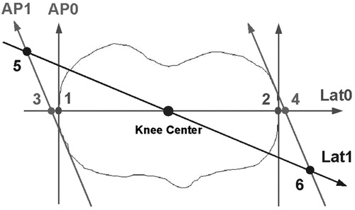
Nevertheless, these errors tend to cancel each other when the knee center is calculated as the middle point of the tibial plateau. This is due to the symmetrical shape of the tibial plateau along the LM direction (Figure 12). We found that the maximum discrepancy with the reference point is only 1.5 mm in the frontal plane and 2.9 mm in the sagittal plane, which corresponds to angular deviations of 0.5 and 0.9°, respectively.

Mathematical simulation

A mathematical simulation was used to estimate the mean error of the application in the normal case and the maximum deviation in the worst-case scenario.

On the basis of the mean position and SD of each landmark obtained from the plastic bone evaluation, the randomized points were generated for each landmark according to the normal distribution using the polar form of the Box–Muller transformation [39]—100 points were generated for each landmark. After statistical analysis of all data combinations, the application accuracy with 95% confidence interval which reflects the normal case and maximum error in the worst-case scenario can be estimated.

We found that the mean error was 0.7° for the varus angle and 0.9° for the flexion angle, with an SD (95% confidence interval) of 1.0° for the varus angle and 1.4° for the flexion angle. In the worst-case scenario, the maximum deviations of the varus and flexion angles were 2.6 and 3.6°, respectively. However, this corresponds to a possibility of <0.1%.

Any discussion of accuracy would be incomplete without mentioning the clinical requirement [40]. Retrospective clinical studies have suggested that the goal of HTO is to obtain the axial alignment of the lower extremity in the frontal plane within a narrow range of ±2° to expect good long-term result [6]. Our mathematical simulation suggests that the clinical outcomes will be within this critical region with a probability >95%.

Wedge opening: conventional approach vs. CAS

Wedge opening is a critical procedure that involves not only the control of the wedge size but also the correct placement of the hinge axis and the correct wedge orientation.

The accurate placement of the lateral hinge axis is important. Placing the axis too far medially can make the opening procedure difficult or, even worse, result in fractures of the tibial plateau, whereas placing the axis too far laterally will disrupt the lateral cortex bone, possibly resulting in instability of the fixation during healing.

The orientation of the wedge is also very important because the asymmetrical opening of the wedge would introduce an unwanted secondary deformity. For example, an asymmetrical opening at the AP direction would change the tibial plateau slope, which may result in anterior or posterior instability due to excessive posterior or anterior slope [5].

An important clinical advantage of the computer-assisted navigation system is accurate control of the hinge axis and wedge orientation. With on-the-fly visualization of projections of the instruments, the position of the hinge axis can be accurately controlled. With real-time feedback of wedge components in frontal, sagittal, and transversal planes, any mis-orientation of the wedge can be observed and corrected.

In contrast, with conventional techniques, the surgical plan is derived from only the frontal plane X-ray film. Thus, there is an assumption that the hinge axis is always perpendicular to the frontal plane. The intended kinematics of the plan will be reproduced in the theater only if this assumption holds true. Therefore, if the hinge axis is somewhat rotated, which is possible as surgeons do not have an effective way to control the wedge orientation, the correction obtained in the frontal plane will not be the one anticipated. Furthermore, an unwanted alteration of the tibial plateau slope in the sagittal plane or an internal/external rotation of the tibia in the transversal plane may be introduced. This can explain certain errors in the postoperative outcome, even if the preoperative planning was accurate.

Future plan

Currently, a multi-center clinical study is underway to evaluate the long-term clinical benefits of the system. From the application point of view, the current software only supports the opening wedge tibial osteotomy. However, we are already in the progress of extending the current module to include focal dome [41] and closing wedge [42] osteotomies on the tibial side, as well as femoral [43] and double [44] osteotomies. It should be noted that the latter is very difficult to correct with conventional techniques.

Conclusions

A CT-free computer-assisted navigation system for high tibial opening wedge osteotomy has been proposed and successfully introduced into operating theaters. The system allows surgeons to accurately measure the deformity, interactively plan the surgical procedure, and precisely perform the osteotomy under navigational guidance. This system is substantially different from other computer-assisted approaches for osteotomy planning or robotic preparation, as it does not require any preoperative procedure or alteration of the conventional surgical procedure; neither does it require any information derived from full-leg X-ray images.

In conclusion, although complications in HTO may occur, they can be eliminated or minimized with computer-assisted navigation techniques. The intra-operative planning and navigational guidance provided by our proposed system reduces the risk of complications and increases the safety, accuracy, and reproducibility, and thus improves the clinical outcome of this surgical procedure.

Acknowledgment

The authors acknowledge Dr M. Kunz for her help during the beginning of the project, Mr U. Rohrer for his help in manufacturing the test bench, and Mr B. Ebert and Mr B. Blake for their help with the preparation of the manuscript. The financial support of the AO/ASIF Foundation, Davos, Switzerland, the M.E. Müller Foundation, Bern, Switzerland, the Swiss National Science Foundation (NCCR/CO-ME), and PRAXIM MediVision, La Tronche, France is gratefully acknowledged.

References

- Coventry M B, Minnesota R. Osteotomy about the knee for degenerative and rheumatoid arthritis. JBJS. 1973; 55A: 23–48
- Müller W. High tibial osteotomy, conditions, indications, techniques, problems. 2001; 28: 194–204, European Federation of National Associations of Orthopaedics and Traumatology
- Murphy S B. Tibial osteotomy for genu varus: indications, preoperative planning, and technique. Orthop Clini North America 1994; 25: 477–482
- Handal E G, Morawski D R, Santore R F. Complications of high tibial osteotomy. Knee Surgery, F H Fu, C D Harner, K G Vince. William & Wilkins, Baltimore, MDUSA 1996
- Phillips M J, Krackow K A. High tibial osteotomy and distal femoral osteotomy for valgus or varus deformity around the knee. AAOS Instructional Course Lecture 1998; 47: 429–436
- Noyes F R, Barber-Westin S D, Hewett T E. High tibial osteotomy and ligament reconstruction for varus angulated anterior cruciate ligament-deficient knees. Am J Sport Med 2000; 28(3)282–293
- Hernigou P, Ma W. Open wedge tibial osteotomy with acrylic bone cement as bone substitute. Knee. 2001; 8: 103–110
- Magyar G, Ahl T, Vibe P, Toksvig-Larsen S, Lindstrand A. Open-wedge osteotomy by hemicallotasis or the closed-wedge technique for osteoarthritis of the knee, a randomized study of 50 operations. J Bone Joint Surg Br 1999; 81(3)444–448
- Staubli A, De Simino C, Babst R, Lobenhoffer P. TomoFix: A new LCP-concept for open wedge osteotomy of the medial proximal tibia—early results in 92 cases. Injury Int J Care Injured 2003; S-B55–S-B62
- Koshisa T, Murase T, Saito T. Medial open wedge high tibial osteotomy with use of porous hydroxyapatite to treat medial compartment osteoarthritis of the knee. JBJS. 2003; 85A: 79–85
- Naudie D, Bourne R, Rorabeck C, Bourne T. Survivorship of the high tibial valgus osteotomy. CORR 1999; 367: 18–27
- Rudan J F, Simurda M A. Valgus high tibial osteotomy. CORR 1991; 268: 157–160
- Sprenger T R, Doerzbacher J F. Tibia osteotomy for the treatment of varus gonarthrosis. J Bone Joint Surg 2003; 85A: 469–474
- Dahl M T. Preoperative planning in deformity correction and limb lengthen surgery. AAOS Instructional Course Lecture 2000; 49: 503–509
- Moreland J R, Bassett L W, Hanker G J. Radiographic analysis of the axial alignment of the lower extremity. JBJS. 1987; 69A: 745–750
- Jiang C, Install J N. Effect of rotation on the axial alignment of the femur. CORR 1989; 248: 50–56
- Wright J G, Treble N, Feinstein A R. Measurement of lower limb alignment using long radiographs. JBJS 1991; 73B(5)721–723
- Puddu G, Franco V. Femoral antivalgus opening wedge osteotomy. Oper Tech Sport Med 2000; 8(1)56–60
- Fowler P J, Tan J L, Brown G. Medial opening wedge high tibial osteotomy: how I do it. Oper Tech Sport Med 2000; 8(1)32–38
- Staubli A E, De Simoni C, Sukthankar A. Aufklappende hohe interligamentäre Tibiavalgisations-Osteotomie (HTO) ohne Interponat mit TomoFix (in German). 2001, Expert meet Expert 74, AO course, Davos, Switzerland
- Chao E Y, Sim F H. Computer aided preoperative planning in knee osteotomy. Iowa Orthop 1995; 15: 4–18
- Tsumura H, Himeno S, Kawai T. The computer simulation on the correcting osteotomy of osteoarthritis of the knee. J. Jpn Orthop Assoc 1984; 58: 565–566
- Lin H, Birch J, Samchukov M, Ashman R. Computer assisted surgery planning for lower extremity deformity correction by the Ilizarov method. J Img Guided Surg 1995; 1: 103–108
- Kawakami H, Sugano N, Nagaoka T, Hagio K, Yonenobu K, Yoshikawa H, Ochi T, Hattori A, Suzuki N. 3D analysis of the alignment of the lower extremity in high tibial osteotomy. Proceedings of Medical Image Computing and Computer-Assisted Intervention (MICCAI 2002), TokyoJapan, September 2002. Springer, Berlin 2002; 261–267
- Keppler P, Strecker W, Kinzl L, Simnacher M, Claes L. Die sonographische Bestimmung der Beingeometrie. Orthopade 1999; 28: 1015–1022
- Ellis R E, Tso C Y, Rudan J F, Harrison M M. A surgical planning and guidance system for high tibial osteotomy. Comput Aided Surg 1999; 4: 264–274
- Phillips R, Hafez M, Mohsen A, Sheman K, Hewitt J, Browbank I, Bouazza-Marouf K (2000) Computer and robotic assisted osteotomy around the knee. Proceedings of MMVR 2000—8th Annual Medicine Meets Virtual Reality Conferenc, Newport Beach, CA, January, 2000. IOS Press, Amsterdam, 265–271
- Sargaglia D, Pradel P, Chaussard C, Liss P. OrthoPilot® assisted valgus osteotomy in osteoarthritic genu varus—results of the axial correction in a case-control study of 56 cases. Proceeds of Computer Assisted Orthopaedic Surgery (CAOS, MarbellaSpain. F Langlotz, B L Davies, A Bauer. 2003; 314
- Zheng G, Marx A, Langlotz U, Widmer K, Buttaro M, Nolte L P. A hybrid CT-free navigation system for total hip arthroplasty. Comp Aided Surg 2002; 7: 129–145
- Kunz M, Strauss M, Langlotz F, Deuretzbacher G, Rüther W, Nolte L P. A non-CT based total knee arthroplasty system featuring complete soft-tissues balancing. Proceedings of Medical Image Computing and Computer-Assisted Intervention (MICCAI 2001), UtrechtNetherlands. Berlin, October 2001, 409–415
- Hofstetter R, Slomczykowski M, Krettek C, Koppen G, Sati M, Nolte L P. Fluoroscopy as an imaging means for computer assisted surgical navigation. Comp Aid Surg 1999:; 4: 65–76
- Arima J, Whiteside L, McCarthy D, White S E. Femoral rotation alignment: based on the anteriorposterior axis in total knee arthroplasty in a valgus knee. JBJS. 1995; 77A: 1331–1334
- Paley D. Principles of Deformity Correction. Springer-Verlag, BerlinHeidelberg, 2002; 480–483; 485–490
- Paley D, Herzenberg J E, Tetsworth K, McKie J, Bhave A. Deformity planning for frontal and sagittal plane corrective osteotomies. Orthop Clini North Am 1994; 25: 425–465
- Paley D, Bhatnagar J, Herzenberg J, Bhave A. New procedure for tightening knee collateral ligaments in conjunction with knee realignment osteotomy. Ortho Clini North Am 1994; 25: 533–555
- Stindel E, Gyl D, Briard J, Plaweski S, Lefevre C. Detection of the hip in computer assisted TKA: An evaluation study of the accuracy and reproducibility of the Surgetics algorithm. Proceedings of the Second Annual Conference on the International Society for Computer Assisted Orthopaedic Surgery (CAOS). 65
- Stindel E, Gyl D, Briard J, Merloz P, Dubrana F, Lefevre C. The center of the ankle in CT-less navigation system: what is really important to detect?. Proceedings of the Second Annual Conference on the International Society for Computer Assisted Orthopaedic Surgery (CAOS). 63
- Nofrini L, Slomczykowski M, Lacono F, Zaffagnini S, Marcacci M. Estimation of accuracy in ankle center location for tibial mechanical axis identification using computer assisted surgery system. Proceedings of the Second Annual Conference on the International Society for Computer Assisted Orthopaedic Surgery (CAOS). 67
- Box G, Muller M. A note on the generation of random normal deviates. Annals Math Stat 1958; 29: 610–611
- Simon D A. Frameworks for evaluating accuracy in CAOS. Proceedings of the First Joint CVRMed/MRCAS Conferenc, GrenobleFrance, March 1997. Springer, Berlin 1997; 195–197
- Sundaram N A, Hallet J P, Sullivan M F. Dome osteotomy of the tibia for osteoarthritis of the knee. JBJS. 1986; 68B: 782–786
- Billings A, Scott D. High tibial osteotomy with a calibrated osteotomy guide, rigid internal fixation, and early motion. JBJS. Camargo M., Hofmann A. 2000; 82A: 70–79
- Mathews J. Distal femoral osteotomy for lateral compartment osteoarthritis of the knee. Orthopaedics 1998; 21: 437–440
- Babis G, An K, Chao E, Rand J, Sim F. Double level osteotomy of the knee: A method to retain joint-line obliquity: clinical results. JBJS. 2002; 84A: 1380–1388