Virtual 3D planning and guidance of mandibular distraction osteogenesis

Abstract

We present a system for 3D planning and pre-operative rehearsal of mandibular distraction osteogenesis procedures. Two primary architectural components are described: a planning system that allows geometric bone manipulation to rapidly explore various modifications and configurations, and a visuohaptic simulator that allows both general-purpose training and preoperative, patient-specific procedure rehearsal. We provide relevant clinical background, then describe the underlying simulation algorithms and their application to craniofacial procedures.

• Surgical simulation
• surgical planning
• craniofacial surgery
• distraction osteogenesis

Introduction

Distraction osteogenesis

The treatment of patients with complex anatomical deformities caused by trauma or congenital defects is one of the most challenging multidisciplinary tasks in medicine. Due to the introduction of plating systems and changes in surgical technique in the last 20 years, correction of severe malformations has become possible. Such procedures are generally performed by highly specialized teams, frequently in a single operation.

Distraction osteogenesis is gaining popularity as a common treatment for facial deformities. Such procedures aim to lengthen and reform the diseased or damaged portion of the mandible by performing one or more osteotomies (surgically induced bone fractures), manipulating the resulting bone fragments into a more desirable configuration, and “growing” the mandible through daily distraction.

The precise planning of osteotomies, bone manipulations, and distraction for such procedures remains a difficult challenge, requiring the surgeon to balance the dual goals of functional rehabilitation and aesthetic outcome. The skull, facial bones, maxilla, mandible and overlying soft tissues must all be manipulated to achieve the optimal result, and implantation of autologous or foreign material is often required to replace missing tissue. As disturbances of craniofacial integrity are highly visible, optimal results in restoration are extremely important in these patients. Planning is further complicated by the necessity to adhere to a distraction plan of anatomically feasible daily bone growth to avoid premature fusion or nonunion of the bone.

Clinical relevance

In the United States alone, approximately 3 million people present to the emergency room with traumatic facial injuries annually. Motor vehicle accidents (MVAs) were the most frequent cause of facial injuries prior to 1970. However, the number of violence-, job- and sports-related and self-inflicted injuries has risen – contributing to a fairly constant number of facial injuries despite a decrease in MVA-related facial trauma. In a large retrospective study of 2137 patients [1], mandibular fractures were caused by vehicular accidents (43%), assaults (34%), work-related accidents (7%), mechanical falls (7%), sporting accidents (4%), and miscellaneous trauma (5%). Most facial injuries involve both bone and soft tissue, which are deformed due to direct impact. Similarly, children born with congenital deformities of the head and neck and cancer patients after removal of head and neck tumors require reconstructive surgery for rehabilitation. Due to the complex anatomy, critical functional requirements, and high visibility, facial reconstructive surgery in these patients is a challenging enterprise.

Virtual planning

The goal of a surgical plan in reconstructive surgery is the normalization of the shape, symmetry, dimension, and function of hard and soft tissue. At present, surgical plans and surgical outcomes are analyzed on 2D and 3D radiographs and photographs. As much of the challenge in trauma surgery lies in understanding the relative spatial positions of critical vascular, neural and other structures in relation to the underlying bone and the facial surface, recent developments in imaging techniques have allowed more effective pre-surgical diagnosis and surgical planning using patient-specific data.

Recently, research emphasis has also been placed on computer-assisted surgical planning and augmentation systems. State et al. [2] have developed an augmented reality system for ultrasound-guided needle biopsy of the breast. The system is used both for training and for intraoperative augmentation. The same group has also developed a similar system for laparoscopic training and augmentation. Other simulation projects have focused on training for laser iridium procedures [3], arthroscopy [4], intraocular surgery [5], and craniofacial implant design [6].

The virtual planning work presented here builds more specifically on previous work on craniofacial surgical planning and the diagnostic prediction of surgical outcomes [7–10].

Our work on visuohaptic simulation of surgical procedures builds on previous work in the simulation of bone surgeries, with relevant adaptations to craniofacial surgery and to our planning environment. Previous work on haptic simulation of bone surgery has focused largely on temporal bone surgery [11–14], with some work on other procedure categories, e.g., arthroscopy [15]. Preliminary work on the haptic simulation of craniofacial surgery is presented in reference 16.

Project description

The numerous functional and aesthetic constraints to which craniofacial surgeries are subject require precise preoperative planning. The work presented here aims to allow “trial and error” surgery to be carried out before ever entering the operating room. A geometric planning component allows the surgeon to rapidly experiment with various bone manipulations and plate/distractor configurations, and an interactive simulator component with haptic feedback allows the surgeon to “practice” the procedure on a patient-specific model. This system provides the surgeon with a significant advantage in preparing for procedures that are both technically challenging and difficult to plan.

This paper begins with a description of our interactive planning system, then discusses our force-feedback simulator, and concludes with a discussion of future work and the next steps toward intraoperative applications.

Virtual planning environment

Overview

We begin with a discussion of our interactive planning system, which allows the manipulation of real patient data before surgery and provides semi-automatic determination of a healthy template for a diseased mandible. The description uses the surgical correction of hemi-facial microsomia – a condition in which the mandible is unilaterally diseased and/or deformed – as a context and running example. Patients presenting with this condition are often considered candidates for distraction osteogenesis, so it is an appropriate example.

Planning for this condition also makes optimal use of the mirroring techniques incorporated into our system, which allow the surgeon to use a mirrored version of the healthy side of the mandible as a template for planning distraction for the diseased side. The distraction planning techniques discussed herein may be used in other cases as well, if both sides of the mandible are diseased or if the surgeon does not wish to use the healthy side as a template.

Data import

Preoperative head CT scans are converted into an isosurface representation using the Marching Cubes method [22]; this processing is done using the Amira software package (Mercury Computer Systems, Berlin, Germany). All subsequent processing uses isosurface data. The region of the isosurface corresponding to the mandible is labeled manually.

Symmetry plane definition

The first step in distraction planning for a patient with hemifacial microsomia is to define symmetry planes for the skull and the mandible. We use existing image registration techniques [17] to define a symmetry plane automatically for the skull [18], [19].

The surgeon then visually defines what is believed to be the center plane of the mandible. This is difficult to perform automatically at present, given the expected asymmetry in the image data due to unilateral malformation. The healthy half of the mandible is then “mirrored” by determining the distance of each point on the healthy side from the defined center plane and replicating that point on the opposite side of the center plane. The “healthy template” thus contains copies of all points from the healthy side of the mandible. Figures 1a and 1b depict the diseased mandible and the mandible with the mirrored portion included, respectively. From this point forward, the mirrored portion of the mandible serves as a template for the surgeon in defining the distraction of the diseased portion of the mandible.

Figure 1. Diseased mandible (left) and mirrored healthy template (right). [Color version available online.]

Once the symmetry planes for the skull and mandible are known, the skull, original mandible, and healthy template for the diseased mandible may be displayed on the screen in a semi-transparent or wireframe mode. Figure 2 shows the skull and the mandible, with the healthy template superimposed semi-transparently on the diseased mandible, as the surgeon would see it when using the planning system.

Figure 2. The healthy template is shown semi-transparently in blue. The mandible is shown in white. The midsagittal plane is indicated in red. [Color version available online.]

Performing the virtual operation

Once the healthy template for the mandible has been established, the surgeon can perform the first stages of the virtual operation. The decision regarding osteotomy location is one of the critical phases in planning corrective surgery for hemifacial microsomia. Using a series of geometric and analytic tools, controlled via the mouse, the surgeon is able to induce “fractures” in the surface model, implemented as the introduction of discontinuities in the triangular surface mesh used to represent the skull and mandible. More details on the algorithms used to perform these virtual cuts and identify the resulting discontinuities are presented in reference 20. These modifications can also be “rolled back”, allowing the surgeon to explore various operative approaches before proceeding to the next stage. Figure 3 shows examples of cutting bone using our system.

Figure 3. A planar cutting tool is used to graphically insert fractures in a surface model of the mandible. [Color version available online.]

Fragment positioning

Subsequent to fracture introduction, the surgeon independently manipulates separated bone fragments to explore various bone configurations. In general, the healthy template provides goal positions for the placement of each fragment. The surgeon does not necessarily have to follow the healthy template precisely; an exact match to the form of the healthy template will be impossible in most cases. However, using the healthy template, the surgeon may provide a plan for a reasonable outcome in terms of both form and function.

Automatic vector determination

The next stage is the placement of the distraction apparatus. Currently, a surgeon uses personal expertise to determine the path through which the bone will travel during distraction and the daily rate of distraction. This desired path must be translated into the position and orientation of the physical distractor. To provide the reader with a general orientation and a sense of scale, Figure 4 depicts an infant with a physical distractor.

Figure 4. A straight distractor used in vivo.

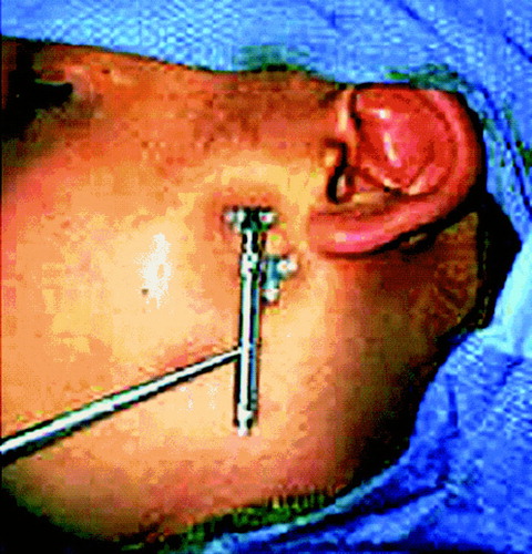
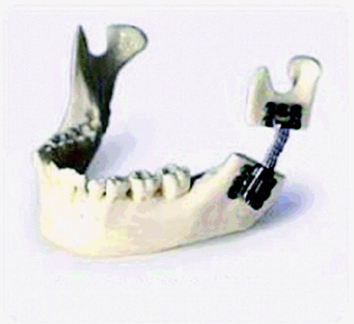
In some cases, the desired movement of the bone is restricted to translation – movement along a straight line in three dimensions. In this simple case, a standard distractor can be used and the distractor is advanced at a constant 1 mm/day. In many cases, however, anatomic constraints necessitate distraction along a curve in two or three dimensions (see Figure 5) and may also require rotations around one or more axes. In these cases, even for experienced surgeons, it is difficult to determine the precise trajectory over which the mandibular fragments should travel, and even more difficult to determine how to construct the distraction apparatus to effect that plan.

Figure 5. Distraction along a curve. Note that the edges of the bone along the osteotomy are no longer parallel.

Semi-automatic vector determination can reduce the complexity of the distraction planning process. Our simulation environment thus includes a module for automatic vector determination, which can generate a distraction plan based on the starting and desired positions of the bone. The output of this module includes (1) a path through which the bone should travel and (2) the rate at which the path should be traversed. The remainder of this section describes our approach to automatic vector determination.

Once the surgeon has specified the desired bone configuration (see Fragment positioning above), the automated vector determination algorithm defines a path and rate of advancement that will translate and rotate the bone into the goal configuration, subject to a maximum osteogeneration rate (typically 1 mm/day).

To determine the vector through which bone on two sides of a particular osteotomy must travel, we define a plane to represent each of the cut edges of the bone – that is, the two surfaces that “face each other” across the osteotomy – and determine the centroid of each bone fragment on those planes. These planes will not necessarily correspond to any particular physical surface along the cut, but will contain points from the cut bone or that approximate the orientation of the fractured edge. Figure 6 illustrates the plane and centroid derived from a fractured edge.

Figure 6. A fractured virtual bone surface and the plane derived from this surface. The plane is indicated in semi-transparent blue, with its centroid and surface normal indicated by the red vector. The three green points were used to generate the equation for this plane. [Color version available online.]

To identify the plane representing each cut surface, three non-collinear points on the cross-section of the bone are selected. These points can be determined automatically or may be selected by the surgeon. Greater distance between the points will, on average, reduce numerical error in the approximation of the bone surface, so the optimal set of points tends to lie at the extremes of the bone's cross-section. We have devised a method for automatically selecting points as follows:

• Determine the average location of all points along the cut; this average defines the “cut center”, C.

• Choose the first point P1 to include in the plane as the point that is furthest from C.

• Define a vector V from C to P1.

• For each point P′ on the cut surface, define a vector V′ from C to P′ and compute the angle α between V′ and V.

• Choose the second and third points (P2 and P3) to include in the planar approximation of the surface as those whose α values are closest to 120° and − 120° (Figure 7).

Figure 7. The selection of points from the cross-section of a virtual cut to determine a representative plane. C is computed as the centroid of all points on the cut surface, P1 is computed as the most distant point from C, and P2 and P3 are computed to generated angles of 120° and − 120° around C.

Although this does not always optimize the distribution of points, it runs quickly and provides an adequate point set. A more optimal (but more complex) approach would aim to maximize the area of the triangle defined by the three points.

Once the three points are established, the centroid of the representative plane is defined as the average of the three points. Given that most cuts will be planar or approximately planar, the plane defined by these three points will approximate the surface of the cut.

Note that in the case where the virtual fracture was induced using an analytic planar cut tool, the two sides of the cut will have the same shape and will contain the same points. Therefore, the points and centroid determined for one side of the cut can be used to define the centroid and plane for the other side.

Once the two planes for the two sides of the cut and the corresponding centroids have been established, the distraction plan can be generated, subject to several constraints. First, no point on the bone can be advanced more than 1 mm in a single day, as rapid distraction can cause soft tissue damage and inadequate bone reformation. Second, no point on the surface can travel backwards, as bone regrowth will occur within the distraction gap, as this is likely to cause premature fusion.

In the simple case of a straight-line distraction, these constraints are trivially satisfied, since all points along the osteotomy travel the same distance each day. However, when the distraction is performed along a curve, different points on the surface will travel different distances. The points along the outside of the curve will travel a greater distance than more “interior” points (those on the inside of the curve), and interior points may even travel backwards if a distraction step involves rotation of the bone (see Figure 8). Manually determining the movement of individual points along the path, to ensure that the key constraints are satisfied, is a time-consuming and imprecise task. Our system thus computationally ensures that these constraints are met when generating a distraction plan.

Figure 8. An example of “backtracking” in a distraction plan that may cause premature fusion. Here the dark lines indicate the position and orientation of the cut surface as it moved along the distraction trajectory. As a result of high curvature, the point at the end of the line has moved “backwards” relative to its previous position. [Color version available online.]

We represent our distraction plan as a Hermite curve, a 3D function that generates a smooth trajectory between two points, constrained by specified movement direction vectors at the beginning and end of the trajectory. In our case, the end points of the Hermite curve are the starting position and ending (goal) position of the distracted bone fragment's centroid. The starting and ending movement vectors are the normals of the distracted bone fragment's representative plane, before and after distraction. Figure 9 illustrates these values graphically on an example bone configuration, and Figure 10 demonstrates an example Hermite trajectory.

Figure 9. The points (P1, P2) and normals (R1, R2) are used to define a Hermite curve that represents the distraction plan. [Color version available online.]

Figure 10. An abstract representation of the smooth Hermite trajectory. Note that at P1 and P2, the curve's tangent is equal to R1 and R2, respectively.

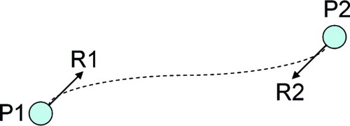
The Hermite curve is defined parametrically as:where t is a time value ranging from 0 → 1, p(t) is the position of the distracted bone fragment at time t, P1 is the initial position of the distracted bone fragment, P2 is the final position of the distracted bone fragment, R1 is the initial normal vector of the distracted bone fragment (as determined above), and R2 is the final normal vector of the distracted bone fragment [21]. Note that in this description, the “position” of a bone fragment refers to the position of the fragment's representative centroid, as defined above. Similarly, the “normal” of a bone fragment refers to the normal of the fragment's representative plane, as defined above.

The Hermite equation thus defines a movement trajectory for the distracted bone fragment. Note that the tangent to this curve at any point defines the orientation of the representative plane during distraction, so the Hermite curve specifies a rotation plan as well as a translation plan. It does not, however, specify any rotation around the axis of distraction. If the initial and final orientations of the representative plane around its normal are different, it is also necessary to define an additional rotation around the normal at each time point. We have found that an equally distributed rotation along the path produces good results. For example, if the bone is to be rotated 15° around its normal over the path of the distraction and there are N steps to be taken along the path, the bone should rotate 15/N degrees at each step.

As noted above, the distraction plan must conform to two limitations: no point on the bone may move more than 1 mm/day, and no point may move backwards or “too little” on a given day. The parameter of moving “too little” is user-definable and represents the lower limit on the movement of any point on the bone in a given day; inadequate movement of any point on the bone may result in premature fusion. In our system, this value defaults to a small positive value (0.01 mm). Further research may indicate an anatomically based minimum rate of bone movement to avoid premature ossification.

To ensure that these constraints are met, the bone model is advanced along the determined path (including the defined rotation around the curve), and daily translation vectors are computed for representative points along the cut. In a vertex model such as ours, this may be implemented by checking the advancement of each vertex on the cut surface during each time step.

The initial step size is set to 1 mm/day along the center of the distraction path. In general, this is the most aggressive path that could be taken. The algorithm will reduce the step size for individual steps based on the ossification constraints. At each time step, the maximum and minimum distances traveled among all of the points on the cut surface are recorded. In this discussion we define those values as CurrentStepMax and CurrentStepMin, respectively. For a given step, if the constraints are satisfied, i.e., if

CurrentStepMin > MinAllowableStep

(0.01 mm)

and

CurrentStepMax > MaxAllowableStep

(1 mm)

then the step size is increased by the ratio

MaxAllowableStep / CurrentStepMax

In doing this, the step size is increased such that the point along the surface of the cut that is moving farthest during the current step will move 1 mm – the largest allowable step. If, however, the step is initially found to be too large, i.e., if

CurrentStepMax > MaxAllowableStep

(1 mm)

then the step size is reduced in order to reduce CurrentStepMax to MaxAllowAbleStep. More precisely, the current step size is multiplied by

MaxAllowAbleStep / CurrentStepMax

The system then recomputes CurrentStepMax and CurrentStepMin and performs the above comparisons again. At this point, CurrentStepMax should be 1 mm, and if CurrentStepMin is above the minimum allowable travel distance, then the step size for this step is output as part of the distraction plan. This approach produces the most rapid allowable distraction path without violating the minimum-travel-distance constraint.

If, after determining the most aggressive allowable distraction path, one of the points has not advanced adequately during a particular time step, i.e., if

CurrentStepMin < MinAllowableStep

(0.01 mm)

the path is deemed to be unacceptable, and a new curve is generated. The length of the vectors R1 and R2 in the Hermite curve definition are variable, and can be adjusted to manipulate the curvature of the trajectory. In general, normals with larger magnitude result in less curvature near the endpoints of the trajectory; normals with smaller magnitude result in less curvature near the center of the trajectory. If the minimum-travel-distance constraint is varied, our system thus varies the length of the normal vectors to reduce the curvature in the region of the constraint violation. For example, if the constraint violation occurs near an endpoint, the corresponding normal (R1 or R2) is lengthened to reduce the curvature in that region, and the trajectory analysis is recomputed.

It is possible that, in extreme cases, there is no possible distraction curve that satisfies the relevant constraints. We have not observed this situation in any realistic cases, but if such a situation is found, multiple osteotomies and/or multiple distractions may be required.

When a legitimate path is identified, it is exported as a final distraction plan, including:

• The location of the osteotomy, as specified by the user

• The final configuration of the distracted bone segment, as specified by the user

• The distraction trajectory (a 3D curve)

• A series of distraction distances (steps)

Path step size consistency

The algorithm described here provides a variable step size distraction path that provides as aggressive a distraction as possible while staying within the configured growth limits. A maximally aggressive distraction plan is generally optimal, as it reduces the total number of distraction steps that the patient or physician has to perform – and thereby reduces procedure duration.

In some cases, however, it is preferable to require a constant distraction step, to simplify the distraction apparatus, to minimize scarring, and to simplify the instructions presented to the patient (who generally performs the distraction at home).

For these cases, our system allows the user to specify a constant step size, which should generally be smaller than 1 mm. The system steps along the initial trajectory using the specified constant step size. As above, the initial and final normal vector lengths (i.e., |R1| and |R2|) can be varied if the path does not meet the minimum- or maximum-travel constraints. If no acceptable path can be found using the specified step size, the step size is increased or decreased slightly – depending on which constraint was violated – and the search is re-initiated. In this case, the system attempts to return a distraction plan using a constant step size that is as close as possible to that specified by the user.

For some distraction plans, it may not be possible to determine a single, reasonable step size that can be used throughout the trajectory. In such a case, the system can be directed to determine two step sizes, which still presents a relatively simple distraction plan to the patient. For example, if the specified step size works for five steps, but cannot be successfully modified to allow further steps, then the first five steps can be assigned to the first step size and a new step size determined for the remainder of the path (as above). This process can be repeated for as many step sizes as are necessary to complete the distraction.

Haptic simulation environment

In this section, we describe a visuohaptic simulation environment that allows a surgeon to physically interact with a particular patient's anatomy preoperatively, to rehearse a particular distraction plan, and to interactively explore the relevant anatomy. This environment is also potentially suitable for resident training, but we focus here on its use for rehearsal. Particular emphasis is placed on our approaches to haptic rendering and discontinuity detection.

Data structures and preprocessing

Previous approaches to the simulation of bone surgery have worked primarily with voxel data and have used volume rendering techniques for graphic display. Voxel arrays are a natural way of representing volumetric image data, and they provide very rapid (constant-time) tests for intersection between sample points and the bone model. Modifying voxel arrays when volume is removed is also a constant-time operation.

Volume rendering, however, is computationally expensive, allowing relatively low frame rates on most consumer graphics cards, and does not leverage the trend in rendering hardware toward visual and computational optimization of surface (triangle) data. We would like to leverage the rapid collision detection and modification that are possible with volume data, while benefiting from the visual quality and low-cost rendering that triangulated surface data provides.

We thus maintain a hybrid data structure in which volumetric data are used for haptic rendering and traditional triangle arrays are used for graphic rendering (via OpenGL). Figure 11 summarizes the preprocessing stages that transform image data into the format used for interactive rendering.

Figure 11. A summary of our preprocessing pipeline. CT/MR data sets are (a) isosurfaced, (b) capped, (c) flood-filled to generate a voxel array, and (d) re-tessellated into a final surface mesh. [Color version available online.]

The original volume data itself is not used directly for haptic rendering, as it contains significant noise and is limited in resolution by the acquisition hardware. We would like to isolate the voxels corresponding to bone and choose a resolution based on our haptic feedback requirements and real-time computational constraints.

The Marching Cubes method [22] is thus used to build an isosurface around a CT or MR data set; this allows us to discard regions of data that are not part of the skull. Subsequent stages of our preprocessing pipeline will require a completely closed mesh, so we cap any holes in the resulting isosurfaces. A set of texture coordinates is also generated on the isosurface mesh.

The isosurface is then flood-filled, using an AABB tree [23] to accelerate the numerous collision tests required at this stage. All voxels are associated with density information interpolated from the original image data. For voxels situated at the boundary of the bone volume, we find the nearest isosurface triangle to the voxel center, and use barycentric interpolation to assign texture coordinates and surface normals to each voxel. The resulting volume grid constitutes the array that we will use for haptic rendering.

To simplify and accelerate the process of updating our polygonal data when the bone is modified, we build a new surface mesh – in which vertices correspond directly to bone voxels – rather than using the original isosurface mesh for graphic rendering. This mesh is generated by exhaustively triangulating the voxels on the surface of the bone region, i.e.:

for each voxel v1

if v1 is on the bone surface

  for each of v1′s neighbors v2

  if v2 is on the bone surface

   for each of v2′s neighbors v3

   if v3 is on the bone surface

    generate vertices for v1, v2, v3

    generate a triangle t(v1, v2, v3)

    orient t away from the bone

    surface

A voxel that is “on the bone surface” has a non-zero bone density and has at least one neighbor that has zero bone density. That is, a voxel that is “on the bone surface” is bone adjacent to non-bone.

Although this triangulation generates a large mesh (on the order of 200,000 triangles for a typical full-head CT data set), several optimizations allow us to minimize the number of triangles that are generated and/or rendered. To avoid duplicate triangle generation, each voxel is associated with a unique index before tessellation, and triangles are rejected if their vertices do not appear in sorted order. To eliminate subsurface triangles that will not be visible from outside the mesh, we use the observations presented in reference 24 to identify and remove probable subsurface faces.

The voxel array itself is stored as a hash table, indexed by 3D grid coordinates. This minimizes the memory occupied by our volume data, and allows constant-time occupancy queries (the fundamental operation required for haptic rendering; see Haptic rendering section below).

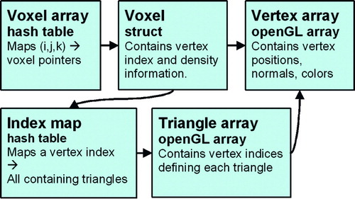
Additional data structures map each voxel to its corresponding vertex index, and each vertex index to the set of triangles that contain it. This allows rapid access to graphic rendering elements (vertices and triangles) given a modified bone voxel, which is critical for shading vertices based on voxel density and for re-triangulation when voxels are removed (see Bone removal section below). Figure 12 summarizes the relevant data structures.

Figure 12. A summary of the structures connecting our volumetric (haptic rendering) and surface (graphic rendering) data. When a voxel is removed or modified, the corresponding vertices and triangles can be accessed from the (i, j, k) voxel index in approximately constant time.

Haptic rendering

Virtual instruments are controlled using a SensAble Phantom [25] haptic device, which provides three-degree-of-freedom force-feedback and six-degree-of-freedom input.

Each of the bone modification tool models is discretized into a voxel grid (typically at a finer resolution than the bone grid), and a preprocessing step computes an occupancy map for the tool's voxel array. At each iteration of our haptic rendering loop, each of the volume samples in each active tool is checked for intersection with the bone volume. This operation can be performed rapidly (in constant time) using the hash table described above. Each sample point that is found to lie inside an occupied bone voxel generates a unit-length contribution to the overall haptic force vector that tends to push this sample point toward the tool center. With adequate stiffness, the tool center is always outside the bone volume (see Figure 13). For tools with an ill-defined center, the force vector generated by an immersed voxel is directed along the inward-pointing surface normal at the nearest surface point.

Figure 13. Our approach to haptic feedback. Red points are volume samples within the tool, blue points are volume samples within the bone. The full volume of the drill is sampled, and each point that is found to be immersed in the bone volume (shown in purple) contributes a vector to the overall force that points toward the center of the tool and is of unit length. [Color version available online.]

The overall force vector generated by our approach is thus oriented along a vector that is the sum of the “contributions” from individual volume sample points. The magnitude of this force is computed based on the number of sample points found to be immersed in the bone volume, which approximates the tool's penetration depth.

Bone removal

Each bone voxel is associated with a density value, initially derived from the original image data. Each time a tool sample is found to be in contact with a bone voxel, the density of that bone voxel is decreased. When a voxel reaches zero density, it is removed from the voxel array.

To maintain consistency between the graphic and haptic rendering systems, it is necessary to then re-tessellate the area around the removed bone. Consequently, bone voxels are queued by our haptic rendering thread as they are removed, and the graphic rendering thread retessellates the region around each voxel pulled from this queue. That is, for each removed voxel, the rendering thread checks whether any of the removed voxel's neighbors were previously internal but are now on the bone surface. Specifically, for each removed voxel v, we perform the following steps:

for each voxel v′ that is adjacent to v

 if v′ is on the bone surface

  if a vertex has not already been

  created to represent v′

   create a vertex representing v′

   compute the surface gradient at v′

  queue v′ for triangle creation

for each queued voxel v′

  generate triangles adjacent to v′

  (see below)

Once again, a voxel that is “on the bone surface” has a non-zero bone density and has at least one neighbor that has zero bone density. When all local voxels have been tested for visibility (i.e., when the first loop is complete in the above pseudocode), all new vertices are fed to a triangle generation routine. This routine finds new triangles that can be constructed from new vertices and their neighbors and orients those triangles to match the vertices' surface normals (defined using the voxel density gradient).

Additional tools

Our system also provides a planar cut tool (see Figure 14), used to introduce large divisions in the bone model. This tool does not generate haptic feedback and is not intended to simulate a physical tool. Rather, it addresses the need of instructors to make rapid cuts for the creation of training scenarios and for accelerated access to specific anatomy. The bone-removal function associated with this tool is implemented by discretizing the planar area – controlled in six degrees of freedom using the haptic device – into voxel-sized sample areas, and tracing a ray a small distance from each sample along the normal to the plane. This is similar to the approach used in reference 11 for haptic rendering, but no haptic feedback is generated. Each ray is given infinite “drilling power”, i.e., any voxels through which each ray passes are immediately removed. The distance traced along each ray is controlled by the user. This allows the user to remove a planar or box-shaped region of bone density, demonstrated in Figure 14b. In general, this approach will often generate isolated fragments of bone that the user wishes to move or delete; the processing of independent fragments is discussed later in this section (see Discontinuity detection).

Figure 14. The use of the cut-plane tool and the independent manipulation of discontinuous bone regions. (a) The cut-plane tool is used to geometrically specify a set of voxels to remove. (b) The volume after voxel removal. (c) The flood-filling thread has recognized the discontinuity, and the bone segments can now be manipulated independently. [Color version available online.]

An additional set of tools allows the user to manipulate rigid models that can be affixed to bone objects. This is particularly relevant for the target craniofacial procedures, which center around rigidly affixing metal plates to the patient's anatomy. We thus provide models of several distractors and/or Synthes bone plates; it is straightforward to add additional models to the system. The inclusion of these plate models allows users to plan and rehearse plate-insertion operations interactively, using industry-standard plates.

For each plate model, a set of sample points is generated by sampling 100 vertices of each model and extruding them slightly along their normals (because these models tend to be very thin relative to our voxel dimensions) (Figure 15a). Haptic feedback is generated using these sample points. In this case, since a very large area of the tool is often in contact with the bone, we elected to use the ray-tracing approach to haptic feedback generation presented in reference 11. This approach allows reasonable haptic feedback with fewer samples than the volumetric approach we use for our cutting tools. Since there is no well-defined tool center toward which we can trace rays for penetration calculation, rays are traced along the model's surface normal at each sample point. At any time, the user can rigidly affix a plate tool to a bone object with which it is in contact (Figure 15b–d). Future work will include a more sophisticated simulation of the bone-screw insertion process.

Figure 15. The modeling and attachment of rigid bone plates. (a) The surface of a bone plate after sampling and extrusion. (b) A bone surface before modification. (c) The same bone surface after drilling, distraction, and plate attachment. (d) The same bone surface after drilling, distraction, and distractor insertion. [Color version available online.]

Discontinuity detection

Introducing fractures in the bone model is a critical component of the target procedures. Our system thus needs to efficiently detect fractures that the user creates with the bone modification tools, then allow independent rigid transformations to be applied to the isolated bone segments.

In our environment, a background thread performs a repeated flood-filling operation on each bone structure. At each iteration of this thread, a random voxel is selected as a seed point for each bone object, and flood-filling proceeds through all voxel neighbors that currently contain bone density. Each voxel maintains a flag indicating whether or not it has been reached by the flood-filling operation; at the end of a filling pass, all un-marked voxels (which must have become separated from the seed point) are collected and moved into a new bone object, along with their corresponding data in the vertex and triangle arrays. Figure 16 summarizes this operation and provides an example.

Figure 16. Discontinuity detection by flood-filling. The seed voxel is highlighted in red, and the shaded (blue) voxels were reached by a flood-filling operation beginning at the seed voxel. These voxels thus continue to be part of the same bone object as the seed voxel, while the unshaded voxels on the right have become disconnected and thus are used to create a new bone object. In a subsequent pass through the flood-filling algorithm, a third bone object would be created, because the unfilled voxels are further fragmented. [Color version available online.]

Figures 14b and 14c display a bone object that has been cut and the subsequent independent movement of the two resulting structures. Here – for demonstration – the cut-plane tool is used to create the fracture; during simulated procedures, most fractures will likely be created by the drilling/sawing tools.

System description

The software described here was written in C + +and runs on a Windows-based PC. The planning tool runs on a 1-GHz desktop, and the haptic simulation environment runs on a dual-1.5-GHz workstation, using a SensAble Phantom Omni (SensAble Technologies, Woburn, MA) for haptic interaction.

Conclusion and future work

Initial feedback from craniofacial surgeons suggests that our environment provides a productive mechanism for visually exploring distraction procedures, and that the distraction paths generated by our system are appropriate for intraoperative use. Future work will focus on the automatic exporting of this distraction plan in a manner that will enable a manufacturer to produce the custom distractor, possibly including pre-bending of the distraction apparatus and automatic marking of individual steps along the distraction vector.

Additional work will focus on further development of our haptic simulation environment, to build a more formal training environment for new surgeons and to allow experienced surgeons to explore more difficult procedure components (e.g., the formation of the distraction apparatus) in more detail. We also hope to integrate our simulation environment with previous work on predictive modeling of facial appearance, to allow users to explore the probable outcome given a particular bone configuration, distraction path, and surgical approach. Furthermore, we hope to apply our simulation techniques to other surgical procedures with similar physical requirements; initial work on the application of our simulator to temporal bone surgery can be found in reference 26.

Acknowledgments

The authors would like to thank the AO Foundation, Intel Corporation, the NDSEG fellowship program, NIH LM07295, and CBYON systems for their generous support of this work.

References

- Ellis E, Moos K F, el-Attar A. Ten years of mandibular fractures: an analysis of 2,137 cases. Oral Surg Oral Med Oral Pathol 1985; 59(2)120–123
- State A, Livingston M A, Hirota G, Garrett W F, Whitton M C, Fuchs H, Pisano E D. Technologies for augmented reality systems: realizing ultrasound-guided needle biopsies. Proceedings of SIGGRAPH ‘96 1996; 439–446
- Merril G, Raju R, Merril J. Changing the focus of surgical training. VR World 1995; 3(2)56–58; 60–61
- Ziegler R, Fischer G, Muller W, Gobel M. Virtual reality arthroscopy training simulator. Computers in Biology and Medicine 1995; 25(2)193–203
- Wagner C, Schill M, Manner R. Interocular surgery on a virtual eye. Communications of the ACM 2002; 45: 45–49
- Scharver C, Evenhouse R, Johnson A, Leigh J. Designing cranial implants in a haptic augmented reality environment. Communications of the ACM 2004; 47(8)32–38
- Delingette H, Subsol G, Cotin S, Pignon J. Virtual reality and the simulation of craniofacial surgery. Proceedings of Interface to Real and Virtual Worlds. NanterreFrance 1994
- Keeve E, Girod S, Kikinis R, Girod B. Deformable modeling of facial tissue for craniofacial surgery simulation. Comput Aided Surg 1998; 3: 228–238
- Teschner M. Direct computation of soft-tissue deformation in craniofacial surgery simulation. 2001, Ph.D. thesis. Department of Engineering, Universität Erlangen-Nürnberg
- Teschner M, Girod S, Girod B. 3-D Simulation of craniofacial procedures. Proceedings of Medicine Meets Virtual Reality 2001, J D Westwood, H M Hoffman, G T Mogel, D Stredney. IOS Press, Amsterdam 2001
- Petersik A, Pflesser B, Tiede U, Höhn K H, Leuwer R. Haptic volume interaction with anatomic models at sub-voxel resolution. Proceedings of 10th Symposium on Haptic Interfaces for Virtual Environment and Teleoperator Systems (Haptics 2002), Orlando, FL, March, 2002; 66–72
- Agus M, Giachetti A, Gobbetti E, Zanetti G, Zorcolo A. A multiprocessor decoupled system for the simulation of temporal bone surgery. Computing and Visualization in Science 2002; 5(1)35–43
- Bryan J, Stredney D, Wiet G, Sessanna D. Virtual temporal bone dissection: A case study. Proceedings of IEEE Visualization 2001, T Ertl, et al, October, 2001; 497–500
- Pflesser B, Petersik A, Tiede U, Höhne K H, Leuwer R. Volume cutting for virtual petrous bone surgery. Comput Aided Surg 2002; 7(2)74–83
- Gibson S, Samosky J, Mor A (1997) Simulating arthroscopic knee surgery using volumetric object representations, real-time volume rendering and haptic feedback. Proceedings of First Joint Conference on Computer Vision, Virtual Reality and Robotics in Medicine and Medical Robotics and Computer-Assisted Surgery (CVRMed-MRCAS’97), GrenobleFrance, March, 1997, J Troccaz, E Grimson, R Mösges. 369–378, Lecture Notes in Computer Science Vol 1205. Berlin: Springer;
- Morris D, Girod S, Barbagli F, Salisbury K (2005) An interactive simulation environment for craniofacial surgical procedures. Proceedings of Medicine Meets Virtual Reality (MMVR), Long Beach, CA, January, 2005. IOS Press, Amsterdam
- Rohlfing T, Maurer C R, Jr. (2001) Intensity-based non-rigid registration using adaptive multilevel free-form deformation with an incompressibility constraint. Proceedings of 4th International Conference on Medical Image Computing and Computer-Assisted Intervention (MICCAI 2001), UtrechtThe Netherlands, October, 2001, W J Niessen, M Viergever. 111–119, Lecture Notes in Computer Science Vol 2208. Berlin: Springer;
- Liu Y, Collins R, Rothfus W E. Robust midsagittal plane extraction from normal and pathological 3D neuroradiology images. IEEE Trans Med Imaging 2001; 20(3)175–192
- Prima S, Ourselin S, Ayache N. Computation of the mid-sagittal plane in 3-D brain images. IEEE Trans Med Imaging 2002; 21(2)122–138
- Nienhuys H, van der Stappen A F. A Delaunay approach to interactive cutting in triangulated surfaces. Proceedings of 5th International Workshop on the Algorithmic Foundations of Robotics, NiceFrance, December, 2002
- Foley J D, van Dam A, Feiner S K, Hughes J F. Computer graphics: principles and practice. Second edition. Addison Wesley;. 1987
- Lorensen W, Cline H. Marching Cubes: A high resolution 3D surface construction algorithm. Computer Graphics 1987; 21(4)163–169
- van den Bergen G. Efficient collision detection of complex deformable models using AABB trees. J Graphics Tools 1997; 2(4)1–13
- Bouvier D J. Double-Time Cubes: A fast 3D surface construction algorithm for volume visualization. Proceedings of First International Conference on Imaging Science, Systems, and Technology, Las Vegas, NV, June 30–July 3, 1997
- Massie T H. Salisbury JK: The PHANTOM haptic interface: A device for probing virtual objects. Proceedings of Symposium on Haptic Interfaces for Virtual Environments, Chicago, IL, November, 1994
- Morris D, Sewell C, Blevins N, Barbagli F, Salisbury K (2004) A collaborative virtual environment for the simulation of temporal bone surgery. Proceedings of 7th International Conference on Medical Image Computing and Computer-Assisted Intervention (MICCAI 2004), Saint-MaloFrance, September, 2004, C Barillot, D R Haynor, P Hellier. 319–327, Lecture Notes in Computer Science Vol 3217. Berlin: Springer;