Bone enhancement filtering: Application to sinus bone segmentation and simulation of pituitary surgery

Abstract

The simulation of pituitary gland surgery requires a precise classification of soft tissues, vessels and bones. Bone structures tend to be thin and have diffuse edges in CT data, and thus the common method of thresholding can produce incomplete segmentations. In this paper, we present a novel multi-scale sheet enhancement measure and apply it to paranasal sinus bone segmentation. The measure uses local shape information obtained from an eigenvalue decomposition of the Hessian matrix. It attains a maximum in the middle of a sheet, and also provides local estimates of its width and orientation. These estimates are used to create a vector field orthogonal to bone boundaries, so that a flux maximizing flow algorithm can be applied to recover them. Hence, the sheetness measure has the essential properties to be incorporated into the computation of anatomical models for the simulation of pituitary surgery, enabling it to better account for the presence of sinus bones. We validate the approach quantitatively on synthetic examples, and provide comparisons with existing segmentation techniques on paranasal sinus CT data.

• Bone segmentation
• structure tensor
• Hessian matrix
• geometric flows
• CT
• multi-scale analysis
• validation

Introduction

Pituitary gland tumors represent the third most common primary intracranial tumors encountered in neurosurgical practice, with a reported annual incidence ranging from 1 to 14.7 per 100,000 persons. In the majority of cases, a surgical intervention is required. To reach the pituitary gland, a neurosurgeon typically enters through the nose and has to break thin paranasal sinus bones and remove soft tissues while avoiding nerves and blood vessels (Figure 1). This requires extensive practice and precise knowledge of the anatomy, the absence of which can have serious implications for the patient [3]. Currently, the only way to train a neurosurgery resident for such an operation is by multiple observations and by elementary maneuver attempts supervised by an expert neurosurgeon. As a result, for the past several years there has been an interest in building a surgical simulator to aid in such training. Existing surgical simulators generally involve a generic anatomical model elaborated on the basis of extensive human supervision, interacting with a fast but constitutively limited biomechanics engine. One goal of our research is to formulate a minimally supervised method for producing a set of patient-specific anatomical models, from MR and CT datasets, in a manner that can interact with a hierarchical finite-element-based biomechanics engine. To do so, we need a precise 3-dimensional (3D) partition of tissue classes into bone, air, vessel, nerve and soft tissue.

Figure 1. Anatomy of pituitary gland area (adapted from reference [1]) (left); and a schematic demonstrating endoscopic pituitary surgery (adapted from reference [2]) (right).

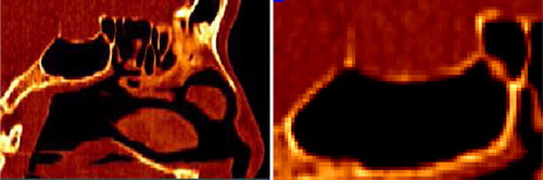
In this paper we focus on paranasal sinus bone enhancement and segmentation from CT data. The common methods for segmentation of bone in CT are based on thresholding followed by the use of image connectivity measures or manual editing, which is both tedious and prone to human error. At a coarse scale, segmentation by thresholding is quite good due to the 3-class nature of CT images and the known Hounsfield value range for bone. Air has almost no signal and bone has a much higher signal than surrounding tissues. However, thin bones can have holes and diffuse boundaries due to partial volume effects and noise in CT datasets, as illustrated in Figure 2. Thus, for such thin bones, a simple thresholding procedure gives unsatisfactory results.

Figure 2. Sagittal slice of a CT dataset in the region of interest for pituitary gland surgery (see Figure 1). In the image, black corresponds to air, gray to soft tissue, and white to bone. Note the low intensity values and holes in the bone structure at right. This is an important bone the neurosurgeon needs to break in order to reach the pituitary gland.

We introduce a novel algorithm for bone enhancement filtering and segmentation. Whereas our approach is motivated by the problem of paranasal sinus bone segmentation, it can in fact be used to enhance and segment any sheet-like structure, since it is based on a general multi-scale second-order local shape operator. We exploit the eigenvalue decomposition of the Hessian matrix, which is known to give valuable local information by which to discriminate between blob-like, tube-like and sheet-like iso-intensity level sets in the image [4–8]. We propose a sheetness measure that can be used to drive an active surface to segment bone. This is motivated in part by Frangi et al.'s tubular structure enhancement filtering measure [5] and Descoteaux et al.'s [4] multi-scale geometric flow. We illustrate the power of the approach with segmentation results in regions with holes and low Hounsfield values in CT data and compare these to results from reference [9] based on local structure extraction with the structure tensor. We also validate the approach quantitatively on synthetic data. To our knowledge, our method is the first flow-based approach for paranasal sinus bone segmentation.

The article is organized as follows. In the next section we review background material on the use of local 3D structure models for segmentation, as well as existing active contour algorithms for bone extraction. We then develop a sheetness measure and use it to drive a flux maximizing flow algorithm [10] for bone segmentation. In the subsequent section, we validate the approach on synthetic data and also provide comparative results against the structure tensor approach on a high-resolution CT dataset. The paper then concludes with a discussion.

Materials and methods

Using local 3D structure for filtering and segmentation

We begin by considering image filtering algorithms which use the structure tensor 𝒯 and the Hessian matrix ℋ as shape descriptors. For a 3D image image ℐ, these are defined as

In both cases, an eigenvalue analysis is performed to extract the local behavior of iso-intensity level sets in the image. Many methods have been developed for blood vessel segmentation using these models [4–8], and we review only a selection of representative techniques here.

Modeling sheet-like structures with the tensor descriptor

As mentioned previously, a common method for bone segmentation in CT data is to use simple thresholding, an approach that can fail on thin bone structures. Westin et al. [9], [11] have recently introduced an adaptive thresholding approach using the structure tensor to segment thin bones around the eye socket and in the paranasal sinus area. The idea is to evaluate the positive semi-definite structure tensor 𝒯 at every voxel of the data and determine the degree to which its shape resembles a line, a plane or a sphere. Letting λ₁, λ₂, λ₃ (0 ≤ λ₁ ≤ λ₂ ≤ λ₃) be the eigenvalues of the structure tensor, and e₁, e₂, e₃ the corresponding eigenvector, the interest is when the tensor can be approximated by a plane. In that case, tensor τ has rank 1 which means that the two smallest eigenvalues are null, i.e., λ₁ = λ₂ = 0 and λ₃ > >0 (see reference [9] for more details). The authors then describe a planar measure,such that, in theory, it has a value of 1 for plane structures and 0 for others. This measure is used to adaptively threshold the input dataset ℐ. The threshold at each voxel x is then defined aswhere t₀ is a global threshold manually selected depending on the dynamics of the input image and α is a weight factor on the planar measure.

In the results section, we demonstrate several properties of this approach. In particular, 𝒯 is positive semi-definite, which means that all its eigenvalues are positive, i.e., λ₁, λ₂ λ₃ > 0. Moreover, since the tensor is based on first-order variation, the c_plane measure is strong at boundaries (where the gradient is strong) and weak inside the bone structure. For our application, we seek a measure that is high at the center of the structure with a fall off at boundaries where, a priori, our confidence in a voxel being strictly bone or strictly soft tissue is weak. Such a confidence index can guide the subsequent surface and volume meshing of bone tissue relevant to the simulation of pituitary surgery. We explore the properties of the Hessian shape operator to define such a measure.

Modeling sheet-like structures using the Hessian operator

The Hessian matrix encodes important shape information. Whereas the structure tensor models the first-order changes in intensity, the Hessian examines second-order variations of the data. An eigenvalue decomposition measures the maximum changes in the normal vector (gradient vector) of the underlying intensity iso-surface in a small neighborhood. (Details on the mathematical justification between differential geometry of surfaces and the Hessian operator can be found in reference [13].) Hence, it can differentiate between tube-like, sheet-like and blob-like structures. The classification of Table I was first explored by Sato et al. [8], and Lorenz et al. [7] separately. In reference [5], Frangi defines three ratios using tube-like properties of the eigenvalues of Table I to separate blood vessels from other structures,

Table I.  Local structure classification based on the Hessian matrix, assuming | λ₁ | ≤ | λ₂ | ≤ | λ₃ | [7], [8].

Eigenvalue conditions	Local structure	Examples
λ1 ≈ λ2 ≈ 0, λ3 > >0	sheet-like	bone, skin
λ1 ≈ 0, λ2 ≈ λ3 > >0	tube-like	vessels, nerves
λ1 ≈ λ2 ≈ λ3 > >0	blob-like	nodule
lambda1 ≈ λ2 ≈ λ3 ≈ 0	noise-like	background, noise

From Table I, it can be seen that R_B is non-zero only for blob-like and noisy structures. The R_A ratio differentiates sheet-like from tube-like structures. Finally, R_noise, the Frobenius norm, is used to ensure that random noise effects are suppressed from the response. For a particular scale σ, the intensity image is convolved with derivatives of γ-parameterized Gaussian kernels [12] with standard deviation σ to compute the Hessian matrix. A vesselness response function V(σ) is then computed. (The vesselness expression is given for the case of a dark tubular structure on a brighter background (as in proton density MRI). In the case of angiographic data, the signs in condition 1 must be changed, i.e., V(σ)=0 if λ₂ > 0 or λ₃ > 0.):

Due to the multi-scale approach, the vesselness measure is designed to be maximum when computed at the scale corresponding to the radius of the tubular objects. The vessel index is thus maximum nearby the vessel center and is zero outside. In reference [4], a vesselness measure is used to find putative centerlines of tubular structures, along with their estimated radii, and is then distributed to create a vector field which is orthogonal to vessel boundaries, so that the flux maximizing flow algorithm of reference [10] can be applied to recover them. This method can recover low-contrast and thin vessels from standard anatomical proton density weighted datasets.

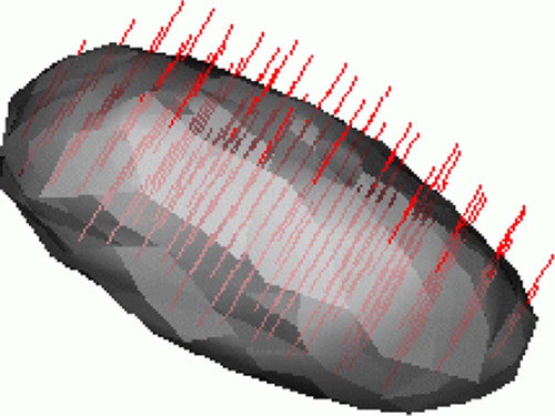
Motivated by these approaches, we propose a multi-scale sheetness measure that enhances bone structures, and then use it to drive a deformable surface that stops at bone boundaries. At every voxel we determine whether the underlying iso-intensity surface behaves like a sheet. When it does, we know that the eigenvectors corresponding to the null eigenvalues span the plane of the sheet, and that the other eigenvector is perpendicular to it (see Figure 3).

Figure 3. Distribution surface illustration: an ellipsoid with one short semi-minor axis corresponding to the detected scale of the sheet-like structure and two equal semi-major axes that we choose to be twice the semi-minor axis. The eigenvectors of the Hessian matrix corresponding to non-zero eigenvalues are shown in red. They are locally perpendicular to the sheet-like structure.

We define two new ratios, R_sheet and R_blob, and re-use R_noise, defined in Equation 3, to differentiate sheet-like structures from others:Their theoretical behavior is described in Table II. Then, following Frangi et al. [5], we define the sheetness measure, M, as the maximum response over all scales σ at which the derivatives of the Hessian are computed. Specifically,where Σ is a finite set of scales chosen by the user in the range of smallest to thickest possible bone structures (0.5 ≤ σ ≤ 3.0) in the data. The parameters α, β, c are set to 0.5, 0.5 and half the maximum Frobenius norm(R_noise), respectively, as suggested in references [4], [5].

Table II.  Theoretical properties of the ratios defined to construct the sheetness measure.

Ratios	Sheet	Tube	Blob	Noise
Rsheet = | λ2 |/| λ3 |	0	1	1	undefined
Rblob = | (2 | λ3 | − | λ2 | − | λ1 |) |/| λ3 |	2	1	0	undefined
	λ3	√2λ3	√3λ3	0

Each term of the equation has a function that depends on the characteristics of Table II. To avoid division by a null λ₃ in the case of noise, the undefined can be set to obtain the desired behavior. Breaking down the terms of Equation 6, we have

1. is a sheet enhancement term, where the maximum occurs for sheet-like structures and the minimum for others. We set undefined to 1.

2. is a blob and noise elimination term since it is zero for both. Moreover, the term is high for a sheet and low for a tube. We set undefined to zero.

3. is a background or noise reduction term. R_noise is known as the Frobenius norm and is high only in the presence of structure.

Note that we do not define a tube elimination term, as the curved ends of bone structures have a behavior that is both tube-like and sheet-like. Thus, the sheetness measure is designed to be maximum for sheet-like voxels, lower for tube-like regions, and zero for other structures. The advantage of this approach is that after the sheetness computation, we have a confidence sheet-like score at each voxel and in addition, for high score locations, the scale estimate of the radius of the sheet as well as the normal vector to the plane.

A geometric flow for segmenting bone structures

The deformable model is commonly used for segmentation in many computer vision applications and the corresponding literature is very rich, motivated in large part by the classical parametric snakes introduced by Kass et al. [15]. These models have also been extended to handle changes in topology due to the splitting and merging of contours [16]. However, there have been a few deformable model methods proposed for bone segmentation that are quite different from our approach because they are suited for 2D images from different modalities and different bones ([17–19]). In reference [17], the segmentation of carpal bones of the hand in CT images is faced with similar challenges as in our sinus bone CT dataset. A skeletally coupled curve evolution framework is proposed that combines probabilistic growth with local and global competition. Promising results are shown on 2D images with gaps and diffuse edges. However, the method is based on skeletal points that would be difficult to determine in bone structures that are only one or two voxels wide, such as those in the paranasal sinuses.

In our application, we propose to use the bone enhancement measure of Equation 6 to drive a 3D surface evolution. We construct a vector field that is both large in magnitude and orthogonal to bone structures. The key idea is to distribute the sheetness measure, which is concentrated on the center sheet, to the bone boundaries implied by the local scale and direction estimates from the multi-scale sheetness measure of Equation 6. At each voxel where the sheetness index is high, we consider a disc or flat ellipsoid with its two semi-minor axes aligned with the estimated plane orientation and its semi-major axis equal to the approximated radius. The sheetness measure is then distributed over every voxel on the boundary of the disc. We define the addition of the extensions carried out independently at all voxels to be the ϕ distribution. An extended vector field is now defined as the product of the normalized gradient of the original image with the above ϕ distribution,The extended vector field of Equation 7 explicitly models the scale at which bone boundaries occur, due to the multi-scale nature of the sheetness measure M (Equation 6) as well as the expected gradient in the direction normal to bone boundaries. Thus, it is an ideal candidate for the static vector field in the flux maximizing geometric flow of Vasilevsky et al. [10], . The flow evolves the surface S in time t to converge to the zero-crossing of the speed term, . The surface evolution equation works out to beHere, κ_ℐ is the Euclidean mean curvature of the iso-intensity level set of the image. Note that this is a hyperbolic partial differential equation, since all terms depend solely on the vector field and not on the evolving surface. We now enumerate several properties of this geometric flow.

1. The first term acts like a doublet. ∇ϕ has a zero-crossing at bone boundaries and ∇ ℐ does not change sign. Hence, when the evolving surface overshoots the boundary slightly, this term acts to push it back toward the boundary. Such doublet terms have also shown to be beneficial in earlier geometric flows for segmentation [20–22].

2. The second term behaves like a geometric heat equation since κ_ℐ is the mean curvature of the iso-intensity level set of the original intensity image. This equation has been extensively studied in the mathematics literature and has been shown to have remarkable anisotropic smoothing properties [23], [24]. It is also the basis for several nonlinear geometric scale-spaces, such as those studied in references [25], [26].

3. Combining both terms, it is clear that the flow cannot leak in regions outside vessels since both ϕ and ∇ϕ are zero there. Hence, when seeds are placed at locations where the sheetness measure M is high, the flow given by Equation 8 will evolve toward the closest zero level set of the divergence of the vector field . This is clearly illustrated in the synthetic segmentation examples of Figure 4.

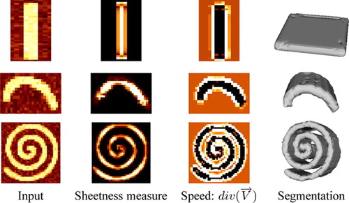
Figure 4. Experiment on synthetic objects. Slices of the input volumes, the sheetness measure, the speed term, and a surface rendering of the segmentation.

Implementation details

Below we review some of the details of the implementation of the multi-scale geometric flow (Equation 8), which is based on level set methods [27]. The flow is topologically adaptive due to its implementation with levelset, is computationally efficient, and requires minimal user interaction. We refer the reader to reference [4] for further details on the vector field construction and implementation of the flux maximizing surface evolution.

1. The ϕ distribution is carried out from voxels at bone structure center sheets, since at such locations one has strong confidence in the scale and orientation estimate from sheetness measure. This is done using the following procedure:We use a sheetness threshold of 0.01 and a percentile of 0.75 and local_max is the maximum sheetness response in a 3 × 3 × 3 neighborhood of the voxel. The voxels inside the ellipsoidal regions give the seeds used to initialize the geometric flow. These parameters give good and stable vessel extractions over all three image modalities tested: angiography, gadolinium and PD.

2. The derivatives in the doublet term are computed using central differences for ∇ϕ and a second-order essentially non-oscillatory (ENO) scheme for the normalized gradient of the input image [28]. This is essentially because ϕ is by construction relatively smooth, since it is constructed by superposition. On the other hand, the gradient of the original intensity image can be sharp and is better captured by an ENO method.

3. κ_ℐ, the mean curvature of each intensity iso-surface is computed using a 3-neighbor central difference scheme for all derivatives:

4. A first-order in time discretized form of the levelset version of the evolution equation is given bywhere , Ψ is the embedding hypersurface and Δt is the step size. This is now a standard numerical approach for solving partial differential equations of this type since it allows topological changes to occur without any additional computational complexity and can be made efficient using a narrow band implementation.

5. The evolving surface S is obtained as the zero level set of the Ψ function. The numerical derivatives used to estimate ‖ ∇ Ψ ‖ must be computed with up-winding in the proper direction, as described in reference [27].

Experimental results

Quantitative validation on synthetic objects

In order to validate the extension of the sheetness measure to boundaries and evaluate the effectiveness of the speed term driving the geometric flow, we constructed several binary synthetic objects of varying widths and curvatures. Each volume was then smoothed using two iterations of mean curvature smoothing to simulate partial volume effects at their boundaries. Ground-truth surface points were obtained as the 0.5 crossings of each object, obtained by linear interpolation on the voxel grid. We then added white Gaussian noise to each voxel to simulate typical noise levels in a CT acquisition process (we used a 10% signal-to-noise ratio) and followed the steps detailed above to construct the sheetness measure, obtain the ϕ distribution, and then build the vector field , using the same parameters throughout. Empirical surface points were defined as the zero-crossings of the speed term in the geometric flow.

Figure 4 illustrates the various terms. We evaluated the accuracy of the zero-crossings of the speed term by computing the average and maximum Euclidean distance errors between each empirical surface voxel and its closest ground-truth surface voxel. This measure indicates the degree to which the segmented data explains the ground-truth data, but in terms of an average distance error. We also computed the ratio between classified voxels in the segmentation and bone voxels in the binary volume. This measure indicates the degree to which the ground-truth data is accounted for by the segmented data.

The results, shown in Table III, indicate that the average error is typically less than 0.3 voxels and that the agreement between the reconstructed and original volume is above 90%. We have determined empirically that the maximum errors occur at the two ends of each synthetic object, which is to be expected since mean curvature smoothing causes the most shrinkage there. Finally, note that we have run the experiments with signal-to-noise ratios of 20% and 5% without dramatically affecting the synthetic segmentations. The overall behavior is the same and is robust with reasonable noise level. This is mainly due to the smoothness level imposed by of the multiscale sheetness computation with convolutions of Gaussian derivatives.

Table III.  The agreement level between the ground truth boundary and and that obtained by the geometric flow.

Object	Average distance error (voxels)	Maximum error (voxels)	Ratio (%)
plate	0.22	1.00	95
rib	0.25	1.12	95
spiral	0.26	1.22	91

Bone enhancement and segmentation on CT data

We chose to compare our technique with two other approaches in the literature, Westin et al.'s adaptive thresholding method and simple thresholding. To perform this comparison, we cropped a 53 mm × 89 mm × 98 mm region of a CT dataset around the paranasal sinuses, resampled it to a 0.468 mm³ isotropic grid, and ran the segmentation methods.

We make two qualitative observations from the results, which are shown in Figure 5. First, we see that both the algorithm of Westin et al. [9] and our method work better than simple thresholding. Second, our method appears to better exploit tissue contiguity and connect more bone structure than Westin et al.'s approach. This is to be expected, since our geometric flow method is designed to connect sheet-like regions whereas the approach of Westin et al. remains a thresholding method, albeit one that accounts for local structure. We have chosen adaptive thresholding (c_plane) parameters which gave the best results, but it is clear that if incorporated in an deformable model framework (as the authors suggest) a better segmentation could be obtained.

Figure 5. Comparison between different segmentation methods. Our method connects most of the thin bone structure and reconstructs more bone than the approach in reference [1] and thresholding.

4 Discussion

We have presented a multi-scale bone enhancement measure that can be used to drive a geometric flow to segment sheet-like structures. The key contribution is the introduction of a sheetness measure M based on the properties of the multi-scale Hessian shape operator. We have validated our approach quantitatively on synthetic examples and have compared existing segmentation techniques on paranasal sinuses in a CT dataset. The measure indicates confidence in the presence of bones and, for voxels with high values, their local scale and direction. We should point out that the same method can be applied to segment other sheet-like structures in different modalities, e.g., it can be used for skull segmentation in CT or MRI data.

In our experiments with the approach of Westin et al. [9] we have found that the structure tensor picks out the direction of maximum change in intensity, but the c_plane measure is strong mostly at boundaries and thus tends to thicken the edges. This can be seen in the tensor norm response in Figure 5. Our method has the advantage of extracting locations at the center of bone structures, where the underlying iso-intensity level set behaves locally like a plane.

The sheetness measure combined with a flow designed to evolve and stop at boundaries is able to propagate along low sheetness regions. Used on its own, the sheetness measure has suitable characteristics to be incorporated into a surgical simulator for pituitary intervention. The measure is high on the center plane and decreases towards the boundaries, where there is less certainty in the tissue classification of a voxel. Hence, it can allow a surface mesh model to account for uncertainty in determining triangulated bone boundaries, to better model sinus bones in the simulation. For surgical simulation, it might, in fact, be more useful to have a confidence measure for all voxels than a binary segmentation of bones.

One can imagine combining the respective strengths of the structure tensor and Hessian operators into a hybrid operator. Krissian et al. [14] do so with a new positive semi-definite and scale-invariant descriptor to infer the local shape behavior of the aorta from low-quality ultrasound images. Although this is a different problem and is concerned with a different modality, the underlying model uses similar ideas. In particular, it is also based on a multi-scale eigenvalue decomposition at each voxel to obtain the local orientation and the cross-sectional plane of the aorta. However, the proposed hybrid operator is essentially a generalization of the structure tensor, and thus has certain limitations. The main difficulty, for our application, is the stronger response of operators involving the structure tensor at bone boundaries. Another problem is the positive semi-definiteness of such operators. Having all eigenvalues with the same sign is actually a disadvantage in our application, because one cannot differentiate between grey-to-white and white-to-grey change of intensity in the signal. In the paranasal sinus area, where bone structures are thin and very close to one another, the response from the shape operator must be able to make this distinction. Hence, in this paper, we only use the Hessian operator to perform the eigenvalue decomposition and define the sheetness measure M of Equation 6.

In future work we plan to use both the bone segmentation as well as the sheetness, vesselness and other tissue classification cues from the CT and corresponding MRI data in a global class competition levelset framework for segmentation. This would provide a complete characterization of the tissues in the pituitary gland region, which could then employed in a virtual endoscopic surgery simulator.

Acknowledgments

We would like to thank the JSPS and NSERC summer program in Japan for funding this research. A special thank you to Alexandre Thinnes for valuable input in this work.

References

- Jastrow H., http://www.uni-mainz.de/FB/Medizin/Anatomie/workshop/VH/female/Filme/Filme.html
- Jho H. D., http://drjho.com/pituitary_surgery.htm
- Ciric I., Ragin A., Baumgartner C., Pierce D. Complications of transsphenoidal surgery: Results of a national survey, review of the literature, and personal experience. Neurosurgery 1997; 40(2)225–236
- Descoteaux M., Collins L., Siddiqi K. (2004) A multi-scale geometric flow for segmenting vasculature in MRI. Proceedings of the 7th International Conference on Medical Image Computing and Computer-Assisted Intervention (MICCAI 2004), Saint-MaloFrance, September, 2004, C. Barillot, D. R. Haynor, P. Hellier. Springer, Berlin, 500–507, Part I. Lecture Notes in Computer Science 3216
- Frangi A., Niessen W., Vincken K. L., Viergever M. A. (1998) Multiscale vessel enhancement filtering. Proceedings of the First International Conference on Medical Image Computing and Computer-Assisted Intervention (MICCAI ′98), Cambridge, MA, October, 1998, W. M. Wells, A. Colchester, S. Delp. Springer, Berlin, 130–137, Lecture Notes in Computer Science 1496
- Krissian K., Malandain G., Ayache N. Model-based detection of tubular structures in 3D images. Computer Vision and Image Understanding 2000; 80(2)130–171
- Lorenz C., Carlsen I., Buzug T., Fassnacht C., Weese J. (1997) Multi-scale line segmentation with automatic estimation of width, contrast and tangential direction in 2D and 3D medical images. Proceedings of First Joint Conference on Computer Vision, Virtual Reality and Robotics in Medicine and Medical Robotics and Computer-Assisted Surgery (CVRMED-MRCAS ′97), GrenobleFrance, March, 1997, J. Troccaz, E. Grimson, R. Mosges. Springer, Berlin, 233–242, Lecture Notes in Computer Science 1205
- Sato Y., Nakajima S., Atsumi H., Koller H., Gerig G., Yoshida Y., Kikinis R. 3D multi-scale line filter for segmentation and visualization of curvilinear structures in medical images. Med Image Anal 1998; 2(2)143–168
- Westin C-F, Bhalerao A., Knutsson H., Kikinis K. Using local 3D structure for segmentation of bone from computer tomography images. Proceedings of IEEE Computer Society Conference on Computer Vision and Pattern Recognition (CVPR ′97), San Juan, Puerto Rico, June, 1997; 794–800
- Vasilevskiy A., Siddiqi K. Flux maximizing geometric flows. IEEE Trans Pattern Anal Machine Intell 2002; 24(12)1–14
- Westin C-F, Warfield S., Bhalerao B., Mui L., Richolt J., Kikinis K. (1998) Tensor controlled local structure enhancement of CT images for bone segmentation. Proceedings of the First International Conference on Medical Image Computing and Computer-Assisted Intervention (MICCAI ′98), Cambridge, MA, October, 1998, W. M. Wells, A. Colchester, S. Delp. Springer, Berlin, 1205–1212, Lecture Notes in Computer Science 1496
- Lindeberg T. Edge detection and ridge detection with automatic scale selection. Int J Comput Vision 1998; 30(2)77–116
- Descoteaux M. A multi-scale geometric flow for segmenting vasculature in MRI: theory and validation. School of Computer Science, McGill University. June, 2004, MSc thesis
- Krissian K., Ellsmere J., Vosburgh K., Kikinis R., Westin C. F. Multiscale segmentation of the aorta in 3D ultrasound images. Proceedings of the Annual International Conference of the IEEE Engineering in Medicine and Biology Society, CancunMexico, September, 2003; 638–641
- Kass M., Witkin A., Terzopoulos D. Snakes: Active contour models. Int J Comput Vision 1987; 1: 321–331
- McInerney T., Terzopoulos D. T-snakes: Topology adaptive snakes. Med Image Anal 2000; 4: 73–91
- Sebastian T. B., Tek H., Crisco J. J., Kimia B. B. Segmentation of carpal bones from 3D CT images using skeletally coupled deformable models. Proceedings of the First International Conference on Medical Image Computing and Computer-Assisted Intervention (MICCAI ′98), Cambridge, MA, October, W. M. Wells, A. Colchester, S. Delp. Springer, Berlin 1998; 1184–1194, Lecture Notes in Computer Science 1496
- Ballerini L., Bocchi L. Bone segmentation using multiple communicating snakes. 2003; 1621–1628, SPIE Medical Imaging: Image Processing. SPIE volume 5032
- Lorigo L. M., Faugeras O. D., Grimson W. E.L., Keriven R., Kikinis R. (1998) Segmentation of bone in clinical knee MRI using texture-based geodesic active contours. Proceedings of the First International Conference on Medical Image Computing and Computer-Assisted Intervention (MICCAI ′98), Cambridge, MA, October, 1998, W. M. Wells, A. Colchester, S. Delp. Springer, Berlin, 1195–1204, Lecture Notes in Computer Science 1496
- Kichenassamy S., Kumar A., Olver P., Tannenbaum A., Yezzi A. Gradient flows and geometric active contour models. Proceedings of the 5th International Conference on Computer Vision, Cambridge, MA, May, 1995; 810–815
- Caselles V., Kimmel R., Sapiro G. Geodesic active contours. Proceedings of the 5th International Conference on Computer Vision, Cambridge, MA, May, 1995; 694–699
- Siddiqi K., Lauziere Y. B., Tannenbaum A., Zucker S. W. Area and length minimizing flows for shape segmentation. IEEE Trans Image Processing 1998; 7(3)433–443
- Gage M., Hamilton R. The heat equation shrinking convex plane curves. J Differential Geometry 1986; 23: 69–96
- Grayson M. The heat equation shrinks embedded plane curves to round points. J Differential Geometry 1987; 26: 285–314
- Alvarez L., Guichard F., Lions P. L., Morel J. M. Axiomes et equations fondamentales du traitement d'images. C R Acad Sci Paris 1992; 315: 135–138
- Kimia B. B., Tannenbaum A., Zucker S. W. Shape, shocks, and deformations I: The components of two-dimensional shape and the reaction-diffusion space. Int J Comput Vision 1995; 15: 189–224
- Osher S. J., Sethian J. A. Fronts propagating with curvature dependent speed: Algorithms based on Hamilton-Jacobi formulations. J Computational Physics 1988; 79: 12–49
- Osher S., Shu C. W. High-order essentially non-oscillatory schemes for Hamilton-Jacobi equations. SIAM J Numerical Anal 1991; 28: 907–922