Computerized planning of prostate cryosurgery with pullback operation

Abstract

This study is a part of an ongoing project to develop computerized tools for cryosurgery planning. Prostate cryosurgery is frequently performed as a two-stage process in which the first-stage targets are frozen with the cryoprobes at a greater insertion depth, while the second stage of freezing is performed after some cryoprobes are pulled back to new locations, this process being known as the pullback procedure. This paper proposes a method to generate computationally a preferred cryoprobe layout for the pullback operation, using a previously proposed bubble-packing method for cryosurgery planning. For this purpose, additional constraints are imposed to align packed bubbles along the same insertion path between the different stages, and to vary the number of bubbles at each stage. The method is demonstrated on 3D patient models from four individuals, using cryoprobes with a diameter of 1.5 mm and an active length of 15 mm. Results are verified with bioheat transfer simulations, and compared with the non-pullback operations using cryoprobes with longer (25 mm) active lengths. When compared with results of the non-pullback procedure, results with pullback suggest some improvement in freezing in the apex region of the prostate, with a slight increase in overall freezing damage to surrounding healthy tissues.

• Cryosurgery
• prostate
• pullback
• computerized planning
• bubble packing
• bioheat simulations

Introduction

Cryosurgery is the destruction of undesired biological tissue by freezing [1]. Minimally invasive cryosurgery is performed by means of cryoprobes, each having the shape of a long hypodermic needle with a sharp pointed tip. During the surgical operation, a cooling sink is created at the tip of the cryoprobe by the effect of either liquid nitrogen boiling or Joule-Thomson cooling (i.e., the cooling effect associated with a sudden change in pressure of a gas flowing through a nozzle), with the latter being more widely used in recent years. Prostate cryosurgery was the first minimally invasive cryosurgical procedure to pass from the experimental stage to a routine surgical treatment [2]. The minimally invasive approach created a new level of difficulty in surgery planning, in which a pre-defined 3D region of tissue must be treated with an array of cryoprobes while minimizing the damage to surrounding healthy tissue. Cryosurgical planning must consider not only the cooling probes, but also a heating device, known as the urethral warmer (the urethra extends nearly to the center of the prostate). The urethral warmer is embodied in a standard catheter, providing a close-to-core body temperature of 37°C along its outer surface. Use of the urethral warmer has been demonstrated to minimize post-cryosurgical complications associated with damage to the urethra [3].

The need to find an optimal cryoprobe layout is well documented, and several efforts to develop computerized means for planning have been reported in the literature [4–6]. While the order of significance of cryosurgical parameters to be optimized is still open to debate, the common clinical practice is based on the combination of geometrical considerations with the thermal history of the target region. Following this clinical approach, several methods for optimizing the best cryoprobe layout have been proposed [5–7]. However, these methods rely on a series of bioheat transfer simulations, a process which has proven to be very expensive computationally, and which cannot be fitted into a realistic clinical timeframe.

The shape of the frozen region is observed to be dependent on the cryoprobe layout and on the cooling capabilities of each cryoprobe. This observation led the present research group to adopt the “bubble-packing” method [8–10] for initial cryosurgery planning. Bubble packing is a physically based approach which evenly distributes a pre-defined number of elements in a given geometrical domain. Here, the domain is the prostate and the elements are the cryoprobes. While using the bubble-packing method as Phase I of planning, the so-called “force-field analogy” has been suggested as Phase II for planning refinement. The force-field analogy is an iterative method for distributing cryoprobes in the domain in order to match its boundary with a pre-specified isotherm [7]. The force-field analogy uses a sequence of bioheat transfer simulations, where the resulting temperature distribution of a specific layout applies “forces” to relocate cryoprobes before the following bioheat transfer simulation is executed. While the force-field method has proven to be robust, and is much less time-consuming than traditional gradient-descent methods [4–6], its advantages as a Phase II 3D planning tool were considered to be debatable - especially when the runtime of force-field (hours) is compared to that of bubble packing (seconds) [11–13].

In order to improve the outcome of prostate cryosurgery, the clinical operation is frequently performed in two stages; the first-stage targets being frozen with the cryoprobes at a greater insertion depth, while the second stage of freezing is performed after some cryoprobes are pulled back to new locations (also known as the pullback procedure) [14]. To the best of the authors’ knowledge, computerized planning of a pullback procedure has never before been presented.

As part of an ongoing program to develop computerized planning tools for cryosurgery, the current study focuses on planning a pullback procedure using bubble packing. For this purpose, bubble packing is modified to include two insertion depths, and an additional constraint is applied to align bubbles between the two insertion stages. Computer-generated cryosurgical plans are demonstrated on 3D patient models from four individuals, using cryoprobes with a diameter of 1.5 mm and an active length of 15 mm. Results are verified with bioheat transfer simulations, and compared with the non-pullback operations using cryoprobes with longer (25 mm) active lengths.

Bioheat simulation of cryosurgery

Mathematical formulation of bioheat transfer

Heat transfer during cryosurgery is modeled using the classical bioheat equation [15]:where C is the volumetric specific heat of the tissue, T is the temperature, t is the time, k is the thermal conductivity of the tissue, is the blood perfusion rate, C_b is the volumetric specific heat of the blood, and T_b is the blood temperature on entering the thermally treated area, i.e., the core body temperature. Table I lists typical model properties used in the current study. The metabolic heat generation can be neglected during cryosurgery [16], and is therefore omitted from Equation (1).

Table I.  Representative thermophysical properties of biological tissues used in the current study [20–22].

Thermophysical property	Value
Thermal	0.5	273 K < T
conductivity,	15.98 − 0.0567×T	251 K < T < 273 K
k, W/m-K	1005×T^−1.15	T < 251 K
Volumetric specific	3.6	273 K < T
heat, C, MJ/m^3-K	880 − 3.21×T	265 K < T < 273 K
	2.017×T − 505.3	251 K < T < 265 K
	0.00415 × T	T < 251 K
Blood perfusion,	40	273 K < T
wbCb, kW/m^3-K	0	T ≤ 273 K

The numerical scheme applied in the current study has been recently developed to meet the specific requirement of short runtime for clinical applications [17]; it is presented here only briefly. This numerical scheme is based on finite differences, and the evolution of thermal history is calculated explicitly bywhere i, j, k and l, m, n are space indices, p is a time index, ΔV is the volume associated with a numerical grid point, Δt is a time interval, and R is the thermal resistance to heat transfer between numerical grid points. Implementation of Equation (2) is performed with variable grid regions and time steps, which are the main contributors to the decrease in simulation runtime.

The objective for the development of the current planning tool is to maximize freezing damage internal to the target region while minimizing freezing damage external to the target region — all for a given number of cryoprobes selected by the cryosurgeon. The outer surface of the target region in this study is defined as the outer contour of the prostate, excluding the urethra. Consistent with clinical practice, it is further assumed that cryoinjury is directly related to the thermal history of the tissue. While the concept of the so-called “lethal temperature” is widely accepted by clinicians as the threshold temperature below which maximum cryoinjury is achieved, the monitored parameter during cryosurgery is the freezing front, monitored via ultrasound imaging, which is likely to be associated with the isotherm of 0°C (i.e., the onset of crystal formation). Currently accepted values for the lethal temperature are in the range of −50°C to −40°C [1], [18]; −45°C was assumed to be the lethal temperature for cryosurgery simulation in the current study. Since cryoinjury is assumed to progress gradually between the onset of crystal formation and the lethal temperature, the isotherm of −22°C was selected for planning purposes. The optimal match of the latter isotherm with the contour of the target region is the objective of the planning described here, splitting the undesired effects of excessive cryoinjury external to the target region and insignificant cryoinjury internal to the target region. Nevertheless, the isotherm value of −22°C was selected in the current study for demonstration purposes only; the isotherm value in an actual cryosurgical procedure is left to the judgment of the cryosurgeon. The objective of planning is formulated as follows:where V_s is the volume of the entire simulated domain (including both the target and external regions), V_t is the volume of the target region, and w is a spatial weight defect function, determined by the local temperature distribution. The tool developed in this study is based on the underlying assumption that displacement of a cryoprobe is considered to be an improvement if the value of the objective function, G, decreases.

Simulation of the pullback procedure

The pullback procedure is simulated with two sequential bioheat transfer simulations, before (Stage I) and after (Stage II) pulling back the cryoprobes, while the layout of the cryoprobes at each stage is derived from the bubble-packing procedure presented in the next section. For this purpose, the following pullback variables are studied:

• The number of cryoprobes used in Stages I and II: P₁ and P₂, respectively;

• the insertion depth of cryoprobes in Stages I and II: l₁ and l₂, respectively;

• the position of each cryoprobe, x; and

• the freezing duration of Stages I and II: t₁ and t₂, respectively.

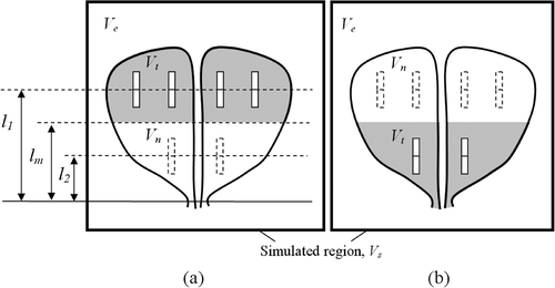
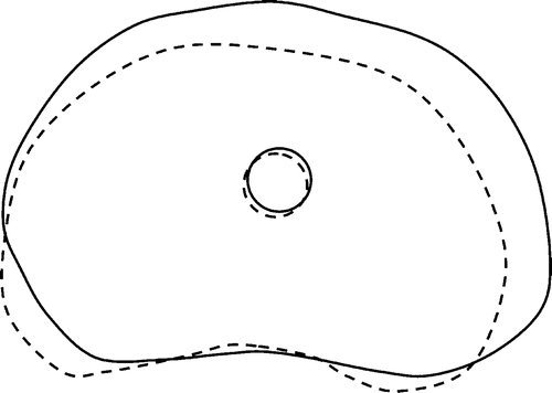
With reference to Figure 1, the prostate model is divided into two regions, one close to its base (Region I) and the other close to its apex (Region II), separated by a plane perpendicular to the direction of cryoprobe insertion at a depth l_m from the apex of the prostate, which is the average of l₁ and l₂. In Stage I, the prostate region at a distance greater than l_m is defined as a target region, V_t, and the remaining portion of the prostate is defined as a neutral region for defect calculations, V_n. Conversely, in Stage II, the prostate region at a distance shorter than l_m is defined as a target region, V_t, and the remaining portion of the prostate is defined as a neutral region for defect calculations, V_n.

Figure 1. Schematic illustration of a pullback operation, where Region I is frozen first (a), followed by freezing of Region II (b).

The duration of freezing is derived from defect progression considerations, and is calculated separately for each stage. In each stage, the initial defect region equals the entire target region. As the simulated cryoprocedure of the particular stage progresses, the internal defect decreases, while an external defect begins to form at some point in time. The simulation is terminated when the sum of internal and external defects (i.e., the overall defect, G [Equation (3)]) is minimized. Due to the pullback operation, the neutral region is excluded from evaluation of the total defect.

Once evaluation of the defect region for each stage is completed, the total defect, G_total, is calculated as the union of the internal and external defects from both freezing stages:where D_int,N and D_ext,N are the internal and external defects at the end of Stage N, and V is the volume of the defect.

Bubble packing of pullback operation

Bubble packing at a single insertion depth

Research on bubble packing at a single insertion depth has been published elsewhere [12], [13], and is presented here in brief to make the presentation complete. The bubble-packing scheme first generates ellipsoidal elements (or bubbles) inside the domain, each representing one cryoprobe at its center. Here, the ellipsoidal shape is taken as a first-order approximation of the early stage of freezing around an isolated cryoprobe. Next, van der Waals-like forces are assumed to move these bubbles to a force-balancing configuration. The van der Waals-like force model represents proximity-based attraction and repulsion forces between each pair of adjacent bubbles in the domain, where attraction forces are exerted at a long distance, and repulsion forces at a short distance. It is the combined forces among all the bubbles in the domain that eventually lead to the equilibrium layout.

In the current study, the van der Waals model is simplified tohaving the following boundary conditions:where l is the distance between two interacting bubbles, l₀ is the equilibrium distance if only two isolated bubbles are interacting, κ₀ is the a linear spring constant at distance l₀, and α, β, γ and ε are the coefficients of the simplified van der Waals attraction-repulsion force function.

The motion of bubbles towards a force-balancing configuration is simulated as a relaxation process of a second-order system:where x_i is the location of the i-th bubble, and m_i and c_i are the mass and damping coefficients of the i-th bubble, respectively. Note that m_i and c_i are assumed from computational convergence considerations, but their actual value has no physical meaning in the context of cryosurgery. Further note that f_i(t) is the sum of all inter-bubble forces acting on the i-th bubble. Equation (5) is numerically integrated using the fourth-order Runge-Kutta method [19].

Finally, the volume of the bubbles is adjusted to minimize both gaps and overlaps between bubbles as the relaxation process progresses. One possible criterion for the optimal bubble size is the amount of overlap between a bubble and its neighbors [8]:where α_i measures the overlap ratio for the i-th bubble, the index j represents a neighboring bubble, d is the diameter of the ellipsoid along the axis directed from the center of the bubble to the center of the neighboring bubble, x is the location, and n is the number of neighbor bubbles. The overlap ratio for an ideal, tightly packed configuration of bubbles in a 3D problem is 12. In the current study, the size of the bubbles is adaptively adjusted to bring the overlap ratio as close as possible to that ideal value. Once the system reaches equilibrium of inter-bubble forces for a given size of bubbles, the overlap ratio is calculated, and the diameter of the bubbles in all axes is modified according to

The change in the diameter causes changes in the inter-bubble forces, which leads to a consecutive force-relaxation process. The sequence of bubble-size modification and force relaxation continues until the bubble size converges.

Consistent with the approximation method of the frozen region to an ellipsoid, as described in reference [13], an axis ratio of 1:0.79 was taken for the ellipsoidal bubble, representing the location of the −22°C isotherm (i.e., the target isotherm for planning) at the end of 500 seconds of bioheat transfer simulation around a single cryoprobe.

Coupling bubble packing from the two stages

Due to clinical constraints, the cryoprobes in Stage II share the same placement coordinates with some cryoprobes from Stage I on the plane perpendicular to their insertion direction; fewer cryoprobes are activated in Stage II, which is smaller than Region I. The unique contribution of the current study is the technique for efficiently packing bubbles in both stages simultaneously, given the change in the number of cryoprobes between stages. For this purpose, bubbles are packed in the reverse order to that used in the pullback clinical application: bubble packing is first executed at a pre-defined insertion depth, l₂, as shown in Figure 2a, and consecutively at a pre-defined insertion depth, l₁, as shown in Figure 2b. Next, each Stage II bubble is paired with the closest Stage I bubble, thereby creating bubble couples, as shown in Figure 2c. The reverse packing order ensures that the bubble couples always lie within the boundary of Region II.

Figure 2. Schematic illustration of the process to determine the initial positions of bubbles in Stage II of pullback, where the upper illustrations display the cross-section perpendicular to the cryoprobe axis, and the lower illustrations display longitudinal cross-sections of the prostate: (a) independent Stage II bubble packing; (b) independent Stage I bubble packing; and (c) based on proximity on the plane perpendicular to the direction of cryoprobe insertion bubbles are paired, and simultaneous bubble packing is performed in both regions.

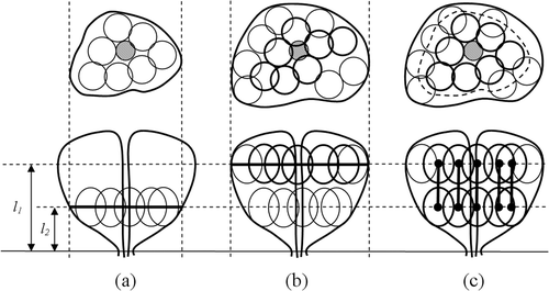
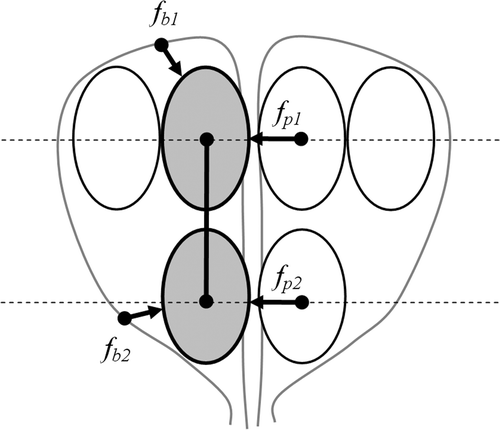
Finally, bubble packing is executed one more time on all the bubble couples and the remaining single bubbles of Stage I, as illustrated in Figure 3. Here, the overall force applied to a bubble couple is the sum of all forces from other bubbles, as well as boundary points, based on the proximity to the bubbles of Stages I and II:where f_p,N, and f_b,N represent the forces from the neighbor bubbles and the force from the boundary of Region N, calculated with Equations (5) and (6). Note that during the last stage of simultaneous bubble packing, the distance from a Stage I bubble to a Stage II bubble in the direction of cryoprobe insertion does not affect the potential force defined in Equations (5) and (6), nor does it affect the bubble-sizing function defined in Equations (8) and (9). Hence, a Stage I bubble and a Stage II bubble may freely overlap, which is consistent with clinical practice — some internal regions may experience two freezing cycles as a result of the two freezing stages.

Figure 3. Schematic illustration of forces acting on a pair of bubbles.

Results and discussion

Computerized planning in this study is demonstrated on four prostate models reconstructed from ultrasound images. Available ultrasound data included a gray-scale array of pixels for each model, having an average size of 804 (longitudinal) ×410(y) × 336(z). Approximately ten transverse cross sections were generated from each array, and 10 to 15 points were marked manually along the contour of each transverse cross section. Using the manually picked contours, the prostate shape was then reconstructed by fitting piecewise third-order Bezier surfaces [13]. Generation of a prostate model took approximately ten minutes. Since a urethral warmer was not present during imaging of any of the prostates, modeling of the urethral warmer was added as a tube 6 mm in diameter, in which the centerline coincides with the center of the urethra, as identified from imaging. The resulting volume and length of each prostate is listed in Table II for reference; the average volume was 55.9 cm³ and the average length was 48.6 mm. Figure 4 displays a 3D rendering of one of the prostates, including the urethral warmer and a cryoprobe layout, via bubble packing, using 14 cryoprobes in Stage I and 7 cryoprobes in Stage II.

Figure 4. Reconstructed prostate (model B), combined with an assumed urethral warmer and a cryoprobe layout based on bubble-packing results for 14 cryoprobes in Stage I and 7 cryoprobes in Stage II. [Color version available online.]

Consistent with previous numerical work [17], the simulated domain was selected to have a transverse cross-sectional area 3.5 times larger than the largest cross-sectional area of the specific prostate model, and the length of the domain was selected to be 1.5 times that of the same prostate model. These dimensions satisfy an underlying assumption that the human body behaves as an infinite domain in the thermal sense, when compared with the prostate in terms of size. The domain was discretized with variable grid intervals for the purpose of numerical simulations, as discussed in reference [17]. Applying typical parameters for a Joule-Thomson-based cryoprobe for cryosurgical simulation, the temperature of each cryoprobe was assumed to decrease linearly with temperature, starting with an initial temperature of 37°C, and reaching −145°C in 30 seconds; the cryoprobe temperature was assumed to be constant thereafter. Case studies included 8 to 14 cryoprobes in Stage I, and half that number of cryoprobes were assumed to be pulled back in Stage II (see Table II). In addition, a case study on the number of pulled-back cryoprobes was performed, for a maximum number of 14 cryoprobes and a variable number in Stage II of 4, 7, 11 or 14 (see Table III). All cryoprobes of the same stage are assumed to operate simultaneously. A diameter of 1.5 mm and an active length of 15 mm were assumed for each cryoprobe. The temperature in the entire simulated domain was assumed to be uniform, at the normal core body temperature of 37°C, at the beginning of either stage. Note that in clinical practice, the initial temperature in Stage II may be lower than the normal core body temperature, but above freezing (0°C), since only the freezing front location - and not temperatures - can be identified with the ultrasound imaging device used for cryosurgery. This effect is assumed to be negligible for planning purposes, as most of the heat transfer during cryosurgery goes to phase change [16].

Table II.  Summary of prostate model dimensions and pullback planning results. V_P is the prostate volume, L_P is the prostate length, L_V2 is the distance from the apex of the prostate to a plane dividing the prostate into two sections of identical volume, P₁ is the number of cryoprobes in Stage I, P₂ is the number of active cryoprobes in Stage II, l₁ is the optimal insertion depths for Stage I, l₂ is the optimal insertion depths for Stage II, G_total is the overall defect taking into account both stages, ΔG is the difference between G_total and a corresponding defect of a non-pullback case, t_BP is bubble-packing runtime, and t_HT is the combined runtime of the bioheat transfer simulation from both stages.

Prostate model	Prostate dimensions	P1	P2	l1 [mm] (l1/LP)	l2 [mm] (l2/LP)	Gtotal [%]	ΔG [%]	tBP [s]	tHT [s]
	VP = 44.4 ml^2	8	4	29 (0.65)	16 (0.35)	29.2	−0.3	19	349
A	LP = 44.5 mm	10	5	29 (0.65)	16 (0.35)	27.3	3.5	18	249
	LV = 26 mm	12	6	29 (0.65)	13 (0.30)	25.5	−1.1	23	182
		14	7	33 (0.75)	18 (0.40)	24.4	−2.1	27	220
	VP = 62.8 ml^2	8	4	32 (0.65)	15 (0.30)	30.6	2.2	17	877
B	LP = 49.9 mm	10	5	32 (0.65)	17 (0.35)	27.9	3.2	12	703
	LV2 = 28 mm	12	6	32 (0.65)	12 (0.25)	25.7	−0.3	25	324
		14	7	32 (0.65)	15 (0.30)	25.1	−1.4	20	328
	VP = 73.6 ml^2	8	4	29 (0.55)	16 (0.30)	31.9	5.7	17	1501
C	LP = 52.9 mm	10	5	29 (0.55)	16 (0.30)	22.9	−4.3	24	1153
	LV2 = 27 mm	12	6	32 (0.60)	19 (0.35)	25.6	−0.8	21	960
		14	7	29 (0.55)	13 (0.25)	24.5	−3.9	31	457
	VP = 42.8 ml^2	8	4	33 (0.70)	16 (0.35)	31.5	4.2	17	303
D	LP = 47.0 mm	10	5	31 (0.65)	14 (0.30)	27.5	0.3	21	212
	LV2 = 28 mm	12	6	33 (0.70)	16 (0.35)	25.4	−3.4	21	203
		14	7	31 (0.65)	14 (0.30)	24.7	−6.3	21	193

Table III.  Summary of results for 14 cryoprobes in Stage I and a variable number of cryoprobes in Stage II. P₂ is the number of active cryoprobes in Stage II, l₁ is the optimal insertion depths for Stage I, l₂ is the optimal insertion depths for Stage II, and A₁ and A₂ are the cross-sectional areas at depths of l₁ and l₂, respectively.

Prostate model	P2	Gtotal [%]	l1 [mm] (l1/LP)	l2 [mm] (l2/LP)	A1 [cm^2]	A2 [cm^2]	A2/A1
A	4	27.7	29 (0.65)	13 (0.30)	13.8	9.4	0.68
7	24.4	33 (0.75)	18 (0.40)	13.5	11.7	0.87
11	24.4	31 (0.70)	16 (0.35)	13.7	10.5	0.77
14	31.0	29 (0.65)	16 (0.35)	13.8	10.5	0.76
B	4	28.2	30 (0.60)	12 (0.25)	17.4	10.0	0.57
7	25.1	32 (0.65)	15 (0.30)	17.5	11.7	0.67
11	24.1	32 (0.65)	15 (0.30)	17.5	11.7	0.67
14	25.3	32 (0.65)	17 (0.35)	17.5	14.2	0.81
C	4	27.1	29 (0.55)	13 (0.25)	22.1	12.1	0.54
7	24.5	29 (0.55)	13 (0.25)	22.1	12.1	0.54
11	24.0	32 (0.60)	19 (0.35)	21.4	17.9	0.84
14	25.0	32 (0.60)	19 (0.35)	21.4	17.9	0.84
D	4	27.9	33 (0.70)	16 (0.35)	13.1	8.9	0.68
7	24.7	31 (0.65)	14 (0.30)	13.0	7.3	0.56
11	25.4	33 (0.70)	16 (0.35)	13.1	8.9	0.68
14	27.0	33 (0.70)	16 (0.35)	13.1	8.9	0.68

Cryosurgery planning with the pullback operation was compared with planning of a non-pullback operation [12]. Cryoprobes with the same diameter of 1.5 mm but an active length of 25 mm were used for the non-pullback cases, and the number of cryoprobes used in the non-pullback operation was equal to the number used in Stage I of the respective pullback case. Longer cryoprobes were selected in the non-pullback operation to compensate for the absence of an additional degree of freedom in the two-stage operation. While the active length can play a significant role in cryosurgical planning, in both pullback and non-pullback operations, further study of the active-length effect was deemed unnecessary for this proof-of-concept report.

All runtime results presented in this study were based on an AMD Athlon (TM) XP 3000+ computer, having a 2.1-GHz processor, a 400-MHz front side bus, and 1 GB of PC3200 DDR memory. The computerized planning system was implemented with Visual C++.NET and was executed using Windows XP Professional.

Insertion depth effect

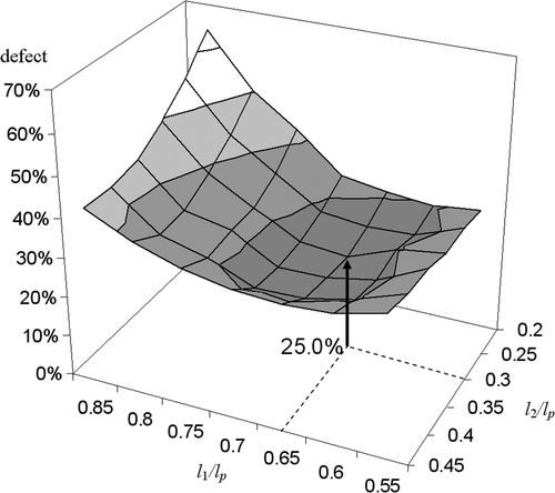
The insertion depth effect was studied using a sequence of bubble-packing planning procedures, while varying the insertion depth in each stage by intervals equivalent to 5% of the entire prostate length. At the end of each bubble-packing procedure, a bioheat transfer simulation was executed, and the total defect region was evaluated. Seeking insertion depth values that minimize the total defect is a 2D optimization problem with l₁ and l₂ as design variables. Typical results for the dependency of the total defect upon the insertion depths in Stages I and II are displayed in Figure 5. These are results for prostate model B when using 14 cryoprobes in Stage I and seven cryoprobes in Stage II. The results suggest that the global minimum can easily be found; for this specific case, the minimum was found at l₁/L_p = 0.67 and l₂/L_p = 0.3, respectively. Optimum insertion distances for other prostate models and different numbers of cryoprobes are found within a close range, as can be seen from the values listed in Tables II and III.

Figure 5. A 2D surface illustrating the total defect as a function of insertion depths in both stages for prostate model B using 14 cryoprobes in Stage I and 7 cryoprobes in Stage II.

Since bubble packing is a volumetric operation, it may be assumed that the optimal insertion depths are associated with volumetric considerations. For the purpose of studying this assumption, the distance from the apex of the prostate to a plane splitting the volume of the prostate into two segments with identical volumes, L_V2, is also listed in Table II for all cases. As expected, it can be seen from Table II that the optimal l₁ value is always greater than L_V2, and the optimal l₂ value is always smaller than L_V2; however, the difference between l₂ and L_V2 is far more significant than the difference between L_V2 and l₁, suggesting that the insertion depth is also significantly dependent on the shape and not just on the volume of the prostate.

It can further be seen from Table II that the optimal insertion depth to prostate length ratios, l₁/L_P and l₂/L_P, are 0.64 ± 0.06 and 0.32 ± 0.04, respectively; these ratio are not significantly affected by the number of cryoprobes. This observation - that the optimum insertion depth is not a strong function of the number of cryoprobes - is consistent with a previous report on non-pullback planning [12]. It is interesting that an optimum insertion depth ratio of 0.6 was found for the non-pullback operation [12], which is not significantly different from the insertion depth ratio in Stage I of the pullback operation reported in the current study, despite the difference in cryoprobe length.

Number of cryoprobes effect

In order to study the effect of the relative number of cryoprobes used in Stages I and II (P₁ and P₂, respectively), computerized planning was performed for each prostate model, with P₁ equal to 14 and a variable P₂ value of 4, 7, 11 and 14, as listed in Table III. The minimum defect values were found for cases with P₂ = 7 or 11, with marginal differences between the two general cases. It can be seen from Table III that pulling back only four cryoprobes, or all the cryoprobes, produces a noticeably greater defect. Also listed in Table III are the cross-sectional areas of each prostate, A₁ and A₂, at insertion depths l₁ and l₂, respectively; these areas are calculated at the insertion depth associated with the minimum defect achieved with respect to P₂. The A₂ to A₁ ratio suggests that P₂ should be between 0.56P₁ and 0.87P₁, if one assumes a correlation between the cross-sectional area of the prostate at a specific depth of insertion and the number of cryoprobes applied at the same depth. It is noted that the orientation of the prostate with respect to the cryoprobe insertion direction, the local curvature of the prostate surface, and geometry of the urethra also play key roles in planning, with an example of the change in the cross-sectional area at different insertion depths being displayed in Figure 6. The effect of each of these factors on planning is beyond the scope of the current proof-of-concept study. In the present study, it is suggested that a P₂ to P₁ ratio in the range of 0.5 to 0.8 (7/14 to 11/14, respectively) may yield optimum planning results, based on analysis of bioheat transfer simulations.

Figure 6. Contours of the prostate cross-section and the urethral warmer location for prostate model B, using 14 cryoprobes in Stage I and 7 cryoprobes in Stage II: l₁ = 32 mm (solid line) and l₂ = 15 mm (dashed line).

Comparison of pullback operation with non-pullback operation

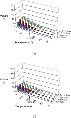
Figures 7 and 8 display representative temperature volume histograms (TVH) in the target region and external region, respectively, both for prostate model B. In the non-pullback cases, more than 75% of the target volume is simulated as having temperatures below the isotherm for planning, −22°C, and an external defect volume of less than 10%. In the pullback cases, however, a higher percentage of the target region is simulated as being below −22°C, and the external defect is found to be slightly larger; these differences are more noticeable when a greater number of cryoprobes is used. This indicates that a greater portion of the target region is cooled to lower temperatures in the pullback operation, while compromising on potentially greater cryoinjury damage to the surrounding healthy tissue.

Figure 7. Temperature volume histogram of the target region for pullback cases with 15-mm cryoprobes (a), and non-pullback cases with 25-mm cryoprobes (b), where the defect volume is normalized with respect to the prostate volume (prostate model B, Table II).

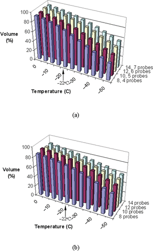
Figure 8. Temperature volume histogram of the external region for pullback cases with 15-mm cryoprobes (a), and non-pullback cases with 25 mm cryoprobes (b), where the defect volume is normalized with respect to the prostate volume (prostate model B, Table 2).

Consistent with our previous reports [12], [13], the runtime of bubble packing for the pullback operation was always significantly shorter than the execution of the bioheat transfer simulation.

Figure 9 displays the temperature field plotted on the contour of the target region for prostate model B, using 14 cryoprobes in Stage I and seven cryoprobes in Stage II. It can be seen from Figure 9 that areas having temperatures as low as the lethal temperatures are found on the contour of the target region, indicating a significant risk for cryoinjury to the surrounding healthy tissue in both pullback and non-pullback cases. The effect of Stage II is clearly observed around the apex, where the apex region possesses temperatures between −22°C and 0°C in the pullback case, while the same area possesses temperatures above 0°C in the non-pullback case. It follows that, while the defect region is a useful target function for planning, either the cryosurgeon's experience must be combined in an interactive manner, or more rules must be incorporated in the planning. For example, the defect distribution can be included as another planning parameter, favoring uniform defect distribution along the prostate contour, rather than large defects in smaller areas, as can be observed in Figure 9. Introducing more rules into the target function will be the subject of future studies, now that a proof of concept for computerized planning of cryosurgery with pullback has been demonstrated.

Figure 9. Temperature field illustrated on the surface of the reconstructed prostate, where blue represents areas with temperatures below −45°C, green represents 0°C, and red represents 37°C: (a) front view of pullback case; (b) front view of non-pullback case; (c) back view of pullback case; and (d) back view of non-pullback case, all for prostate model B. [Color version available online.]

Summary and conclusions

As part of ongoing efforts to develop clinically relevant tools for computerized planning of cryosurgery, the current study focuses on the planning of a pullback operation. Cryoprobe layout for a pullback operation was achieved by a modification of the bubble-packing method, which has been previously reported as an efficient method for planning in non-pullback cases.

Bubble packing was studied on four prostate models, reconstructed from ultrasound images. The quality of planning was evaluated based on bioheat transfer simulations. On average, a combination of the optimum cryoprobe insertion depths was found at approximately 0.64 × the prostate length - as measured from the apex of the prostate - for Stage I, and 0.32 × the prostate length for Stage II. An optimum insertion depth ratio of 0.6 was found for the non-pullback operation. The ratio of the number of cryoprobes in Stage I to those in Stage II is found to be in the range of 0.5 to 0.8.

Compared to the non-pullback operation using the same number of 25-mm cryoprobes, the cryosurgical simulation using the pullback operation achieved cooling of a greater target volume (around 80% of the prostate) below the isotherm for planning, −22°C, while damaging slightly more surrounding healthy tissues. The isotherm for planning can be adjusted by the surgeon to control the extent of the safety margins, either exterior or interior to the target region. Nevertheless, it is evident that the pullback procedure is superior to the non-pullback procedure, with defect of only a few percent, and only when a large number of cryoprobes are used in Stage II. This suggests that using a prostate-specific cryoprobe length may improve the outcome of the procedure while reducing its duration.

Acknowledgments

This project is supported by the National Institute of Biomedical Imaging and Bioengineering (NIBIB)–NIH, grant # R01-EB003563-01,02,03. We would like to thank Dr. Aaron Fenster of the Robarts Imaging Institute, London, Ontario, Canada, for providing ultrasound images. We would also like to thank Dr. Ralph Miller of Allegheny General Hospital, Pittsburgh, Pennsylvania, for clinical advice.

References

- Gage AA, Baust J. Mechanisms of tissue injury in cryosurgery. Cryobiology 1998; 37: 171–186
- Onik GM, Cohen JK, Reyes GD, Rubinsky B, Chang ZH, Baust J. Transrectal ultrasound-guided percutaneous radical cryosurgical ablation of the prostate. Cancer 1993; 72(4)1291–1299
- Cohen TK, Miller RJ, Shumarz BA. Urethral warming catheter for use during cryoablation of the prostate. Urology 1995; 45: 861–864
- Keanini RG, Rubinsky B. Optimization of multiprobe cryosurgery. ASME Transactions. J Heat Transfer 1992; 114: 796–802
- Baissalov R, Sandison GA, Donnelly BJ, Saliken JC, McKinnon JG, Muldrew K, Rewcastle JC. A semi-empirical treatment planning model for optimization of multiprobe cryosurgery. Phys Med Biol 2000; 45: 1085–1098
- Baissalov R, Sandison GA, Reynolds D, Muldrew K. Simultaneous optimization of cryoprobe placement and thermal protocol for cryosurgery. Phys Med Biol 2001; 46: 1799–1814
- Lung DC, Stahovich TF, Rabin Y. Computerized planning for multiprobe cryosurgery using a force-field analogy. Comput Methods Biomech Biomed Eng 2004; 7(2)101–110
- Shimada K. Physically-based mesh generation: Automated triangulation of surfaces and volumes via bubble-packing. Massachusetts Institute of Technology, Cambridge, MA 1993, Ph.D. thesis
- Shimada K, Gossard D. Automatic triangular mesh generation of trimmed parametric surfaces for finite element analysis. Computer Aided Geometric Design 1998; 15(3)199–222
- Yamakawa S, Shimada K (2000) High quality anisotropic tetrahedral mesh generation via packing ellipsoidal bubbles. Proceedings of the 9th International Meshing Roundtable, New Orleans, LA, October, 2000. Sandia National Laboratories, Albuquerque, NM, 263–273
- Tanaka D, Shimada K, Rabin Y. Two-phase computerized planning of cryosurgery using bubble-packing and force-field analogy. J Biomech Eng 2006; 128(1)49–58
- Tanaka D, Shimada K, Rossi M, Rabin Y. Cryosurgery planning using bubble packing in 3D. Comput Methods Biomech Biomed Eng 2007, (In press)
- Tanaka D, Shimada K, Rossi MR, Rabin Y. Towards intra-operative computerized planning of cryosurgery. Int J Med Robotics Comput Assisted Surg 2007; 3: 10–19
- Zisman A, Pantuck AJ, Cohen JK, Belldegrum AS. Prostate cryoablation using direct transperineal placement of ultrathin probes through a 17-gauge brachytherapy template - technique and preliminary results. Urology 2001; 58: 988–993
- Pennes HH. Analysis of tissue and arterial blood temperatures in the resting human forearm. J App Phys 1948; 1: 93–122
- Rabin Y, Shitzer A. Numerical solution of the multidimensional freezing problem during cryosurgery. ASME Transactions. J Heat Transfer 1998; 120: 32–37
- Rossi MR, Tanaka D, Shimada K, Rabin Y. An efficient numerical technique for bioheat simulations and its application to computerized cryosurgery planning. Computer Methods and Programs in Biomedicine 2007; 85(1)41–50
- Turk TMT, Rees MA, Myers CE, Mills SE, Gillenwater JY. Determination of optimal freezing parameters of human prostate cancer in a nude mouse model. Prostate 1999; 38: 137–143
- Press WH. Numerical Recipes in C: The Art of Scientific Computing. Cambridge University Press, Cambridge, MA 1988
- Rabin Y, Stahovich TF. The thermal effect of urethral warming during cryosurgery. CryoLetters 2002; 23: 361–374
- Rabin Y. A general model for the propagation of uncertainty in measurements into heat transfer simulations and its application to cryobiology. Cryobiology 2003; 46(2)109–120
- Altman PL, Dittmer DS. Respiration and Circulation (Data Handbook). Federation of American Societies for Experimental Biology, Bethesda, MD 1971