Mean-shifted surface curvature algorithm for automatic bone shape segmentation in orthopedic surgery planning: a sensitivity analysis

Abstract

The results of recent studies concerning statistical bone atlases and automated shape analysis are promising with a view to widening the use of surface models in orthopedic clinical practice, both in pre-operative planning and in the intra-operative stages. In this domain, automatic shape analysis is strongly advocated because it offers the opportunity to detect morphological and clinical landmarks with superior repeatability in comparison to human operators. Surface curvatures have been proposed extensively for segmentation and labeling of image and surface regions based on their appearance and shape. The surface curvature is an invariant that can be exploited for reliable detection of geometric features. In this paper, we investigate the potentiality of the algorithm termed mean-shift (MS), as applied to a non-linear combination of the minimum and maximum curvatures of a surface. We exploited a sensitivity analysis of the algorithm parameters across increasing surface resolutions. Results obtained with femur and pelvic bone surface data, reconstructed from cadaveric CT scans, demonstrated that the information content derived by the MS non-linear curvature overcomes both the mean and the Gaussian curvatures and the original non-linear curvature. By applying a threshold-based clustering algorithm to the curvature distribution, we found that the number of clusters yielded by the MS non-linear curvature is significantly lower (by a factor of up to 6) than that obtained by using the original non-linear curvature. In conclusion, this study provides valuable insights into the use of surface curvature for automatic shape analysis.

• Surface curvature
• mean-shift
• vertex clustering
• acetabulum
• hip joint replacement
• orthopedic surgical planning

Introduction

The results of recent studies concerning statistical bone atlases and automated shape analysis are promising with a view to widening the use of surface models in orthopedic clinical practice, both in pre-operative planning and in the intra-operative stages [1–5]. Statistical models of bone structures have been investigated extensively with the aim of enhancing automation in CT and MR image segmentation [6–12] and reconstructing patient-specific shape models from a small number of X-ray images or even from a single image [13–15]. Innovative methods for bone shape analysis have been applied to 3D mesh segmentation and clinical feature detection [16–21]. In this domain, automatic shape analysis is strongly advocated because it offers the opportunity to detect morphological and clinical landmarks (MCL) with superior repeatability in comparison to human operators. It has been shown that manual interaction is commonly time consuming, and that the results are mostly dependent upon the examiner's individual expertise and are affected by noticeable inter-observer variability [22–25].

Invariant geometric measures such as curvatures, extreme points, and higher-order derivatives have been proposed for segmenting and labeling bone surface regions based on their appearance and shape [16], [26–29]. Specifically, the surface curvature is an invariant, independent of position and orientation, that can be exploited for reliable detection of geometric features as concavities and convexities. The advantage of this is that the magnitude provides a direct measurement of the saliency of both points and regions that are anatomically and clinically relevant. In fact, while smooth portions of the bony shapes lead to near-zero curvature values, uniformly curved and abrupt local variation areas are clearly characterized by curvature extremes, which can be alternatively classified as pit/valley and ridge/peak regions [30]. In addition, curvature is a local measure, in the sense that a small perturbation or a morphological variation confined to a narrow region has limited spatial effect over the shape description. For such reasons, surface curvature has been widely proposed as a shape descriptor and investigated for the automatic extraction of MCL. It has been applied to the analysis of patterns of cranial morphological differentiation in rodent species [30] and for MCL detection in femur and pelvic bone models [29], [31]. However, in using surface curvature to detect MCL in bone shapes, two main issues have to be addressed. Firstly, point landmarks result in wider areas rather than easily identifiable discrete points. In addition, because there are no clear geometric separations between morphological regions, region clustering can lead to either over- or under-estimation. Secondly, morphological variability and shape degeneracy in the presence of pathologic conditions, along with 3D reconstruction noise and surface resolution, reduce the reliability of the curvature assessment and the region clustering. As a result, classical shape curvature descriptors can be insufficient for automatic clustering, and knowledge-based clustering techniques, with manual threshold set-up, are better suited in this regard.

In this work, we address the issue of robust surface curvature assessment by investigating the potentiality of the mean-shifted curvature algorithm, proposed by Zhang et al. [32], as applied to pelvic and femur bone shapes for virtual surgery planning. The mean-shift curvature algorithm is a non-parametric mode finding/clustering procedure for iteratively refining the curvature values of a mesh. It takes its root from the general mean-shift approach to multimodal function smoothing. Technically, a general mean-shift algorithm treats the points in an n-dimensional feature space Ω as an empirical probability density function, where dense regions in the feature space correspond to the local maxima or modes of the underlying distribution [33–35]. Given a sample point of the feature space, the mean-shift algorithm first estimates the density of the feature space, then evaluates the gradient of the density function, and then performs a gradient ascent on the local estimated density until convergence. The stationary points of this procedure represent the modes of the distribution. Furthermore, the data points associated (at least approximately) with the same stationary point are considered to be members of the same cluster. A standard mean-shift algorithm is generally guaranteed to be convergent [34]. This technique has been successfully used in image segmentation, image blurring correction, and video object tracking. It has also been applied to feature space analysis of 3D meshes, and to feature extraction, data exploration, and model partitioning, exploiting a geodesic parameterization of the mesh to obtain a uniform feature space for spatial information and the other mesh feature [36–38]. In reference 32, Zhang et al. showed that superior surface clustering performance can be attained by using the mean-shifted curvature. However, the generality of the approach was not demonstrated. In our study, we performed a sensitivity analysis of the main algorithm parameters as a function of the surface detail (i.e., the number of mesh faces) and analyzed how automatic region clustering is facilitated.

Material and methods

Curvature estimation on surface mesh

The curvature at any point on a surface corresponds to how the tangent vector changes as one moves infinitesimally along a chosen curve on the surface. Thus, each point has, in principle, an infinite number of curvatures, each corresponding to a specific direction. The maximum and minimum curvatures (which may be equal) are called the principal curvatures. Using these principal curvatures, we can derive various indices that provide some information about the local shape of the surface. In the specific case of a surface mesh composed of triangles, the principal curvatures of the surface mesh can be easily computed [39]. Let and be a set of all triangular faces adjacent to vertex , with V being the set of the r mesh vertices, and the normal direction to the face , respectively. The vertex normal is defined as the weighted average of the normal directions of its adjacent faces. Considering as the centroid of face , the vertex normal can be computed as follows:

For , the set of vertices adjacent to (1-ring), a unit tangent associated to is defined as the normalization of the projection of on the tangent plane of . The normal curvature of along can be then approximated by

Without loss of generality, let be the maximum among all these values. Denoting as the angle between and , can be then expressed aswhere and b and c can be estimated by least-square fitting. The Gaussian , the mean , and the two principle curvatures and at the vertex can be computed as follows:

To amplify the difference between convex and concave regions, the curvature, obtained as a nonlinear function of the minimum and maximum curvatures, can be used [30], [40]:

Positive values of , lower than 1, identify ridge and peak regions; conversely, negative values, greater than −1, identify pit and valley regions. A further curvature enhancement is yielded by applying the mean-shift (MS) approach as used in the field of data clustering using multivariate kernel density estimates. In the basic representation, considering r data points , the multivariate kernel density estimate using a kernel, , is given bywhere a_i, termed the bandwidth parameter and dependent on the i-th point, defines the range of the kernel. Among different potential solutions, a constant bandwidth parameter a is usually chosen heuristically [35]. Traditionally, radial symmetric kernels are adopted aswith p being a normalization factor assuring that F(x) integrates to 1. The most-used kernels are the uniform, the Epanechnikov, the biweight, the Gaussian, and the triangular. In particular, the following general functionwhere , which holds for , can be specialized in the uniform (c = 0), the Epanechnikov (c = 1), and the biweight (c = 2) kernels.

The mean-shift (MS) algorithm requires determination of the gradient of the density function estimator (Equation 6). The mean-shift vector points toward the direction of the maximum increase in density, and is proportional to the density gradient estimate at point obtained with the kernel .

In our specific case, the feature space is a joint domain involving two components, namely the 2D manifold (spatial coordinates of the vertices), embedded in 3D space, and the 1D curvature.

A generalized bivariate mean-shift density function [35] can be then defined aswhere and are the two kernel functions, a and b are the constant bandwidth parameters, and r is the number of mesh vertices. To simplify the density function without losing generality, the kernel can be set to a flat function and the bandwidth parameter can be set to a constant, i.e., for and 0 otherwise. For mesh surfaces, the integer value of t corresponds to updating the curvature of a vertex with that of its t-ring vertices. The degree of curvature smoothness yielded is just the right function of the vertex neighborhood. By setting a = 2, Equation 9 simplifies further as

Assuming that is a radial symmetric kernel (Equation 8), the gradient of the curvature density of Equation 10 assumes the following shape:where andis the mean-shifted curvature at the vertex v, which does not rely on the number of vertices r in the mesh. The curvature is iteratively refined asuntil is less than a user-specified threshold , which corresponds to a lower bound for the magnitude of the mean-shift vector. The parameter was set up to 10⁻⁵. The regions of low-density values are of no interest for the feature space analysis and, in such regions, the mean-shift steps are large. Similarly, near local maxima the steps are small and the analysis more refined. The mean-shifted curvature algorithm is thus an adaptive gradient ascent method that further intensifies the difference between convex and concave regions.

Region clustering

Target regions are localized by grouping vertices and triangles based on their curvature values. Two groups of vertices are obtained according to a positive threshold and a negative threshold . In our approach, we decided to define grouping thresholds automatically computed from the positive and negative value histograms using the 75th and 25th percentile values, respectively. The vertex classification is then mapped to corresponding faces. A triangle is added to a face list if all of its three vertices are in the same group. Two face lists, namely and , are then obtained. Clustered regions consist of edge-connected faces within a list. A recursive algorithm associates edge-connected adjacent triangles and continues until no edge-connected triangle within the region remains. The process yields two groups of face clusters: one for pit regions and one for ridge regions.

Sensitivity analysis

The sensitivity analysis of the curvature estimation was evaluated by comparing the number of clusters obtained from the region clustering process after computing alternatively the curvature k_c, the 1-ring neighborhood mean-shifted k_c, and the 2-ring neighborhood mean-shifted k_c. A non-parametric statistical test (the Kruskall-Wallis test) was used with a confidence interval of 1%. Two main radial symmetric kernels (Equation 8), proposed successfully in image segmentation and analysis [35], [38], [41], were considered in this study: the Epanechnikov () and the biweight () functions. The effect of the parameter b (Equation 10) was studied in a large value range from 10² to 10⁻⁸. The analysis was performed on three different surface detail levels, corresponding to different numbers of surface faces (20000, 10000, and 3000). For each bone model, the three surfaces were obtained using the Amira software package (Visage Imaging GmbH, Berlin, Germany) by smoothing the original mesh reconstructed from CT segmentation.

Test data

The analysis was performed on two surface datasets for 20 femoral and 20 hemi-pelvic bone models. The outer bone surfaces were reconstructed from CT scans of 11 embalmed cadavers (9 males and 2 females) with an average age of approximately 77 years (range 61–95 years), using the Mimics application (Materialise NV, Leuven, Belgium). Approximately 650 contiguous axial slices (512 × 512 pixels) were acquired at 1-mm scan intervals from the upper pelvis to the proximal tibia. The segmentation of the pelvic bone and femur was performed, using manual editing, by radiological experts. The articular cartilages were excluded from segmentation. The mean number of triangles was 74337 (SD: 13241) and 81563 (SD: 12776) for the femur and pelvic bone, respectively. As two subjects underwent a total hip arthroplasty on their left and right hip, respectively, only 10 left and 10 right image datasets were considered (Table II).

Table I.  Parameters and ranges for the sensitivity analysis.

Curvature	kc	1-ring MS kc	2-ring MS kc
Surface resolution (No. of faces)	3000	10,000	20,000
Kernel function	Epanechnikov		Biweight
b	Range: 10^2 to 10^−8		Step: 10^−1

Table II.  Features of the validation data.

CT image size	512 × 512 pixels
Voxel size	0.74 × 0.74 × 1.0 mm
Demographic data	9 males, 2 females Mean age: 77 years (61–95)
Surfaces	Femur	Pelvic bone
Left	10	10
Right	10	10
No. of triangles (mean ± std)	74337 ± 13241	81563 ± 12776

Results

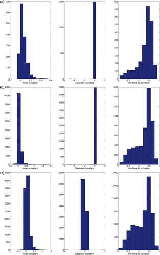
The graphical comparison between the mean (Equation 4), Gaussian (Equation 4) and non-linear k_c (Equation 5) curvatures was reported for the hemi-pelvic bone (Figure 1) and femur (Figure 2) surfaces with 3k and 20k faces. Simple visual inspection led to an appreciation that the k_c curvature better separates the convexities from the concavities than either of the other two curvature modalities. The value range of the mean and Gaussian curvatures changes with the surface detail, which is an unpleasant effect. In contrast, the k_c curvature is always in the range of (−1 … 1), no matter what the surface detail may be (see Figure 1, bottom panels). The histograms of the three curvature distributions computed for pelvic bone surface at 3k, 10k and 20k faces showed that the histogram for the non-linear k_c maintains approximately the same shape across increasing surface resolution (Figure 3). In contrast, both the mean and Gaussian curvature histograms visibly change their shapes. This in turn prevents the use of simple threshold-based clustering techniques.

Figure 1. (a) and (b) The three curvatures (from left to right: mean, Gaussian, and non-linear k_c) mapped on the pelvic bone mesh with 3k faces (a) and 20k faces (b). (c) and (d) Corresponding curvature values. For clarity, the ordinate range was set from −2 to +2.

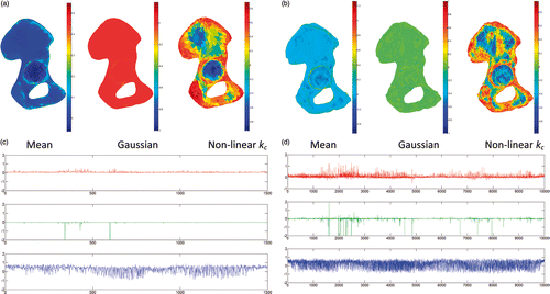
Figure 2. The three mapped curvatures (mean, Gaussian, and non-linear k_c) for the femur mesh (3k and 2k faces).

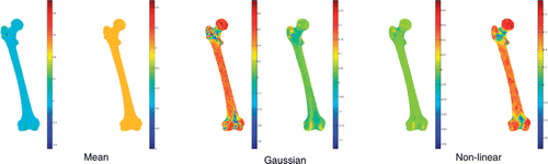
Figure 3. Histograms of the three curvature distributions (pelvic bone) computed for the 3k (a), 10k (b), and 20k (c) surface resolutions.

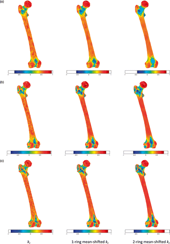
In Figures 4 and 5, the curvature k_c, 1-ring neighborhood mean-shifted k_c, and 2-ring neighborhood mean-shifted k_c are displayed for the pelvic bone and femur, respectively. As expected, both 1-ring and 2-ring MS k_c led to more uniform curvature regions than the original k_c curvature. Such an interesting outcome was more effective with increasing surface detail (cf. Figures 4c and 5c). This can be seen for the acetabular region (Figure 4c), where a clear separation between the lunate surface and the acetabular fossa was present in curvature k_c. In contrast, the smoothing effect of both 1-ring and 2-ring MS k_c was likely to reduce this difference. For the femoral surface, the effect of the MS was to improve the separation between the shaft and the distal and proximal femoral ends. Also, the curvature differences of the two condyles with respect to the frontal cortical and intercondylar fossa were enhanced.

Figure 4. Curvature k_c, mean-shifted curvature with 1-ring neighborhood, and mean-shifted curvature with 2-ring neighborhood for 3k faces (a), 10k faces (b), and 20k faces (c).

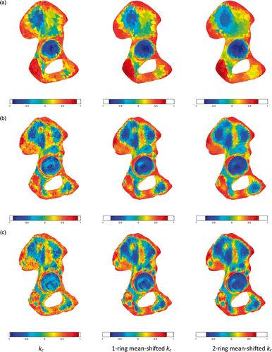
Figure 5. Curvature k_c, mean-shifted curvature with 1-ring neighborhood, and mean-shifted curvature with 2-ring neighborhood for 3k faces (a), 10k faces (b), and 20k faces (c).

The effect of the two different kernels (the Epanechnikov and biweight) in the mean-shifted curvature computation was analyzed by processing the pelvic bone surface. The results showed that the Epanechnikov kernel provides an equal number of clusters for any b value in the tested range (Table III). As expected, the number of clusters grew up along with the surface resolution for both ridge and pit regions. In contrast, for the biweight kernel, b values lower than 1 led to a dramatic increase in the number of clusters. In this case, the smoothing effect of the mean-shift algorithm on the surface curvature was visibly reduced. Using the Epanechnikov kernel with b equal to 1.00E−04, the distributions of the ridge and pit cluster number were computed for k_c, 1-ring MS k_c and 2-ring MS k_c curvatures (Tables IV and V).

Table III.  Number of clusters for ridge (R) and pit (P) regions as a function of the b value, the kernel function, and the surface resolution obtained after computing the 1-ring MS curvature, automatic curvature thresholding, and vertex clustering.

Kernel	Epanechnikov						Biweight
Surface resolution	3k		10k		20k		3k		10k		20k
b value	R	P	R	P	R	P	R	P	R	P	R	P
100	7	3	32	14	87	42	7	3	32	14	90	38
10	7	3	32	14	87	42	7	3	32	14	90	38
1	7	3	32	14	87	42	19	3	32	13	90	38
1.00E−01	7	3	32	14	87	42	23	3	122	52	107	41
1.00E−02	7	3	32	14	87	42	23	6	121	52	107	41
1.00E−03	7	3	32	14	87	42	23	6	121	52	107	41
1.00E−04	7	3	32	14	87	42	23	6	121	52	107	41
1.00E−05	7	3	32	14	87	42	23	6	121	52	107	41
1.00E−06	7	3	32	14	87	42	23	6	121	52	107	41
1.00E−07	7	3	32	14	87	42	23	4	121	52	107	41
1.00E−08	7	3	32	14	87	42	23	6	121	52	107	41

Table IV.  Median and range values (25th and 75th percentiles) for the ridge and pit cluster distributions, obtained from the pelvic bone processing, computed across the 20 bone models. For clarity, floating point numbers are rounded to the nearest integer.

		3k			10k			20k
		kc	1-ring MS kc	2-ring MS kc	kc	1-ring MS kc	2-ring MS kc	kc	1-ring MS kc	2-ring MS kc
Ridge	Median	37	15	6	74	25	13	204	82	34
	Range	34–40	13–17	10–13	71–81	19–27	10–15	199–212	79–90	22–39
Pit	Median	11	5	3	29	15	8	87	41	24
	Range	8–12	4–5	3–4	26–32	11–18	7–11	78–89	36–47	22–27

Table V.  Median and range values (25th and 75th percentiles) for the ridge and pit cluster distributions, obtained from the femur processing, computed across the 20 bone models. For clarity, floating point numbers are rounded to the nearest integer.

		3k			10k			20k
		kc	1-ring MS kc	2-ring MS kc	kc	1-ring MS kc	2-ring MS kc	kc	1-ring MS kc	2-ring MS kc
Ridge	Median	44	14	7	130	43	21	260	87	45
	Range	41–47	12–15	7–9	125–141	38–49	15–25	247–271	74–94	39–52
Pit	Median	7	5	4	20	18	14	48	41	31
	Range	5–8	4–6	3–4	19–23	16–20	13–15	44–50	37–43	25–36

As expected, a lower number of clusters was yielded for the 2-ring MS k_c in comparison to both k_c and 1-ring MS k_c for all three surface detail levels. The absolute number of clusters increased with the detail value. For the pelvic bone, the number of ridge clusters, computed using k_c, diminished by a factor of approximately 6 with respect to 2-ring MS k_c for all three resolutions, while the number of pit clusters, computed using k_c, diminished by a factor of approximately 3.5 with respect to 2-ring MS k_c for all three resolutions. For all three surface resolutions and for ridge and pit regions, the statistical difference between k_c cluster distribution and both 1-ring MS k_c and 2-ring MS k_c cluster distributions was significant. For the femur bone, the number of ridge clusters, computed using k_c, diminished by a factor of approximately 6 with respect to 2-ring MS k_c for all three resolutions. The number of pit clusters, computed using k_c, diminished by a factor of approximately 1.5 with respect to 2-ring MS k_c for all three resolutions. Again, significant statistical differences (p < 1e−3) were found for k_c, 1-ring MS k_c and 2-ring MS k_c cluster distributions.

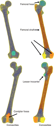
The color-coded regions clustered for the 3k-face surface of the hemi-pelvic bone (Figure 6) and femur (Figure 7), obtained after computing 2-ring MS k_c, showed clear evidence of the segmentation of relevant clinical parts in the pelvic bone (the acetabulum, pubic tubercle, posterior interior iliac spine, and anterior superior iliac spine) and in the femur (the femoral head, femoral shaft, condyles, and condylar fossa lesser trocanter).

Figure 6. Color-coded regions clustered for 3k-face surface of the hemi-pelvic bone. The upper and lower images display the anterior and posterior views, respectively.

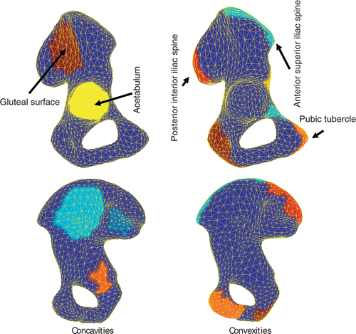
Figure 7. Color-coded regions clustered for 3k-face surface of the femur. The upper and lower images display the anterior and posterior views, respectively.

Discussion and conclusions

Virtual surgery planning is an innovative concept that is emerging in the field of orthopedics because of recent developments in automatic image processing and shape analysis. This concept includes three main steps: (1) image segmentation and surface reconstruction; (2) bone shape analysis and MCL identification; and (3) determination of prosthesis size and alignment, along with the definition of bone cuts. In this context, bone shape analysis and MCL identification play a significant role, as the quality of the third step strongly depends on them. In general, while expert guidance still seems mandatory, undue inter-operator variability is introduced into the results. Automated and even fully automatic methods are being investigated with a view to reducing operator dependence. Curvature represents one of the promising methodological approaches to the automatic identification of MCL, as it provides direct information about concavities and convexities in a surface.

In the classical approach, the mean and Gaussian curvatures were mainly used in combination to identify different region types [30], [42]. Nonetheless, as evidenced in this work, both curvatures are sensitive to surface detail level, and the region clustering cannot be straightforward (Figure 3). In reference [29], the authors used this approach to detect anatomical landmarks in the femur. However, after region clustering they introduced a knowledge-based method to remove undue clustered regions and better discriminate between concavities and convexities. The main limitation of the study was that the authors tested the approach on just a single surface model, thus the results lack generality.

In this paper, we have shown that the curvature k_c (Equation 5) can be used to increase the difference between concavities and convexities as an alternative to the mean and the Gaussian curvatures. We verified that the curvature k_c range (−1:+1) is not dependent on the surface detail, and that the histogram shape is almost identical across different surface resolutions (Figure 3). Conversely, the value ranges of the mean and Gaussian curvatures are not bounded and the histogram shapes are variable with the surface detail. As shown, however, the original curvature k_c, as it depends non-linearly on minimum and maximum curvatures, can be sensitive to surface noise. This effect is more relevant with increasing surface detail (cf. Figures 4 and 5).

We have considered a particular approach to processing the curvature k_c based on the mean-shift algorithm. As a result, we found that the curvature distribution obtained gains a considerable smoothness quality, increasing with the neighborhood used to compute the mean-shift factor (cf. Equation 10 and Figures 4 and 5). This should facilitate the following region clustering stage. Indeed, our results showed that, by applying a simple threshold-based clustering technique, the number of clusters of the MS curvature k_c was significantly lower than the number of clusters obtained using the original curvature k_c (Tables III and IV). The MS curvature algorithm was little influenced by the intrinsic parameters (kernel function and bandwidth factor b). The use of the Epanechnikov kernel led to a complete independence of the clustering results from the b factor over a large variation range (Table III). The algorithms were implemented in the MATLAB environment (MathWorks, Natick, MA). By setting the parameter to 10⁻⁵, approximately 6 iterations on average were sufficient to refine the curvature k_c at all the mesh vertices with the mean-shift algorithm. The MS curvature computation for a single 20k-face surface model took approximately 3 seconds and 17 seconds for 1-ring and 2-ring neighborhoods, respectively, on an Intel® Xeon® Quad-Core Processor W3530 (2.80 GHz, 8 MB cache, 1066 MHz memory) equipped with 4 GB RAM.

In conclusion, MS k_c represents a robust and fast computational method for estimating with high reliability the surface curvature, which can then be used for automatic region clustering in anatomical shapes. It can thus contribute greatly to advancing innovative approaches in virtual orthopedic surgery planning.

Declaration of interest: The authors report no declaration of interest.

References

- Suero EM, Hüfner T, Stübig T, Krettek C, Citak M. Use of a virtual 3D software for planning of tibial plateau fracture reconstruction. Injury 2010; 41(6)589–591
- Wong KC, Kumta SM, Leung KS, Ng KW, Ng EWK, Lee KS. Integration of CAD/CAM planning into computer assisted orthopaedic surgery. Comput Aided Surg 2010; 15(4–6)65–74
- Oka K, Murase T, Moritomo H, Goto A, Sugamoto K, Yoshikawa H. Corrective osteotomy using customized hydroxyapatite implants prepared by preoperative computer simulation. Int J Med Robotics Comput Assist Surg 2010; 6: 186–193
- Steinberg EL, Menahem A, Dekel S. Preoperative planning of total hip replacement using the TraumaCad™ system. Arch Orthop Trauma Surg 2010; 130: 1429–1432
- Fornaro J, Keel M, Harders M, Marincek B, Székely G, Frauenfelder T. An interactive surgical planning tool for acetabular fractures: Initial results. J Orthop Surg Res 2010; 5: 50
- Chintalapani G, Ellingsen LM, Sadowsky O, Prince JL, Taylor RH, Statistical atlases of bone anatomy: Construction, iterative improvement and validation. In: Ayache N, Ourselin S, Maeder AJ, editors. Proceedings of the 10th International Conference on Medical Image Computing and Computer Assisted Intervention (MICCAI 2007), Brisbane, Australia, October 29-November 2, 2007. Part I. Lecture Notes in Computer Science 4791. Berlin: Springer; 2007. pp 499–506
- Liu J, Udupa JK, Saha PK, Odhner D, Hirsch BE, Siegler S, Simon S, Winkelstein BA. Rigid model-based 3D segmentation of the bones of joints in MR and CT images for motion analysis. Med Phys 2008; 35(8)3637–3649
- Kainmüller D, Lamecker H, Zachow S, Hege H-C. An articulated statistical shape model for accurate hip joint segmentation. In: Proceedings of the 31st Annual International Conference of the IEEE Engineering in Medicine and Biology Society (EMBC2009), Minneapolis, MN, September 2009. pp 6345–6351
- Wu C, Murtha PE, Jaramaz B. Construction of statistical shape atlases for bone structures based on a two-level framework. Int J Med Robot Comput Assist Surg 2010; 6(1)1–17
- Baldwin MA, Langenderfer JE, Rullkoetter PJ, Laz PJ. Development of subject-specific and statistical shape models of the knee using an efficient segmentation and mesh-morphing approach. Comput Methods Programs Biomed 2010; 97(3)232–240
- Ramme AJ, Criswell AJ, Wolf BR, Magnotta VA, Grosland NM. EM segmentation of the distal femur and proximal tibia: A high-throughput approach to anatomic surface generation. Ann Biomed Eng 2011; 39(5)1555–1562
- Schmid J, Kim J, Magnenat-Thalmann N. Robust statistical shape models for MRI bone segmentation in presence of small field of view. Med Image Anal 2011; 15(1)155–168
- Skalli W, De Guise JA. A hierarchical statistical modeling approach for the unsupervised 3-D reconstruction of the scoliotic spine. IEEE Trans Biomed Eng 2005; 52: 2041–2057
- Zheng G. Statistically deformable 2D/3D registration for estimating post-operative cup orientation from a single standard AP X-ray radiograph. Ann Biomed Eng 2010; 38(9)2910–2927
- Zheng G, von Recum J, Nolte LP, Grützner PA, Steppacher SD, Franke J. Validation of a statistical shape model-based 2D/3D reconstruction method for determination of cup orientation after THA. Int J Comput Assist Radiol Surg 2011 Jul 27 [Epub ahead of print]
- Xi J, Hu X, Jin Y. Shape analysis and parameterized modeling of hip joint. Trans ASME 2003; 3(9)260–265
- Subburaj K, Ravi B, Agarwal M. Automated identification of anatomical landmarks on 3D bone models reconstructed from CT scan images. Comput Med Imaging Graph 2009; 33(5)359–368
- Li K, Tashman S, Fu F, Harner C, Zhang X. Automating analyses of the distal femur articular geometry based on three-dimensional surface data. Ann Biomed Eng 2010; 38(9)2928–2936
- Cerveri P, Marchente M, Bartels W, Corten K, Simon JP, Manzotti A. Automated method for computing the morphological and clinical parameters of the proximal femur using heuristic modeling techniques. Ann Biomed Eng 2010; 38(5)1752–1766
- Cerveri P, Marchente M, Bartels W, Corten K, Simon JP, Manzotti A. Towards automatic computer-aided knee surgery by innovative methods for processing the femur surface model. Int J Med Robot Comput Assist Surg 2010; 6(3)350–361
- Cerveri P, Marchente M, Manzotti A, Confalonieri N. Determination of the Whiteside line on the femur surface model by fitting high-order polynomial functions to the cross-section profiles of the intercondylar fossa. Comput Aided Surg 2011; 16(2)71–85
- Oddy M, Jones M, Pendegrass C, Pilling J, Wimhurst J. Assessment of reproducibility and accuracy in templating hybrid total hip arthroplasty using digital radiographs. J Bone Joint Surg Br 2006; 88: 581–585
- Yau WP, Leung A, Liu KG, Yan CH, Wong LL, Chiu KY. Interobserver and intra-observer errors in obtaining visually selected anatomical landmarks during registration process in non-image-based navigation-assisted total knee arthroplasty. J Arthroplasty 2007; 22(8)1150–1161
- Morton NA, Maletsky LP, Pal S, Laz PJ. Effect of variability in anatomical landmark location on knee kinematic description. J Orthopaedic Res 2007; 25(9)1221–1230
- Taddei F, Ansaloni M, Testi D, Viceconti M. Virtual palpation of skeletal landmarks with multimodal display interfaces. Med Inform Internet Med 2007; 32(3)191–198
- Rohr K. Extraction of 3D anatomical point landmarks based on invariance principles. Pattern Recognition 1999; 32(1)3–15
- Costa L da F, dos Reis SF, Arantes RAT, Alves ACR, Mutinari G. Biological shape analysis by digital curvature. Pattern Recognition 2004; 37: 515–524
- Worz S, Rohr K. Localization of anatomical point landmarks in 3D medical images by fitting 3D parametric intensity models. Med Image Anal 2006; 10: 41–58
- Koenderink JJ, Van Doorn AJ. Surface shape and curvature scales. Image and Vision Computing 1992; 10(8)557–565
- Subburaj K, Ravi B, Agarwal M. Computer-aided methods for assessing lower limb deformities in orthopaedic surgery planning. Comput Med Imaging Graph 2010; 34(4)277–288
- Zhang X, Li G, Xiong Y, He F, 3D mesh segmentation using mean-shifted curvature. In: Chen F, Jüttler B, editors. Proceedings of the 5th International Conference on Advances in Geometric Modeling and Processing (GMP ‘08), Hangzhou, China, April 2008. Lecture Notes in Computer Science 4975. Berlin: Springer-Verlag; 2008. pp 465–474
- Cheng Y. Mean shift, mode seeking, and clustering. IEEE Trans Pattern Anal Mach Intell 1995; 17(8)790–799
- Comaniciu D, Meer P. Distribution free decomposition of multivariate data. Pattern Analysis and Applications 1999; 2: 22–30
- Comaniciu D, Meer P. Mean shift: A robust approach towards feature space analysis. IEEE Trans Pattern Anal Mach Intell 2002; 24: 603–619
- Shamir A, Shapira L, Cohen-Or D. Mesh analysis using geodesic mean-shift. The Visual Computer 2006; 22(2)99–108
- Park M, Brocklehurst K, Collins RT, Liu Y. Deformed lattice detection in real-world images using mean-shift belief propagation. IEEE Trans Pattern Anal Mach Intell 2009; 31(10)1804–1816
- Ye X, Beddoe G, Slabaugh G. Automatic graph cut segmentation of lesions in CT using mean shift superpixels. Int J Biomed Imaging 2010; 2010: 983963, (Epub)
- Dong C, Wang G. Curvatures estimation on triangular mesh. Journal of Zhejiang University (SCIENCE) 2005; 6A(S1)128–136
- Faugeras O. Three-Dimensional Computer Vision: A Geometric View-Point. MIT Press, Cambridge, MA 1993
- Tao W, Jin H, Zhang Y. Color image segmentation based on mean shift and normalized cuts. IEEE Transactions on Systems, Man and Cybernetics, Part B 2007; 37(5)1382–1389
- Yamauchi H, Gumhold S, Zayer R, Seidel H-P. Mesh segmentation driven by Gaussian curvature. The Visual Computer 2005; 21(8–10)659–668