Methods for abdominal respiratory motion tracking

Abstract

Non-invasive surface registration methods have been developed to register and track breathing motions in a patient’s abdomen and thorax. We evaluated several different registration methods, including marker tracking using a stereo camera, chessboard image projection, and abdominal point clouds. Our point cloud approach was based on a time-of-flight (ToF) sensor that tracked the abdominal surface. We tested different respiratory phases using additional markers as landmarks for the extension of the non-rigid Iterative Closest Point (ICP) algorithm to improve the matching of irregular meshes. Four variants for retrieving the correspondence data were implemented and compared. Our evaluation involved 9 healthy individuals (3 females and 6 males) with point clouds captured in opposite breathing phases (i.e., inhalation and exhalation). We measured three factors: surface distance, correspondence distance, and marker error. To evaluate different methods for computing the correspondence measurements, we defined the number of correspondences for every target point and the average correspondence assignment error of the points nearest the markers.

• Non-rigid iterative closest point
• point cloud
• respiratory motion tracking
• time-of-flight

Introduction

Respiratory motion compensation is an important problem for radiotherapy and other minimally invasive interventions [1]. The goal of our study was to track and register abdominal movements to gain better knowledge about breathing motions, to detect anomalies during breathing or respiration, and to track the human body displacement during radiotherapy. The first approach tested was to attach optical black-white markers to the abdomen to facilitate the tracking of abdominal motion using a stereo camera and triangulation reconstruction. This method allowed us to track only a few points [2]. Borgert et al. [3] used two electromagnetic tracking sensors (internal and external) to evaluate the possibility of using an external sensor for respiratory motion compensation. A 78% correlation for continuous breathing and a 94% correlation for steady respiration with or without a minimal needle for patient motion were obtained. The displacements between the estimated and measured positions were reduced from 3.90 ± 2.0 and 4.14 ± 2.10 mm, respectively, to 0.99 ± 0.66 and 0.94 ± 0.46 mm, respectively, but only for one patient. Maier-Hein et al. [4] proposed a method to estimate the movement of a target point in the liver nodule, which was based on a combination of internal and external markers. The external markers were black and white, and needles were used as internal markers. The online tracked positions of the markers were used to calculate the coefficient of the deformation field based on a free-form deformation approach, which was then used to estimate the target movement. One of the inserted needles served as a target point, and the target registration error was calculated as the difference between the measured and estimated target positions. Depending on the number of internal and external markers and the type of transformation, the target registration error (TRE) was between 1 and 5 mm. In this method, increasing the number of tracking points is difficult due to the number of markers that need to be connected to the abdomen and the limitation on the size of the markers.

The most popular clinical approach is the application of a real-time position management system. To track more abdominal points, the structured light approach is used. An example of such a solution is the Breathing Assessment for PneumaCare [5], where a black-and-white chessboard pattern is projected onto the patient; this is performed without any physical contact with the patient or the need to subject the patient to radiological or resonance treatments. Ford et al. [6] proposed a method to evaluate these systems that tracks a single object situated on the abdomen. Their method compares the tracking results using gated breathing computer tomography to track the diaphragm according to the backbone position, which is considered to be a reference point. The error between the estimated and measured position is more than 4 mm for this method. Meeks et al. [7] proposed generalizing the approach of Ford et al. to track more than one point. The AlignRT commercial optical system (http://www.visionrt.com) uses a structured light pattern projected on the subject’s surface. This system has clinical approval, but is expensive. Schaerer et al. [8] registered abdominal surfaces using point-cloud grabbing from AlignRT and a non-rigid modification of the Iterative Closest Point (ICP) algorithm proposed by Amberg et al. [9]. They used manually segmented star-shaped markers to evaluate the registration results. The residual surface distances (95th percentile) for the rigid and deformable registrations were 4.18 and 1.08 mm, respectively. The marker localization errors (median values) were 4.21 and 1.61 mm for the rigid and deformable registrations, respectively. Nicolau et al. [10] proposed a system composed of two calibrated cameras and a structured light video projector to reconstruct the surface of human skin in real time. They used an ICP algorithm to reconstruct the patient’s skin surface with an accuracy of 2 mm, and preoperatively applied markers to obtain an accuracy of 5 mm. Our approach uses a non-rigid ICP algorithm to obtain similar results using inexpensive, off-the-shelf equipment.

Materials and methods

Marker detection and reconstruction

Our previous studies were based on the reconstruction of the 3D positions of specific points on the liver surface (phantom and in vivo laparoscopic data) performed with two standard rigid, calibrated laparoscopic cameras. The calibration was performed using two perpendicular chessboards and the Tsai algorithm. The 3D positions of reconstructed points were computed using a triangulation algorithm and synchronized cameras. The reconstruction of point X in the 3D space world coordinate system required the correspondence problem to be solved for two monocular cameras [11] according to the following: where τ denotes the triangulation algorithm, P_L, P_p are the projection matrices for the left and right monocular camera, respectively, and X_L, X_P are the coordinates of the correspondence points in the left and right images, respectively. Although this triangulation approach is acceptable, it has a few disadvantages, mainly with regard to selecting the corresponding points of interests in the left and the right images. To resolve this issue in real time, we applied a calibrated rigid stereo camera, the Micron Tracker Claron Hx40 (Claron Technology Inc., Toronto, Ontario), that eliminates the problem of stereo correspondence time synchronization. The spatial correspondence can then be solved using uniquely shaped markers. The root mean square error of the manufacturer-calibrated Claron Hx40 was 0.2 mm. The marker reconstruction space position error was 0.14 mm, and the image resolution of the camera was 1024 × 768 pixels (http://www.clarontech.com/microntracker-specifications.php). In this approach, only single, separable points can be detected (markers or chessboard corners). Therefore, we used a SwissRanger SR4000 time-of-flight (ToF) camera (MESA Imaging AG, Zürich, Switzerland) to increase the number of reconstructed points.

Acquisition of the 3D surface of respiratory motion

The main advantage of a ToF camera in a stereo system is its ability to process the markers and structured light in real time for the surface of the subject. Chiabrando et al. [12] demonstrated the highest accuracy for ToF on plain objects without folds. Therefore, similar equipment can be used to track the abdominal surface. To track breathing motion, we used a ToF sensor mounted rigidly perpendicular to the surface of the abdomen. The SR4000 camera was used to obtain point clouds of the human abdomen. The absolute accuracy of this ToF camera is ±1 cm or ±1% (http://www.mesa-imaging.ch/swissranger4000.php). 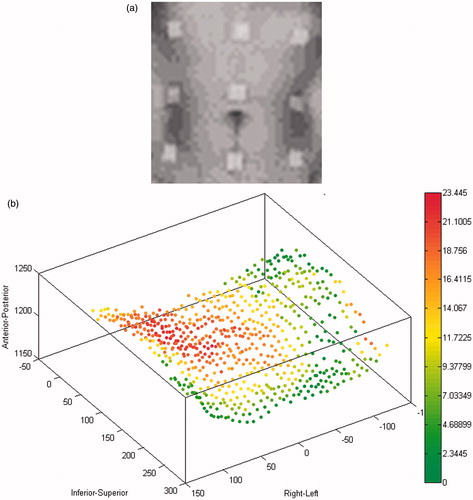The distance to the object can be computed as follows: where φ is the shift between the emitted and reflected light signals, and f is the frequency of the infrared (780 nm) cosine-shaped light signal. With the frequency set to 30 MHz, we can measure the distance to the objects for a 5 -m range area, which is sufficient to track respiratory motion with an accuracy of 1 cm. A previous study [13] showed the influence of warm-up time on the distance measurement stability. Measurements of the minimum relative variations of the mean values and standard deviations of the average range images were performed at a 3-m distance with a 100-ms integration time. Our approach was to acquire a 3D model including the attached markers. Figure 1 presents the intensity map of the abdomen and the point distances between the initial and target positions. The distance between the patient and the ToF sensor ranged between 1.0 and 1.5 m. Schaerer et al. [8] had previously used star-shaped markers, but we decided to use 15-mm square markers due to the lower resolution of our ToF intensity map.

Figure 1. (a) Zoomed intensity map for the ToF camera image of the abdomen with 9 square markers. (b) The color intensities describe the point distances between the initial and target positions.

Surface of respiratory motion registration

After acquiring the surface respiratory motion data, the next step is to perform registration. When the registration sets are in a point cloud configuration, the most popular approach is to use the Iterative Closest Point (ICP) algorithm. This algorithm was proposed independently by Besl and McKay [14] and Chen and Medioni [15]. The ICP is an iterative algorithm that consists of two steps. The first step involves the acquisition of the correspondence between the target and the source points, while the second step is to provide a transformation, calculated as follows: where T and S are the target and source sets of points, respectively, N_S is the number of source points equal to the target points, and Rot and Trans are the rotation and translation components, respectively, of the final transformation. The updated version of the final transformation in the current iteration is based on a closed-form solution of the mean square error problem [1]. The classical approach uses only one rigid or affine transformation for the whole data set. The literature contains a description of the disadvantages of the classical ICP approach [16]. These disadvantages can be summarized as follows:

• The problem of finding the global minimum of the cost function depends on an initial guess of the final transformation.

• The algorithm is sensitive to improper correspondence data.

• Long times are needed for computation. One of the most time-consuming operations is retrieving the correspondence data.

Due to these disadvantages, researchers have proposed various modifications:

• Registration only of subsets of points.

• An improved solution for the correspondence problem.

• Quantitative measurement of proper correspondence.

• Elimination of improper correspondence data.

• Modification of the computation of the minimum cost function.

We propose experiments that use some additional modifications:

• Registration of the entire sparse point cloud.

• Filtration of the potential correspondence data using the maximum normal angle condition.

• Use of the correspondence data in the directions of the normal and marker vectors.

• Use of a non-rigid ICP algorithm, similar to the Amberg modification.

The standard ICP approach cannot be used to track the surfaces of objects that change their shape over time, such as the human abdomen and chest during breathing, gesticulation or muscle flexion. In contrast to classical ICP, Amberg et al. [9] proposed the following equation: where E_d(X) is the distance between all target points and the transformed source points. X is not a single rotation or translation, but rather a collection of affine transformations for each point. E_s(X) is the stiffness regularization. The topology matrix is created based on the neighborhood of points to preserve the shape of the object during the iterations. We used a square matrix topology where every point has four neighbors. E_l(X) is a factor used for guiding the registration based on the known positions of landmarks in the source and target sets of points. The stiffness vector α influences the flexibility of the cloud shape.

The implemented non-rigid ICP algorithm consists of two iterative loops. In the outer loop, the stiffness factor α is gradually decreased with uniform steps, starting from higher values, which enables the recovery of an initial rigid global alignment, and proceeding to lower values, which allow for more localized deformations. For a given α value, the problem is solved iteratively in the inner loop. The condition for changing the stiffness vector is the threshold norm of the transformation difference from the adjoining iterations. The weighting factor β is used to decrease the importance of landmarks towards the end of the registration process. In our method, β is a constant equal to one. The above equation can be transformed into a system of linear equations, which are solved by computing the pseudo-inverse matrix.

Rigid registration paired-point method

To obtain rigid mapping between two Cartesian coordinate systems, data must include three or more sets of corresponding non-collinear points. Horn [17] proposed a closed-form solution based on a least-squares formulation. The optimal rotation Rot for the translation Trans matrices can be found using a singular value decomposition of where is the correlation matrix, S_i are points in the first Cartesian coordinate system, T_i are points in the second Cartesian coordinate system, σ_i is a non-negative singular value for the correlation matrix, and U and V are the orthonormal matrices: and where are the average values of the point coordinates in the first and second coordinate systems, respectively. This rigid registration approach was used for the initial registration of the point clouds before starting the normal shooting retrieving correspondence of the proposed non-rigid ICP algorithm.

Results and discussion

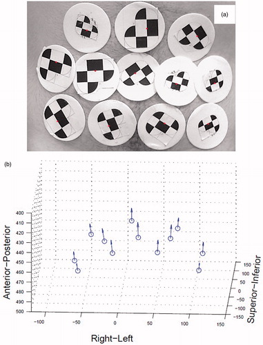
To track the twelve markers, the average number of frames per second was 5.4. The Claron system identifies points on the tracked object based on XPoints – the locations of the intersections of the white and black areas. The distance between two XPoints defines a vector. The two vectors that have different lengths and angles between 8° and 172° define the simplest marker. Each marker must have a unique shape. Based on these rules, we can propose markers for positions on the abdominal surface, as shown in Figure 2(a). The tracked markers highlight the differences in position between the opposite breathing phases (Figure 2b).

Figure 2. (a) Markers used on the abdomen in conjunction with the Micron Tracker Claron Hx 40 stereo camera. (b) Displacements of the markers between the opposite breathing phases (inhalation: blue points; exhalation: vectors).

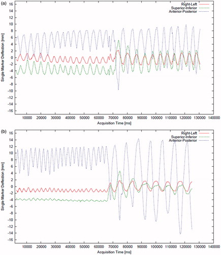
Figure 3 shows the multi-dimensional breathing signal extracted from the abdominal surface. Three spatial directions (i.e., superior-inferior, right-left and anterior-posterior) of the central marker (nearest to the navel) are presented for male and female patients. In the first minute, the patients breathe normally (shallow); in the second minute, they breathe deeply.

Figure 3. The time diagram for the skin central marker positions (near the navel) acquired with the Claron H×40 stereo camera for healthy male (a) and female (b) patients. The first minute shows shallow breathing; the second minute shows deep breathing. The position of the markers is spread in the right-left (RL), superior-inferior (SI) and anterior-posterior (AP) spatial directions.

The abdominal surface motions of the areas covered with the markers are presented in Table I. The average maximum for the movement of each of the five selected markers is presented for particular female and male subjects. We captured and registered the breathing motion while the patients were lying down using a Claron Hx40 camera mounted perpendicularly to the coronal plane.

Table I. Average maximum displacement of skin markers for male and female patients.

Marker	Shallow breathing [mm]			Deep breathing [mm]
position	A-P	R-L	S-I	A-P	R-L	S-I
Central	3.3	0.3	0.2	12.5	0.6	Irregular	Female
Right-lateral	3.6	0.2	0.8	10.7	0.7	2.4
Left-lateral	1.5	0.5	0.8	5.1	0.9	3.1
Top	3.4	0.6	0.4	11.8	1.7	1.2
Bottom	2.0	0.3	0.9	5.6	0.7	3.2
Central	3.0	0.6	1.5	7.0	2.2	3.0	Male
Right-lateral	2.2	0.3	0.2	6.5	0.8	0.6
Left-lateral	2.5	1.2	1.0	7.5	2.5	2.8
Top	4.1	1.1	0.6	11.2	2.3	0.9
Bottom	2.6	0.8	0.3	8.5	2.4	0.7

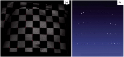
There are commercial systems that can be used for respiratory motion management (e.g., the PneumaCare system) that allow the registration of motion tracking data using chessboards displayed on white t-shirts that are registered with a stereo camera. Figure 4 shows our solution, which uses a chessboard projected on the chest and abdomen (Figure 4a) of the patient to reconstruct the cloud points (Figure 4b). This approach can be used to detect anomalies in the breathing motion; however, it causes displacement of the projected points on the thorax. Accurate tracking of the point correspondence on smooth surfaces is difficult for objects that change shape. The breathing process is remarkably patient-specific. The largest component of the skin marker movement is in the anterior-posterior projection. Deep breathing is sometimes irregular (see Figure 3), and for minimally invasive breathing motion compensation it is important to stabilize breathing. The main disadvantage of our approach is scalability, which needs to be improved to reconstruct the entire thorax and abdominal surface.

Figure 4. (a) Chessboard pattern projected on the abdomen to find the corners on the left and right images with sub-pixel accuracy using two monocular calibrated cameras and the Tsai algorithm. (b) Reconstructed corners of the chessboard for the Claron Hx 40 stereo camera.

Point cloud registration

The non-rigid ICP algorithm proposed by Amberg et al. [9] was tested with several modifications. This iterative algorithm performs iterations in two steps: finding correspondences between the source and target points and computing the affine transformations for each source point. If the second step is modified as proposed by Amberg et al., better results can be obtained. However, the correspondence problem remains critical for the final results. We therefore tested multiple approaches, searching for correspondences in the source and target point clouds using four methods:

• Classical searching based on the Euclidean distance between the closest points in the source and the target.

• Searching along the normal vectors of the source points, following the initial rigid registration method based on the Horn algorithm [17].

• Using static marker vector displacement, in which the marker vectors are calculated only once at the preliminary stage. The marker vectors are defined by the positions of specific markers in the source and target point clouds.

• Using dynamic marker vector displacement, in which marker vectors are calculated iteratively based on the constant positions of the nearest marker points in the matrix topology (Equation 5). Each iteratively transformed point is treated as a new origin for the dynamic marker vector.

We implemented the algorithm in C++ with an Eigen library. The point cloud area was limited to the central part of the abdomen, and the markers were chosen manually. We tested our approach on 9 subjects (3 females [F1-F3] and 6 males [M1-M6]) using point clouds captured in the opposite phases of breathing (inhalation and exhalation). Schaerer et al. [8] proposed the use of star markers, but due to the low resolution of our ToF intensity map, we used 15-mm square markers (Figure 1a).

The following global and local criteria were used for evaluation:

• Global measurements: average distances between the nearest source and target points, and average distances between correspondences.

• Local measurement – quality of correspondences: average correspondence assignment errors for the points nearest the markers.

Evaluation scores are presented for the different methods of finding the correspondences in Table II and Figure 5. In Table II, the data are presented for different subjects: F1-F3 and M1-M6. In Figure 5, cases M1 (green) and M5 (red) are shown because these data are specific with respect to the initial average distances between the nearest source and the target points (before registration). M5 has the nearest initial distance in the data set, and M1 has the furthest initial distance in the data set. For this reason, these cases are presented in detail in Figures 6 through 9.

Figure 5. (a, b) Global measurements: average distances between the nearest source and target points (a) and average distances between the correspondence values (b). (c) Local measurements (i.e., correctness of the correspondence average distances from the closest points to the markers for the source and target clouds) for different modifications of the ICP computing correspondence algorithm. E = Euclidean distance, NH = normal shooting with the initial rigid registration, SM = static marker vectors, and DM = dynamic marker vectors for the ToF camera.

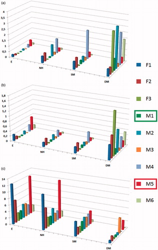
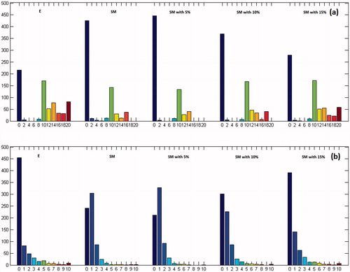
Figure 6. Distance map histogram (mm) (a) and correspondence map histogram (number of units) (b) for different modifications of the ICP computing correspondence algorithm for M5 (near). E = Euclidean distance, NH = normal shooting with the initial rigid registration, SM = static marker vectors, and DM = dynamic marker vectors for the ToF camera.

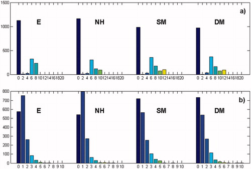
Table II. Scores for fitness (correspondence and surface distances and average marker errors) for four variants of the ICP algorithm: the Euclidean distance (E), normal vectors with the initial rigid registration (NH), static markers (SM) and dynamic markers (DM).

			After registration (after 100 iterations)
			Surface distance (mm)				Correspondence distance (mm)				Marker error (No. of units)
ID	No. of points	Initial	E	NH	SM	DM	E	NH	SM	DM	E	NH	SM	DM
F1	1152	5.83	0.21	0.6	0.69	0.63	0.26	0.18	0.25	0.58	12.42	10.81	4.45	0.76
F2	899	12.04	0.12	0.74	0.87	0.61	0.12	0.27	0.33	0.87	7.02	6.28	2.12	1.49
F3	506	25.16	0.03	0.03	0.06	3.43	0.04	0.03	0.03	1.7	2.57	2.9	1.86	0.44
M1	676	37.38	0.03	0.1	0.32	1.02	0.03	0.07	0.11	0.21	2.75	2.69	2.83	0.61
M2	506	19.84	0.14	1.04	0.51	3.56	0.14	0.22	0.15	0.88	4.3	4.63	3.6	0.72
M3	1892	5.21	0.004	0.21	0.28	0.28	0.04	0.07	0.1	0.1	4.05	2.61	3.11	4.69
M4	506	8.49	0.28	1.3	2.52	2.79	0.28	0.27	0.43	0.47	3.25	2.9	3.57	0
M5	1716	4.87	0.57	0.3	0.44	0.51	0.56	0.1	0.13	0.24	12.07	12.09	4.04	2.83
M6	528	10.76	0.16	0.15	0.09	1.94	0.16	0.07	0.06	0.53	2.25	1.89	0.75	0.09

Bold values indicate M1 and M5 had the furthest and nearest initial distances, respectively.

For M5 (the “near” case), the Euclidean distance computing correspondence works in a similar way to the other methods for finding correspondences. There are smaller white gaps in the transformed source point cloud (Figure 8, first picture in left column). White gaps mean that specific points overlap during the registration process. This phenomenon is also observed in the correspondence map histogram (Figure 6b). The groups with only one correspondence in the correspondence histogram for the Euclidean distance and the normal shooting (Figure 6b) are the largest because many points in the target clouds attract only one point from the source cloud. This situation is desirable in our case. The attraction of only one point is the only necessary condition for selecting a good correspondence, but it is not sufficient. We tested the quality of correspondence by selecting the nearest points to the markers in the source and target clouds and treating them as local patterns for the correct correspondence pairs. The calculation of the average correspondence assignment error for the nearest points for all markers is then performed. Using markers at the stage of choosing correspondences during registration improves the local measurement (the red bars in Figure 5c). The distance map histograms were similar for all methods used to find the correspondences (Figure 6a).

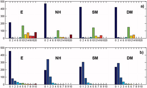
For M1 (the “far” case), the Euclidean distance does not work as well as the marker vectors. Although the average distances between the nearest source and target points have the smallest values, there are many gaps in the transformed source point cloud. This situation means that in many places the source point cloud locally coincides with a single point. The group with one correspondence in the correspondence histogram (Figure 7b) is the smallest for the Euclidean distance method. The average correspondence assignment error of the nearest points for all markers was similar between the Euclidean distance and normal shooting for the initial rigid registration and static marker vectors. Similar to the M5 case, the average correspondence assignment error was the smallest for the dynamic vector case. Generally, marker vector cases appear to work better for point clouds with larger initial average distances.

Figure 7. Distance map histogram (mm) (a) and correspondence map histogram (number of units) (b) for different modifications of the ICP computing correspondence algorithm for M1 (far). E = Euclidean distance, NH = normal shooting with the initial rigid registration, SM = static marker vectors (SM), and DM = dynamic marker vectors for the ToF camera.

To improve the retrieving correspondence using markers, we implemented a k-nearest neighbor method and a radius constraint to apply the marker information to not only every point in the cloud but also the nearest points to the markers. For points that are not near a marker, the Euclidean distance was used. Because the two proposed criteria are conceptually similar, we only present the radius constraint because it is more intuitive for users. We used the radius constraint percentage of the cloud width and the k-nearest criteria percentage of all points. The score results for three selected values (i.e., 5, 10 and 15%) were calculated. The results are presented in Table III and in Figures 10 and 11. For the most demanding criterion (5%), the results showed improvement (Figures 10 and 11).

Table III. Scores for fitness for the M1 and M5 static marker vectors with k-nearest and radius constraints.

			After registration (after 100 iterations)
			Surface distance (mm)				Correspondence distance (mm)				Marker error (No. of units)
ID	No. of points	Initial	SM	5%	10%	15%	SM	5%	10%	15%	SM	5%	10%	15%
M1 k-nearest	676	37.38	0.32	0.69	0.33	0.33	0.11	0.09	0.03	0.03	2.83	1.79	1.34	1.3
M5 k-nearest	1716	4.87	0.44	0.47	0.58	0.33	0.13	0.36	0.14	0.1	4.04	3.79	3.82	4.04
M1 radius constraint	676	37.38	0.32	0.07	0.05	0.02	0.11	0.07	0.05	0.03	2.83	1.33	1.14	1.79
M5 radius constraint	1716	4.87	0.44	0.05	0.43	0.4	0.13	0.06	0.45	0.36	4.04	3.6	4.31	3.79

Using the Claron Hx40 stereo camera and the projected chessboard pattern on the abdomen, a limited number of markers and points could be tracked. There are professional respiratory management systems that allow tracking of the entire abdominal and thoracic surface, but these systems are costly and require repeated calibration. We tested a similar approach for the opposite phases of the respiratory cycle, which, from the viewpoint of registration, appear to be the worst case, using a relatively inexpensive and readily available MESA SR4000 ToF sensor. This method allows us to increase the number of points that we track and does not require the implementation of advanced calibration procedures. The ToF camera is also small. In our approach, we focused on the registration area of the abdomen surface for different phases of the respiratory cycle and showed the possibility of using markers to find the correspondence using the non-rigid ICP algorithm. Clinical applications should still take into account the fact that the accuracy of the spatial reconstruction from the single points captured by the SR4000 camera is much lower than for the calibrated camera. This problem can be solved by reconstruction of the respiratory movement by finding the best-fit plane, for which the RMS error is less than 1 mm. The best-fit plane can be computed in real time [18]. Generally, we could follow the respiratory movement for different areas of different sizes, which is more universal than tracking only single markers.

For abdomen point clouds acquired from the opposite phases of the respiratory cycle, the registration process is still challenging. In our approach, we used less expensive equipment and focused on testing existing problems. The non-rigid ICP algorithm provided an average residual distance of 0.93 mm (Euclidean distance not included). Further analysis of the registration accuracy focused on solving the correspondence problem. Four methods for solving this problem were tested: the Euclidean distance treated as a base line; normal shooting with initial rigid registration based on the Horn algorithm; static marker vectors (computing only one at the beginning of the registration process); and dynamic marker vectors (computing vectors for every iteration). Because directly measuring the quality of correspondences is difficult, an observation method was proposed involving a few steps. The correspondence map (right column of Figures 8 and 9) showed the spatial distribution of the features and the number of correspondences assigned to each target point (the desirable value is 1). Comparing correspondence maps globally for different cases is simple using a correspondence map histogram (Figures 6b, 7b, 10b and 11b). The average correspondence assignment errors for the points nearest the markers enable the measurement of the quality of the correspondence points from the cloud, which are nearest to the markers.

Figure 8. The 95th percentile distance map (mm) (left column) and the correspondence map (number of units) (right column) for different modifications of the ICP computing correspondence algorithm for M5 (near). E = Euclidean distance, NH = normal shooting with the initial rigid registration, SM = static marker vectors, and DM = dynamic marker vectors for the ToF camera.

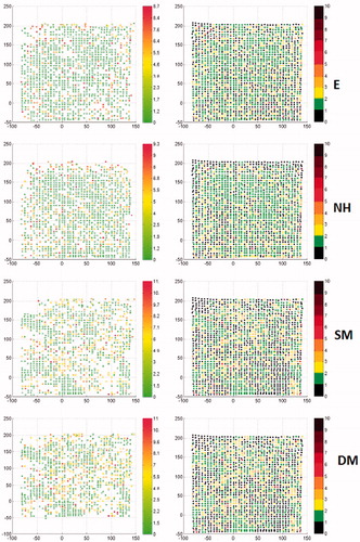
Figure 9. The 95th percentile distance map (mm) (left column) and the correspondence map (number of units) (right column) for different modifications of the ICP computing correspondence algorithm for M1 (far). E = Euclidean distance, NH = normal shooting with the initial rigid registration, SM = static marker vectors (SM), and DM = dynamic marker vectors for the ToF camera.

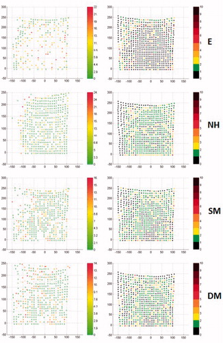
Figure 10. Distance map histogram (mm) (a) and correspondence map histogram (number of units) (b) for different modifications of the ICP computing correspondence algorithm for M5 (near): Static marker vector and static marker vector with 5%, 10% and 15% radius constraints for the ToF camera.

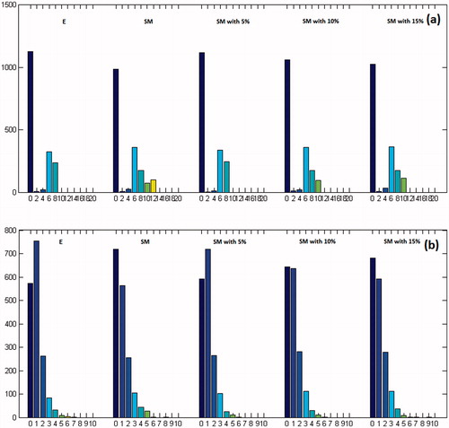
Figure 11. Distance map histogram (mm) (a) and correspondence map histogram (number of units) (b) for different modifications of the ICP computing correspondence algorithm for M1 (far): Static marker vector (SM) and static marker vector with 5%, 10% and 15% radius constraints for the ToF camera.

The average initial distance of the point clouds achieved for the opposite breathing phases was used to divide our analysis into two groups. For the “near” cloud group, the stiffness vector was constant for almost every iteration of the non-rigid ICP. The Euclidean distances for this group were sufficient, which is in accordance with the results of Schaerer et al. [8]. In contrast to the “near” clouds, the “far” clouds had stiffness vectors that changed for some iterations. The Euclidean distances for the far cloud group were not sufficient, and there were many gaps present in the registered source clouds. To address this issue, we proposed the use of static and dynamic marker vectors. If the markers are used not only in computing the transformation step but also in computing the correspondence step for each iteration, the correspondence assignment error for the points nearest to the markers decreases from 5.4 to 2.1 for confused neighbors. The normal shooting approach was also evaluated, but the results were worse than for other cases. However, a combination of normal shooting and initial rigid registration improved the results significantly. For medical applications based on ToF sensors, simplifying the registration process is desirable; therefore, a synchronization mechanism for acquiring data should be considered. Our results may also be used in various entertainment and industrial applications for which point clouds must be registered but high-cost equipment is not available. Some shape measurements could be used as distinguishing criteria for “near” and “far” clouds.

Different approaches have been evaluated to track abdominal respiratory motions. Generally, these tracking results can be used to prepare respiratory motion models, which are necessary for radiotherapy, when the pathological tissue is usually located inside the body and different surrogate signals are used to create respiratory motion models [19]. The surrogate breathing information from a few external markers is not sufficient to build a reliable model in every case, and internal breathing gating, which can be more useful, cannot be used in every medical application because it increases invasiveness. Thus, there is interest in acquiring more sophisticated information on breathing during interventions to obtain better external gating (e.g., Hostettler et al. [20] proposed an estimation of the visceral position based on abdominal and thorax surface registration). The development of relatively inexpensive ToF sensors provides hope for methods such as non-rigid ICP, which has been adopted to build breathing motion models. Our pilot study confirms the possibility of using modified non-rigid ICP algorithms and ToF sensor data as inputs to build such models.

Declaration of interest

The authors would like to acknowledge financial support from The National Center for Research and Development in Poland, grant no. LIDER/03/47/L-1/NCBiR/2010: “Development of a planning system and computer-aided minimally invasive surgery for hepatic and metastatic liver carcinoma localization, diagnosis and destruction”.

References

- Hawkes D, Barratt D, Carter T, McClelland J, Crum B. Nonrigid Registration. In: Peters T, Cleary K, editors: Image-Guided Interventions: Technology and Applications. New York: Springer, 2008. pp. 193–218
- Spinczyk D, Karwan A, Rudnicki J, Wróblewski T. 2012. Stereoscopic liver surface reconstruction. Wideochir Inne Tech Malo Inwazyjne 7(3):181–7
- Borgert J, Krüger S, Timinger H, et al. 2006. Respiratory motion compensation with tracked internal and external sensors during CT-guided procedures. Comput Aided Surg 11(3):119–25
- Maier-Hein L, Tekbas A, Franz AM, et al. 2008. On combining internal and external fiducials for liver motion compensation. Comput Aided Surg 13(6):369–76
- Case Study: A Novel Way of Analysing Breathing Pattern. Manufacturer's website: http://www.pneumacare.com/Clinical-Data/respiratory/Case-Studies.aspx
- Ford E, Mageras G, Yorke E, et al. 2002. Evaluation of respiratory movement during gated radiotherapy using film and electronic portal imaging. Int J Radiat Oncol Biol Phys 52(2):522–31
- Meeks S, Tomé W, Willoughby T, et al. 2005. Optically guided patient positioning techniques. Semin Radiat Oncol 15(3): 192–201
- Schaerer J, Fassi A, Riboldi M, et al. 2012. Multi-dimensional respiratory motion tracking from markerless optical surface imaging based on deformable mesh registration. Phys Med Biol 57(2):357–73
- Amberg B, Romdhani S, Vetter T. 2007. Optimal step nonrigid ICP algorithms for surface registration. Proceedings of the IEEE Computer Society Conference on Computer Vision and Pattern Recognition (CVPR 2007), Minneapolis, MN, June 2007. pp. 1–8
- Nicolau SA, Goffin L, Graebling P, et al. 2008. A structured light system to guide percutaneous punctures in interventional radiology. Proceedings of the SPIE Conference on Optical and Digital Image Processing, Strasbourg, France, April 2008. Proc SPIE 7000:700016
- Hartley RI, Zisserman A. 2004. Multiple View Geometry in Computer Vision. 2nd edn. Cambridge, UK: Cambridge University Press. pp. 262–76
- Chiabrando F, Piatti D, Rinaudo. 2010. Sr-4000 ToF Camera: Further experimental tests and first applications to metric surveys. Proceedings of the International Society for Photogrammetry and Remote Sensing Commission V Symposium, Newcastle upon Tyne, UK, June 2010. International Archives of Photogrammetry, Remote Sensing and Spatial Information Sciences 38(5):149–54
- Chiabrando F, Chiabrando R, Piatti D, Rinaudo F. 2009. Sensors for 3D imaging: Metric evaluation and calibration of a CCD/CMOS time-of-flight camera. J Sensors 9(12):10080–96
- Besl PJ, McKay ND. 1992. A method for registration of 3D shapes. Pattern Anal Machine Intell 14(2):239–56
- Chen Y, Medioni G. 1992. Object modeling by registration of multiple range images. Image Vision Comput 10(3):145–55
- Rusinkiewicz S, Levoy M. 2001. Efficient variants of the ICP algorithm. Proceedings of the 3rd International Conference on 3-D Digital Imaging and Modeling, Quebec City, Canada, May 28-June 1, 2001. pp. 145–52
- Horn B. 1987. Closed form solution of absolute orientation using unit quaternions. J Opt Soc Am A 4(4):692–42
- Schaller C, Penne J, Hornegger J. 2008. Time-of-flight sensor for respiratory motion gating. Med Phys 35(7):3090–3
- McClelland JR, Hawkes DJ, Schaeffter T, King AP. 2013. Respiratory motion models: a review. Med Image Anal 17(1):19–42
- Hostettler A, Nicolau SA, Rémond Y, et al. 2010. A real-time predictive simulation of abdominal viscera positions during quiet free breathing. Prog Biophys Mol Biol 103(2–3):169–84