Exploring QSARs of the interaction of flavonoids with GABA (A) receptor using MLR, ANN and SVM techniques

Abstract

Quantitative Structure–Activity Relationship (QSAR) models for binding affinity constants (log K_i) of 78 flavonoid ligands towards the benzodiazepine site of GABA (A) receptor complex were calculated using the machine learning methods: artificial neural network (ANN) and support vector machine (SVM) techniques. The models obtained were compared with those obtained using multiple linear regression (MLR) analysis. The descriptor selection and model building were performed with 10-fold cross-validation using the training data set. The SVM and MLR coefficient of determination values are 0.944 and 0.879, respectively, for the training set and are higher than those of ANN models. Though the SVM model shows improvement of training set fitting, the ANN model was superior to SVM and MLR in predicting the test set. Randomization test is employed to check the suitability of the models

• ANN
• flavanoids
• GABA (A) receptor
• machine learning methods
• SVM

Introduction

Flavonoids are a group of low molecular weight plant1,2 products, based on the parent compound, flavone (2-phenylchromone) and have shown potential for application in a diversity of pharmacological targets. Flavonoids are responsible for many of the shining colors of fruits and vegetables and are important constituents of green tea, coffee, chocolate, red wine and many herbal preparations. The lipophilicity of some flavonoids allows them to cross the blood–brain barrier3, therefore, it is likely that diet-derived flavonoids are found in brain.

Many flavonoids are polyphenolic and are thus powerfully antioxidant4. They have a broad diversity of biological activities and are being considered intensively as anticancer agents5 for their special effects on the vascular system6.

In addition, flavonoids have confirmed anxiolytic, sedative and anticonvulsant activities. Even though their actions in the central nervous system take place through a diversity of interactions with diverse receptors and signalling pathways, it is supposed that some of these special effects are mediated by ionotropic GABA, especially GABA (A) receptors. Several attempts have been made to make synthetic flavones derivatives with higher affinities for the GABA (A) receptor7–12.

Quantitative structure--activity relationship (QSAR) studies were conducted in order to build models for inhibition of GABA (A) receptor that could serve as a lead for the rational design of further potent and selective inhibition having the flavones backbone. An attempt was made by Duchowiz and co workers13. They have proposed the best linear model for a set of 70 flavones and found that the best model involves four correlating descriptors with statistical quality given by R²= 0.7174. The authors of this study performed recently QSAR studies on flavoniods, for example, Khadikar et al.14 published 2D-QSAR models for binding affinity constants of 78 flavanoid ligands towards the benzodiazepine site of GABA (A) receptor complex were estimated using the PRECLAV (Property-Evaluation by Class Variables) program. The best MLR equation with nine PRECLAV descriptors has R²= 0.8098. Two more QSAR studies were conducted in which flavonoids are being tested as specific inhibitors of protein tyrosine kinase (PTK) by Deeb. In the first one15, the flip regression procedure has been applied to 54 flavonoid analogues. It is shown that the orientation of nodes in their occupied π orbitals, and also the energies of these orbitals, explain a further large portion of the variance in their inhibitory activity. In the second one16, an optimal approach for variable selection in Counter-Propagation Neural Networks (CPNN) were conducted in modeling protein tyrosine kinase inhibitory of 105 flavonoids using Substituent Electronic Descriptors (SED). The results indicated that CPNN is a useful classifier tool in pattern recognition of data sets with discrete activity (i.e. active and non-active) in combination with variable selection procedure.

In this contribution, we are trying to build new QSAR models for the interaction of 78 flavonoids with GABA (A) receptor using machine learning methods such as ANN and SVM. These models will serve as a tool for designing new drugs.

Materials and methods

Data set

The data set used in this study consists of 78 flavoniods, presented in Table 1, together with their log K_i(μM) values13. The chemical structures were generated with HyperChem (version 7.5; Hypercube, Inc., Gainesville, FL)17. AM1 method18 was applied to optimize the molecular structure of the compounds. No molecular symmetry constraint was applied; rather full optimization of all bond lengths and angles was carried out. All calculations were carried out at the restricted Hartree–Fock level with no configuration interaction. The molecular structures were optimized using the Polak–Ribiere algorithm until the root mean square gradient was 0.01 Kcal/mol. Geometry optimization was run multiple times with different starting points for each molecule, and the lowest energy conformation was considered for the calculation of electronic properties.

Table 1. List of 78 flavoniods and their observed, estimated log K_i values (MLR) with their residuals.

Compd. No.	Compound	Obs. log Ki	Est. log Ki MLR	Residual MLR
Training set
3	6-Chloro-4′-methoxyflavonc	0.097	0.367	−0.270
4	6-Bromo-4′-methoxyflavone	0.322	0.449	−0.127
6	6-Bromo-2′-fluoroflavone	−0.424	0.186	−0.610
7	6,3′-Difluoroflavone	−0.036	0.186	−0.222
8	6-Chloro-3′-fluoroflavone	−0.932	−0.734	−0.198
9	6-Bromo-3′-fluoroflavone	−1.377	−1.231	−0.146
10	4′-Fluoroflavonc	0.556	0.304	0.252
12	6-Chloro-4′-fluoroflavone	−0.742	−0.901	0.159
13	3′-Chloroflavone	−0.212	−0.262	0.050
14	6,3′-Dichloroflavone	−1.638	−1.367	−0.271
15	3′-Bromoflavone	−0.384	−0.553	0.169
16	6-Fluoro-3′-bromoflavone	−0.627	−0.688	0.061
17	6-Chloro-3′-bromoflavone	−1.638	−1.673	0.035
19	6-Bromo-4′-nitroflavone	−0.699	−0.382	−0.317
20	6-Bromoflavone	−1.155	−1.379	0.224
21	6-Chloroflavone	−0.785	−0.806	0.021
23	6-Methoxyllavone	−0.066	0.412	−0.478
24	6-Fluoroflavone	0.653	0.176	0.477
25	6-Bromo-3′-nitroflavone	−3.000	−2.418	−0.582
26	6-Methyl-3′-nitroflavone	−2.252	−2.131	−0.121
27	6-Chloro-3′-nitroflavone	−2.097	−2.285	0.188
29	6-Fluoro-3′-nitroflavone	−0.745	−0.911	0.166
30	3′-Nitroflavonc	−0.545	−0.582	0.037
31	6-Methyl-3′-bromoflavone	−1.886	−1.523	−0.363
32	6-Nitro-3′-bromoflavone	−1.602	−1.658	0.056
33	6-Hydroxy-3′-bromoflavone	0.000	−0.539	0.539
34	6-Methoxy-3′-bromoflavone	0.000	−0.066	0.066
35	6-3′-Dimethylflavone	−0.682	−0.634	−0.048
36	3′-Methylflavone	1.000	0.332	0.668
37	5,2′-Dihydroxy-6,7,8,6′-tetramethoxy flavone	−0.444	0.061	−0.505
38	5,7,2′-Trihydroxy-6,8-dimethoxyflavone	−2.215	−1.650	−0.565
39	2′-Hydroxy-a-napthoflavone	−1.569	−1.452	−0.117
42	5,7,2′-Trihydroxyflavone	−1.125	−0.354	−0.771
44	5,7-Dihydroxy-6,8-dimethoxyflavone	−0.699	−1.776	1.077
47	5,7-Dihydroxy-8-methoxyflavone	0.182	0.037	0.145
48	6-F-Hydroxyflavone	0.422	0.230	0.192
49	7-Hydroxyflavone	0.623	0.561	0.062
50	5,6,7-Trihydroxyflavone	0.747	1.264	−0.517
51	6-Hydroxy-2′-mcthoxytlavone	0.976	1.163	−0.187
54	Flavone	0.000	0.416	−0.416
55	5,7-Dihydroxyflavone	0.477	0.828	−0.351
56	5,3′,4′-Trihydroxy-6,7-dimethoxyflavone	2.301	1.649	0.652
57	5,4′-Dihydroxy-6,7-dimcthoxyflavone	1.362	1.216	0.146
59	5,7-Dihydroxy-2′-chloroflavone	0.903	0.519	0.384
61	5,7-Dihydroxy-6,8-dibromoflavone	−0.155	0.158	−0.313
62	5,7,4′-Trihydroxyflavone	0.602	1.059	−0.457
63	3,5,7,4′-Tetrahydroxytlavone	1.969	1.356	0.613
64	5-Hydroxy-7-methoxyllavone	1.699	1.448	0.251
66	6-Fluoro,3′-hydroxyflavone	0.400	0.162	0.238
67	6-Chloro,3′-hydroxyflavone	−0.070	−0.337	0.267
69	6-Bromo-2′-nitrotlavone	−0.680	−1.359	0.679
70	6-Nitro-4′-bromollavone	−1.600	−1.829	0.229
73	3′-Fluoroflavone	0.550	0.386	0.164
74	6-Bromo-4′-fluoroflavone	−0.939	−1.470	0.531
75	6-Fluoro-3′-chlorollavone	−0.701	−0.421	−0.280
76	6-Bromo-3′-chlorollavone	−1.770	−1.637	−0.133
77	6-Methylflavone	−0.903	−0.853	−0.050
78	6-Bromo-3′-methylflavone	−0.812	−0.428	−0.384
Test set
1	6-F-luoro-3′-methoxyflavone	0.398	0.843	−0.445
2	6-Bromo-3′-mcthoxyflavone	−0.215	0.247	−0.462
5	6-Chloro-2′-fluoroflavone	−0.380	−1.714	1.334
11	6,4′-Difluoroflavone	0.398	0.025	0.373
18	6,3′-Dibromollavone	−1.721	−2.01	0.289
22	6-Nitroflavone	−0.561	−0.288	−0.273
28	6-3′-Dinitroflavone	−1.585	−1.592	0.007
40	6,2′-Dihydroxyflavone	−1.469	−0.422	−1.047
41	5,7,2′-Trihydroxy-b.-methoxyflavone	−1.420	−0.45	−0.970
43	2′-Hydroxyflavone	−0.678	−1.016	0.338
45	7,2′-Dihydroxyflavone	−0.252	−0.234	−0.018
46	5,7-Dihydroxy-6-methoxyflavone	−0.051	−0.015	0.066
52	2′-Methoxyflavone	1.508	1.427	0.081
53	2′-Amino-6-methoxyflavone	0.544	0.191	0.353
58	5,7,4′-Trihydroxy-6-mcthoxyflavone	0.000	0.056	−0.056
60	5,7-Dihydroxy-2′-fluoroflavone	0.903	1.099	−0.196
65	5,7-Dihydroxy-6,8-diiodollavone	0.000	−0.281	0.281
68	6-Bromo,3′-hydroxyflavone	−0.220	−0.926	0.706
71	3′-Methoxyflavone	0.380	0.918	−0.538
72	6-Chloro-3′-methoxyflavone	−0.072	0.401	−0.473

Molecular descriptors

In this study, a pool of descriptors classified into 18 different groups was calculated using Dragon software (version 6.0, Dragon Talete srl; http://www.talete.mi.it/). The constant or nearly constant descriptors for all the 78 compounds were discarded from further analysis. These groups of descriptors are: molecular walk counts, Galves topological charge indices, Randic molecular profiles, aromaticity indices, functional groups, atom-centered fragments, constitutional, charge, RDF, WHIM, topological, BUCT, geometrical, 3D-MoRSE, GETAWAY and 2D descriptors. Furthermore, chemical descriptors such as HOMO energies (Highest occupied molecular orbital), LUMO (Lowest unoccupied molecular orbital) energies and polarizability were calculated using HyperChem software. Depending on the HOMO and LUMO values, electrophylicity, electronegativity, hardness, and softness descriptors were calculated. Other descriptors such as surface area approximate, surface area grid, volume, mass, polarizability, hydration energy, octanol--water partition coefficient (log P), and refractivity were calculated also as a separate group. By discarding the highly inter-correlated (r > 0.95) descriptors, the total number of descriptors were reduced. These descriptors were used for MLR, ANN and SVM analysis.

Selection of training set and test set for external validation

In QSAR studies a training set is used for the development of the models, and a test set, which was never incorporated through their development, used to validate the external predictivity of the models19,20, The data set was split into training and test sets21 using the STATISTICA DATAMINER software ver. 10 (StatSoft, Inc., Tulsa, OK) by random sampling technique in which 75% (58 compounds) of the data was taken as training set and the remaining 25% (20 compounds) as test set for MLR, ANN and SVM analysis.

Descriptor selection and linear model generation

To generate a stable model, appropriate descriptors should be selected in QSAR study. We used a bi-directional search method which is a combination of forward and backward search, and then the selected descriptors are evaluated on the training set for modeling of log K_i values. Then the selected descriptors set was subjected to multiple linear regression analysis to produce a linear model.

Validation techniques and model performance evaluation

For MLR, we used internal cross validation and for ANN and SVM techniques we used a 10-fold cross validation technique. This procedure divides the data set into 10-folds or groups and creates the model using nine of the sets and tests it on the remaining group. This procedure is repeated until each of the 10 groups has served as a test group. The error estimates, root mean square error (RMSE) and mean absolute error (MAE) are calculated and then averaged.

In this study, the 58 training data set was randomly divided into 10 groups and the model was trained on 9 groups and the remaining one group is used for testing each time. The error measures RMSE and MAE are used to evaluate the predictive performance of the models.

Artificial neural network

Artificial neural networks (ANNs) are computer-based models in which a number of nodes, also called neurons, are interconnected by links forming netlike structure “layers”. A variable value is assigned to every neuron. There are three kinds of neurons: (1) the input neurons which receive their values from independent variables and constitute the input layer, (2) the hidden neurons which collect values from other neurons, giving a result that is passed to a successor neuron, (3) the output neurons which take values from other units and correspond to different dependent variables, forming the output layer. In this sense, network architecture is commonly represented as I–H–O, where I, H, and O are the number of neurons in the input, hidden, and output layers, respectively.

The weights are links between units that condition the values assigned to the neurons. The weights are adjusted through a training process in order to minimize network error. For this, a non-linear transfer function relates the input parameters with the outputs. Commonly neural networks are adjusted, or trained, so that a particular input leads to a specific target output. The model development in ANN and the network architecture is fully described by us and others22,23. The training set was used to optimize the network performance. The regression between the network output and the observed binding affinity was calculated for the training as well as the test sets individually. The training function “Tanh” was used to train the network. To find models with lower errors, the ANN algorithm was run many times, with different geometry and initial weights each time.

Support vector machine

Support vector machine (SVM) can be applied to regression by the introduction of an alternative loss function. In support vector regression (SVR), the basic idea is to map the data X into a higher-dimensional feature space F via a nonlinear mapping Φ and then to do linear regression in this space. Therefore, regression approximation addresses the problem of estimating a function based on a given data set ( contains independent variables, y_i contains dependent variables and N is the total number of data patterns). SVM approximates the function in the following form: where w is weight vector, is the set of mappings of input features, and b are the slope and offset of the regression function, respectively.

In the current work, the Gaussian radial basis function (RBF) kernel was used as a kernel function, k(x_i,x_j) = exp (−(||xⁱ− x_j||²)/2σ2), where σ² is the width of the Gaussian function, so the C and σ which are the relative weights of the regression error and the kernel parameter of the RBF kernel should be optimized by the user, to obtain the support vector. The parameters of SVMR were optimized by systemically changing their values in the training step and calculating the RMSE and accuracy of the model using 10-fold cross-validation. The optimized values of C, σ2, and ε (ε is a precision parameter representing the radius of the tube located around the regression function f(x)) were 140, 0.1, and 0.03, respectively, obtained based on minimum RMSE and maximum accuracy of the model. This method was discussed in details by Deeb et al.24.

Results and discussion

Linear model (MLR model)

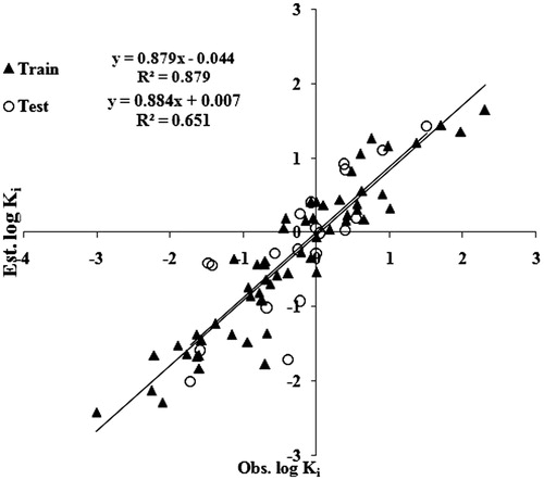
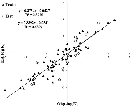
As mentioned in the descriptor selection section “Successive regression” – with multiple linear regression as the target, learning algorithm estimated a subset of 13 descriptors. The reduced descriptor subset is then used for linear model building using a multiple linear regression analysis. The best resulted linear model selected 10 relevant descriptors to give a stable model with R²= 0.879. The correlation matrix for the selected descriptors is given in Table S1 in the supplementary materials. Figure 1 shows the correlation between observed and estimated log K_i values for the best linear model obtained from training set. The resulting model equation with 10 correlating descriptors along with their cross-validated parameters is shown below. These 10 descriptors were further used in ANN and SVM techniques.

Figure 1. Correlation between observed and estimated log K_i for the best MLR model.

Here N is the number of compounds, R²= Squared correlation coefficient,  = Adjusted R², Se = Standard Error of estimate, F = Fisher’s Ratio, and Q = Pogliani quality factor. PRESS =predicted residual sum of squares, SSY = sum of squares of response value. PRESS/SSY = a value smaller than 0.4 indicates reasonable QSAR model,  = cross-validated correlation coefficient, S_PRESS = uncertainty of prediction, PSE = Predictive Square Errors, RMSE = root mean square error, MAE = mean absolute error. The above-reported model has further been used to predict the log K_i values of the remaining 20 compounds which are used as test set. Such predicted values are also recorded in Table 1. The predicted R² value for the test set has been obtained by plotting a graph between the observed and estimated log K_i values for the compounds and is demonstrated in Figure 1. The comes out to be 0.651 confirming that the proposed model is meaningful. The RMSE and MAE values for the test set are 0.145 and 0.033, respectively.

The ratio PRESS/SSY can be used to calculate approximate confidence intervals of the prediction of new compounds. To be a reasonable and significant QSAR model, the ratio PRESS/SSY should be less than 0.4 (PRESS/SSY < 0.4) and the value of this ratio smaller than 0.1 indicates an excellent model. A close look to the above model shows that the model has the PRESS/SSY ratio nearer to 0.1, indicating that the proposed model is having best predicting capacity. is the cross-validated squared correlation coefficient. The highest value (0.862) for the above model confirms our findings. The two important cross-validation parameters, uncertainty in prediction (S_PRESS) and predictive squared error (PSE), were also calculated. For this model, the value of SSY is high, whereas the values of PRESS, PRESS/SSY, S_PRESS, and PSE are low, indicating good model.

A brief description of the selected descriptors in the MLR model is given in Table 2. We notice from the above equation that the most contribution to the binding affinity come from the two descriptors JGI9 (Mean topological charge index of order 9), it is among the topological charge indices, and MSD (Mean Square Index (Balaban), it is among the topological descriptors.

Table 2. A brief description of the selected descriptors in the MLR model.

No.	Symbol	Descriptor type	Meaning
1	MSD	Topological	Mean Square Index (Balaban)
2	PJI2	Topological	2D Petitjean Shape Index
3	IVDE	Information	Mean information content on the vertex degree equality
4	MATS8v	2D-Autocorrelation	Moran auto correlation –lag 8/weighted by atomic van der waals volumes
5	MATS2e	2D-Autocorrelation	Moran auto correlation –lag 2/weighted by atomic Sandersons electronegativities
6	GATS8e	2D-Autocorrelation	Geary auto correlation –lag 8/weighted by atomic Sandersons electronegativities
7	JGI9	Topological charge	Mean topological charge index of order 9
8	L/Bw	WHIM	length to breadth ratio by WHIM
9	R4e+	GETAWAY	R maximal auto correlation of lag 4/weighted by atomic sanderson electronegativities
10	nRORPh	Functional group counts	number of ethers

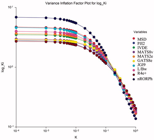
The most appropriate model given above is subjected to Ridge regression for investigating the existence or otherwise of any colinearity defect. The Ridge parameters, namely, VIF (variance inflation factor), T (Tolerance), λ_i (Eigen values), and k (Condition number), have been calculated and presented in Table S2 in the supplementary materials. We observed that VIF (variance inflation factor) values are much smaller than the allowed range of 10. Also, that condition number for the correlating parameters all are much lower than 100 and the tolerance are <1. These observations therefore, suggest that no co-linearity defect is present in the proposed model. The ridge trace and variance inflation factor plot for the obtained best model is reported in Figures 2 and 3, respectively. These figures suggest that no colinearity defect is present in the proposed model The symbol k on x-axis represents the condition number. Ridge regression is done with the help NCSS software.

Figure 2. Ridge trace for the 10-variable model. (Color version available online at: informahealthcare.com/enz)

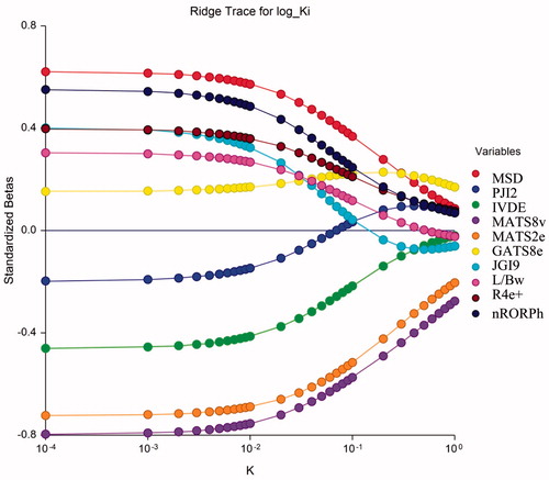
Figure 3. VIF plot for the 10 variable model. (Color version available online at: informahealthcare.com/enz)

ANN results

The initial architecture of the ANN selected was 10 neurons in the input layer and four neurons in the hidden layer selected by the auto build function and one output neurons. The input neurons correspond to 10 selected descriptors of the best MLR model. The ideal value of learning rate h and momentum m was determined by varying their values from 0.01 to 1.0, the combination of h = 0.1 and m = 0.2 which gives the lowest RMSE was selected. The optimization was done with 10-fold cross validation.

With the above-selected parameters the number of neurons in the hidden layer was optimized by varying from 1 to 10, it is worthy to mention that the initial value of 4 selected was optimal. When the entire training data is trained in the network with the optimized parameters, it gives an R²= 0.8775, RMSE = 0.03, and MAE = 0.04.

A plot of the observed and predicted values of log K_i of the training as well as the test data using the ANN model is shown Figure 4. Using the trained network, the test set was used for prediction and gives R²= 0.688, RMSE = 0.04, and MAE = 0.009.

Figure 4. Correlation between observed and predicted log K_i for the best ANN model of the training and test sets.

SVM results

The optimization of SVM parameters was performed by systematically varying the parameter values in the training step using 10-fold cross-validation and calculating the RMSE of the model. The parameter value which gives the lowest RMSE was selected. The regularization parameter C controls the tradeoff between maximizing the margin and minimizing the training error. If the value of C is too small, then insufficient stress will be placed on fitting the training data. To make the learning process stable, a large value should be set up for C initially. We kept the value of C as 100 initially and optimized kernel parameter γ and tube size ε.

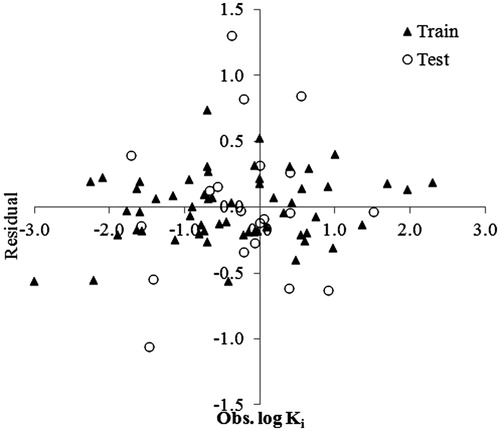
The RBF kernel parameter γ controls the amplitude of the Gaussian function, and further effect the generalization ability of SVM. The parameter ε of e-insensitive loss function is referred to as the tube size, and it is defined as the approximation accuracy placed on the training data points. The value of ε also decides the number of support vectors: higher the value, fewer support vectors are selected. In order to find the optimum values of two parameters (γ and ε), the 10-fold cross-validation based on the training set was performed and values giving the lowest RMSE was selected. Using the selected parameters (γ = 0.1, ε = 0.03, C = 140), final training was run on entire training set and the log K_i values were predicted. The plot of predicted versus experimental log K_i for the training and test sets based on this model is shown in Figure 5, while Figure 6 shows their residuals against the observed log K_i values. As we can see from the figure, the points are distributed (scattered) around the zero, which means that we did not have outliers. The statistical parameters of this model are RMSE = 0.03, R²= 0.944, and MAE = 0.04 for the training set. This SVM model is used to predict log K_i values of the test data set. The prediction statistics of SVM model is, RMSE = 0.07, R²= 0.678, and MAE = 0.001. Table S3 in the supplementary materials shows the predicted log K_i values by ANN and SVM for the training as well as for the test sets.

Figure 5. Correlation between observed and predicted log K_i for the best SVM model of the training and test sets.

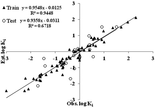
Figure 6. Residue against observed log K_i for the SVM model.

From the statistical parameters of the results obtained from the studied models for training and test set compounds, we see that the error estimates used for model performance evaluation, RMSE, and MAE were lower for nonlinear models (SVM, ANN) generated by the machine learning methods. The correlation coefficients (R) given by SVM and ANN models is also higher. This demonstrates that the performances of nonlinear models are better than that of a linear MLR model. The comparison of performance of the nonlinear models demonstrates that the SVM model predicts the binding affinity of the compounds more accurately than the ANN model for the training set. This is evident from a lower RMSE and a higher R value, while the test set prediction is better with the ANN model.

For judging the quality of the aforementioned model, metrics method has been applied25. According to above metrics25, for an acceptable QSAR model, the value of “Average ” should be >0.5, “” should be <0.2 and slopes26 should be 0.85 ≤ k ≤ 1.15 or 0.85 ≤ k¹≤ 1.15. Squared correlation coefficient values between the observed and predicted values of the compounds with intercept (r²) and without intercept () are calculated for the determination of . Changing the axes gives the value of , which will be used to calculate the . The parameter “k” indicates the slope of the observed and predicted values plot while “k¹” indicates the slope when changing the axes. Presently two different variants of this parameter, and , slopes k and k1 were calculated for both the training (internal validation) and test (external validation) sets in addition to the total dataset (overall validation). The , , k and k1 values for all the training, test and overall datasets (MLR, ANN, and SVM) are reported in Table S4 in the supplementary materials. A close observation of this table clearly indicates that all the values obtained from the metrics and slopes are within the range and judging the quality of the model.

Randomization test is performed to investigate the probability of chance correlation for the optimal models. In this test, the dependent variable vector (log K_i) is randomly shuffled and new QSAR models are explored using the original independent feature matrix (descriptors). After performing the randomization test, the results indicate that the coefficient of determination obtained by chance is low while the RMSE values are high. This indicates that the models obtained in this study are better than those obtained by chance.

Comparison with other QSAR studies

Duchowiz and co workers13 proposed the best linear model for a set of 70 flavones and found that the best model involves four correlating descriptors with statistical quality given by R²= 0.7174. It is interesting to compare our results with the results of Khadikar et al.14. They developed best MLR equation with nine PRECLAV descriptors (Property-Evaluation by Class Variables) having the R²= 0.8098 but they deleted seven compounds as outliers from the original set. Our model is with 10 correlating parameters having the R²= 0.879 in training set and  = 0.651 in test case. Our MLR model is better than the previously reported one by Khadikar et al. In addition to that, we have also applied ANN and SVM techniques in which the statistical parameters are better, especially with SVM method.

Conclusions

A comparison of results from the model performance demonstrates that the SVM model predicts the binding affinity of the compounds more accurately than ANN and MLR models for the train dataset, while for test set prediction, ANN model was better. The proposed models could identify and provide some important information which is responsible for drug-binding affinity. Employed randomization test indicates that the models obtained in this study are better than those obtained by chance. These models could be used for designing new drugs.

Declaration of interest

The authors report no conflicts of interest. The authors alone are responsible for writing of the paper.

Supplementary material available online Supplementary Tables 1–4

Acknowledgements

Omar Deeb thanks Al-Quds University for providing the computer facilities and Basheerulla Shaik is thankful to Head, Department of Applied Sciences, NITTTR, Bhopal, for providing the Research facilities.

References

- Andersen ØM, Markham KR, eds. Flavonoids: chemistry, biochemistry and applications. Boca Raton: CRC Press; 2005
- Grotewold E, ed. The science of flavonoids. New York: Springer; 2006
- Youdim KA, Shukitt-Hale B, Joseph JA. Flavonoids and the brain: interactions at the blood--brain barrier and their physiological effects on the central nervous system. Free Radic Biol Med 2004;37:1683–93
- Heim KE, Tagliaferro AR, Bobilya DJ. Flavonoid antioxidants: chemistry, metabolism and structure--activity relationships. J Nutr Biochem 2002;13:572–84
- Le Marchand L. Cancer preventive effects of flavonoids: a review. Biomed Pharmacother 2002;56:296–301
- Woodman OL, Chan EC. Vascular and anti-oxidant actions of flavonols and flavones. Clin Exp Pharmacol Physiol 2004;31:786–90
- Marder M, Viola H, Bacigaluppo JA, et al. Detection of benzodiazepine receptor ligands in small libraries of flavone derivatives synthesized by solution phase combinatorial chemistry. Biochem Biophys Res Commun 1998;249:481–5
- Dekermendjian K, Kahnberg P, Witt MR, et al. The use of a pharma-cophore model for identification of novel ligands for the benzodiazepine binding site of the GABAA receptor. J Med Chem 1999;42:4343–50
- Hong X, Hopffinger AJ. 3D-pharmacophores of flavonoid binding at the benzodiazepine GABAA receptor site using 4D-QSAR analysis. J Chem Inform Model 2003;43:324–6
- Huang X, Liu T, Gu J, et al. 3D-QSAR model of flavonoids binding at benzodiazepine site in GABAA receptors. J Med Chem 2001;44:1883–91
- Kahnberg P, Lager E, Rosenberg C, et al. Refinement and evaluation of a pharmacophore model for flavone derivatives binding to the benzodiazepine site of the GABAA receptor. J Med Chem 2002;45:4188–201
- Da Settimo A, Primofiore G, Da Settimo F, et al. Synthesis, structure--activity relationships, and molecular modeling studies of n-(indol-3-ylglyoxy-lyl)benzylamine derivatives acting at the benzodiazepine receptor. J Med Chem 1996;39:5083–91
- Duchowicz PR, MaVitale G, Castro EA, et al. QSAR modeling of the interaction of flavonoids with GABA (A) receptor. Eur J Med Chem 2008;43:1593–602
- Agrawal VK, Basheerulla SK, Khadikar PV, Singh S. Modeling of the interaction of flavanoids with GABA (A) receptor using PRECLAV (Property-Evaluation by Class Variables). Pharmacol Pharmacy 2011;2:271–81
- Deeb O, Clare BW. QSAR of aromatic substances: protein tyrosine kinase inhibitory activity of flavonoid analogues. Chem Biol Drug Des 2007;70:437–49
- Hemmateenejad B, Mehdipour A, Deeb O, et al. Toward an optimal approach for variable selection in counter-propagation neural networks: modeling protein-tyrosine kinase inhibitory of flavanoids using substituent electronic descriptor. Mol Inf 2011;30:939–49
- HyperChem Release 7.5, HyperCube, Inc. Available from: http://www.hyper.com
- Dewar MJS, Zeoblish EG, Healy EF, Stewart JJ. Development and use of quantum mechanical molecular models. 76. AM1: a new general purpose quantum mechanical molecular model. J Am Chem Soc 1985;107:3902–9
- Tropsha A, Gramatica P, Gombar VJK. The importance of being earnest: validation is the absolute essential for successful application and interpretation of QSPR models. QSAR Comb Sci 2003;22:69–77
- Gramatica P. Principles of QSAR models validation: internal and external. QSAR Comb Sci 2007;26:694–701
- StatSoft, Inc. STATISTICA (data analysis software system), version 10; 2011. Available from: www.statsoft.com
- Deeb O, Hemmateenejad B. ANN-QSAR model of drug-binding to human serum albumin. Cheml Biol Drug Design 2007;70:19–29
- Hemmateenejad B, Safarpour MA, Miri R, Ne-Sari N. Toward an optimal procedure for PC-ANN model building: prediction of the carcinogenic activity of a large set of drugs. J Chem Informd Model 2005;45:190–9
- Deeb O, Goodarzi M. Exploring QSARs for inhibitory activity of non-peptide HIV-1 protease inhibitors by GA-PLS and GA-SVM. Chem Biol Drug Des 2010;75:506–14
- Roy K, Chakraborty P, Mitra I, et al. Some case studies on application of ‘‘rm 2’’ metrics for judging quality of quantitative structure–activity relationship predictions: emphasis on scaling of response data. J Comput Chem 2013;34:1071–82
- Golbraikh A, Tropsha A. Beware of q2!. J Mol Graph Model 2002;20:269–76