Remote Sensing-Based Estimates of Annual and Seasonal Emissions from Crop Residue Burning in the Contiguous United States

ABSTRACT

Crop residue burning is an extensive agricultural practice in the contiguous United States (CONUS). This analysis presents the results of a remote sensing-based study of crop residue burning emissions in the CONUS for the time period 2003–2007 for the atmospheric species of carbon dioxide (CO₂), methane (CH₄), carbon monoxide (CO), nitrogen dioxide (NO₂), sulfur dioxide (SO₂), PM_2.5 (particulate matter [PM] ≤ 2.5 μm in aerodynamic diameter), and PM₁₀ (PM ≤ 10 μm in aerodynamic diameter). Cropland burned area and associated crop types were derived from Moderate Resolution Imaging Spectroradiometer (MODIS) products. Emission factors, fuel load, and combustion completeness estimates were derived from the scientific literature, governmental reports, and expert knowledge. Emissions were calculated using the bottom-up approach in which emissions are the product of burned area, fuel load, and combustion completeness for each specific crop type. On average, annual crop residue burning in the CONUS emitted 6.1 Tg of CO₂, 8.9 Gg of CH₄, 232.4 Gg of CO, 10.6 Gg of NO₂, 4.4 Gg of SO₂, 20.9 Gg of PM_2.5, and 28.5 Gg of PM₁₀. These emissions remained fairly consistent, with an average interannual variability of crop residue burning emissions of ±10%. The states with the highest emissions were Arkansas, California, Florida, Idaho, Texas, and Washington. Most emissions were clustered in the southeastern United States, the Great Plains, and the Pacific Northwest. Air quality and carbon emissions were concentrated in the spring, summer, and fall, with an exception because of winter harvesting of sugarcane in Florida, Louisiana, and Texas. Sugarcane, wheat, and rice residues accounted for approximately 70% of all crop residue burning and associated emissions. Estimates of CO and CH₄ from agricultural waste burning by the U.S. Environmental Protection Agency were 73 and 78% higher than the CO and CH₄ emission estimates from this analysis, respectively. This analysis also showed that crop residue burning emissions are a minor source of CH₄ emissions (<1%) compared with the CH₄ emissions from other agricultural sources, specifically enteric fermentation, manure management, and rice cultivation.

IMPLICATIONS

Current national emission inventories for the United States do not include targeted emission calculations from crop residue burning and rely on expert knowledge for crop residue burned area and subsequent emission estimates. The objective of this study is to quantify crop residue burning emissions in the CONUS through the use of remote sensing-based products. The results of this study represent the first emission estimates from crop residue burning in the CONUS derived from the independent source of satellite data and can be used to revise existing emissions inventories of agricultural sources at a near-national level.

INTRODUCTION

Crop residue burning is a global practice.1–5 In the contiguous United States (CONUS), crop residue burning is an inexpensive and effective method to remove excess residue that facilitates planting, controls pests and weeds, and provides ash fertilization.6–8 Crop residue burning in the CONUS occurs mainly in the spring (April to June) and fall (October to December), with some summer (July to September) and winter (January to March) burning associated with the specific crop types of Kentucky blue-grass and sugarcane, respectively.9

Crop residue burning emissions are a source of particulate and gaseous emissions that can be important in the regional context of air quality.10–12 Previous attempts to quantify crop residue burning and its emissions relied on governmental statistics and lacked a precise characterization of the temporal and spatial distribution of burning.13,14 Often assumptions of burned area, emission factors, and/or combustion completeness were also used.15–17 Current crop residue burning emission estimates generalize burning as one land-use class (i.e., agriculture) that do not specify particular crop types in emissions calculations.18–20

This analysis used remote sensing techniques to quantify burned area and crop type for subsequent emission estimates. The use of remote sensing-based burned area products allowed for a high temporal resolution for the analysis of emissions, whereas the crop-type maps permitted the calculations of crop-specific emissions. Carbon emissions and atmospheric species that negatively impact air quality were the focus of this analysis. The carbon species included carbon dioxide (CO₂), carbon monoxide (CO), and methane (CH₄), which are important greenhouse gases and are essential to quantify the sinks and sources of carbon in North America for carbon management purposes.21 The air quality species were CO, nitrogen dioxide (NO₂), sulfur dioxide (SO₂), PM_2.5 (particulate matter [PM] ≤ 2.5 μm in aerodynamic diameter), and PM₁₀ (PM ≤ 10 μm in aerodynamic diameter), which represent a subset of the National Ambient Air Quality Standards that are monitored by the U.S. Environmental Protection Agency (EPA) as mandated by the 1990 Clean Air Act.22 This analysis refers to the emissions of CO, NO₂, SO₂, PM_2.5, and PM₁₀ as air quality emissions to differentiate from the carbon emissions. Carbon and air quality emissions were calculated for eight crop types that represent approximately 90% of crop residue burning in the CONUS.2,7,10–12 These eight crop types are Kentucky blue-grass seed, corn, cotton, rice, soy, sugarcane, wheat, and an “other/fallow” crop class. Recent studies have illustrated the utility, accuracy, and consistency of using remote sensing to quantify crop residue burning.1,2,9,23,24 Crop-type-specific emissions were calculated for the years 2003–2007. The 5-yr carbon and air quality emissions resulting from this analysis were subsequently evaluated through comparisons with existing emission estimates of agricultural burning from global and North American studies. The results from this analysis were also compared with wildland (i.e., forest fire) emissions and EPA publications on national air quality and greenhouse gas emissions.

DATA AND METHODS

Remote Sensing Estimates of Burned Area

To create burned area estimates for the fire emissions analysis, a regionally adapted hybrid method of mapping burned area in crop-dominated landscapes was used.24 This method combines changes in surface reflectance due to burning, with locations of ongoing burning provided by active fire detections. Two Collection 5 Moderate Resolution Imaging Spectroradiometer (MODIS) products were utilized in this approach: the 500-m MODIS 8-day Surface Reflectance Product (MOD09A1)25 and the 1-km MODIS Active Fire Product (MOD14/MYD14).26 MODIS 8-day differencing of normalized burn ratio (dNBR) burned area maps were derived for each MODIS tile in the CONUS and combined with MODIS active fire counts calibrated into area. The dNBR approach utilizes the spectral response of the 2.1-μm short-wave infrared (IR) MODIS band to detect burned pixels. Areas undetected by the dNBR approach were mapped by calibrating the 1-km MODIS active fire product into area using coincidental high resolution (15 m) Advanced Space-borne Thermal Emission and Reflection Radiometer (ASTER) data. On the basis of the analysis of the high-resolution imagery, the 1-km MODIS active fire points were found to be approximately equal to the average regional field size. The overall accuracy of the hybrid approach, which combined 500-m MODIS dNBR images with 1-km MODIS active fire points calibrated into area, was determined to be 84% when compared with in situ data collected during several field campaigns and high to moderate resolution burn scar maps developed from 15-m ASTER, 30-m Landsat Thematic Mapper (TM), and 56-m Advanced Wide Field Sensor (AWiFS) data. An in-depth description of the hybrid burned area methodology, validation methodology and results, and crop residue burned area estimates for the CONUS is further explained in McCarty et al.9

Remote Sensing Estimates of Crop Type

Crop-type information for this analysis was taken from regional crop-type maps following the classification tree method developed by Hansen et al.27 As previously mentioned, this analysis targeted the crop types of Kentucky bluegrass, corn, cotton, rice, soybean, sugarcane, wheat, and other and/or fallow rotation crop class. These eight target crops were readily mapped using satellite data because of their good spectral separability in the near-IR range of 0.841–0.876 μm (MODIS band 2) and the separability among the normalized difference vegetation index (NDVI) values. Previous research found the classification tree approach and the use of red, near IR, and NDVI to be effective in distinguishing crop types across state and regional scales.28,29 The classification tree approach was utilized to produce regional and seasonal (spring and fall) crop-type classifications using the multiyear and multitemporal 250-m MODIS U.S. VI product, which is a 16-day composite of red, near-IR, and NDVI bands. Moderate-resolution (30 and 56 m) U.S. Department of Agriculture (USDA) Cropland Data Layer (CDL) images were utilized to extract training and validation pixels of the targeted crop types.30 For the time period in question (2003–2007), CDL images of 10 states were used. Accuracy of the regional crop-type maps was determined through error matrices comparing the CDL validation pixels averaged to 250 m with the classified regional crop-type maps. The percent of correctly classified pixels per regional classification ranged from 73 to 91%. A visual assessment of spatial crop patterns in Arkansas, Mississippi, and Washington showed good agreement between the 250-m MODIS crop-type maps and the higher resolution CDL. Because of this reasonable range in accuracy, these crop-type maps were used to assign burned area pixels and active fire detections a corresponding crop type for emission estimates.

Emission Factor Database

Emission factors (g species emitted per kg⁻¹ biomass burned) were assigned to the eight target crop types from the published literature for the selected atmospheric species of CO₂, CO, CH₄, NO₂, SO₂, PM_2.5, and PM₁₀.8,11,31–39 To develop the crop-type emission factor database, atmospheric species with two emission factor values were reported as the mean plus or minus half of the range ( ± range). This reporting scheme was used for the CO₂ emission factors for bluegrass and corn, the PM_2.5 emission factors for soy and cotton, and the PM₁₀ emission factor for sugarcane. Atmospheric species with three or more emission factor values from the literature were reported as means and standard deviations ( ± s). Emission factors with a single measurement were reported without an uncertainty estimate. This reporting follows the methodology developed by Andreae and Merlet.34 Table 1 shows the emission factors used in this analysis.

Table 1. Emission factors for crop types (g/kg)

	CO2	CH4	CO	NO2	SO2	PM2.5	PM10
Bluegrass11,32–34,36,37	1550 ± 50.2	5.11 ± 4.32	91.0 ± 43.8	2.16 ± 0.64	0.40	11.6 ± 7.69	15.8 ± 10.4
Corn11,31–34,37,39	1520	2.24 ± 0.49	53.1 ± 24.1	2.30 ± 1.59	1.19 ± 1.85	4.97 ± 0.93	10.7 ± 10.3
Cotton33,34,37,39	1520	3.30 ± 1.04	73.1 ± 15.4	3.44 ± 1.63	1.57 ± 2.08	6.19 ± 3.23	8.87
Rice31,33,34,36–38	1520	2.09 ± 0.94	52.6 ± 28.1	3.12 ± 1.25	1.38 ± 1.72	5.76 ± 4.82	3.31 ± 0.22
Soy31,33,34,37,39	1520	3.15 ± 1.00	68.9 ± 24.5	3.16 ± 1.44	1.56 ± 2.08	6.19 ± 3.23	8.87
Sugarcane11,33,34,37,39	1520	1.19 ± 1.31	58.5 ± 27.5	3.03 ± 1.65	1.66 ± 2.00	4.35 ± 0.57	4.92 ± 0.73
Wheat8,11,31–39	1630 ± 136	2.12 ± 1.20	55.1 ± 22.0	1.99 ± 0.83	0.44 ± 0.04	4.03 ± 1.46	6.61 ± 2.98
Other8,11,31–39	1520 ± 93.4	2.82 ± 1.47	63.9 ± 26.5	2.80 ± 1.29	1.17 ± 1.39	6.16 ± 3.13	8.50 ± 4.93
Notes: References used for the calculation of each crop-specific emission factor are listed with each crop name in subscript notation. All numbers are rounded to three significant figures.

Emission Calculations

This analysis estimated pyrogenic emissions from agricultural burning using the bottom-up methodology developed by Seiler and Crutzen.40

(1)

where A is cropland burned area, B is the fuel load variable (mass of biomass per area), CE is the combustion efficiency (fraction of biomass consumed by fire), and e _i is the emission factor for species i (mass of species per mass of biomass burned). For this analysis, B, CE, and e _i are crop-type dependent. Variable A was derived from remote sensing-based cropland burned area estimates, with an associated crop type from the satellite crop-type classification maps assigned to variable A. Combustion efficiency (CE) is dependent on the moisture content of the fuels.41 Examples of crop residue burning during several field campaigns demonstrated that farmers waited for crop residues to dry (i.e., low moisture content) before burning, with the exclusion of sugarcane, which is always burned before harvest and while vegetation is still green. The CE values were derived from expert knowledge from agriculture extension agents in Arkansas, Louisiana, Florida, Kansas, and Washington during field campaigns in 2004, 2005, and 2006 as well as from the scientific literature.11,36 CE variables ranged from 0.65 for cotton and sugarcane to 0.75 for corn, rice, soybean, and other/fallow crops to 0.85 for wheat and bluegrass. These values are in good agreement with the CE value of 0.88 used by EPA in the Greenhouse Gas Inventory.42 An earlier EPA CE value was not used because it was a best-guess estimate of combustion completeness of all types of biomass.43

This analysis did not calculate fuel load after the fuel load methodology outlined in the EPA Greenhouse Gas Inventory,42 in which fuel load for crop residue burning was the product of annual crop production, residue-to-crop ratio, and dry matter of residue. The fuel load values in the EPA Greenhouse Gas Inventory were an update of the previously published EPA-42 publication of all crop residue fuel loads.44 The updated EPA fuel load calculation was not used for three important reasons. First, the annual fuel loadings for wheat, rice, sugarcane, and corn varied less than 10%, which was directly linked to the near-static annual production of crops in the CONUS.45–49 Secondly, the residue-to-crop ratio (the amount of crop residue left on the field after harvest) used by EPA50 did not match the residue-to-crop ratio statistics gathered from in-field collaborators.51 Including the residue-to-crop ratio statistics in a fuel loads calculation can be misleading because the amount of residue remaining in the field is determined by what type of mechanical harvesting tool was used to harvest the crops and how long the residues were left to weather in the field before burning. Finally, residue dry matter content used by EPA was calculated from three or fewer samples of specific crop types in Northern California,52 which are not representative of all crops and cropping locations in the CONUS. Residue dry matter content for sugarcane was also problematic because this sample was taken from Hawaii, where sugar yields are 3 times higher than the CONUS.42 In general, the updated EPA fuel load calculations in the EPA Greenhouse Gas Inventory42 did not match the fuel load estimates gathered by extension agents through a process of bailing and weighing remaining residues in wheat fields in Arkansas, Kansas, and Washington. However, fuel load estimates from in-field collaborators strongly agreed with the fuel load values reported in the EPA AP-42 publication.44 Therefore, variable B was assigned to each crop type from the EPA AP-42 publication44—fuel load values considered to be the standard for crop residue emission calculations8,11 and that were verified by in-field collaborators—with the exceptions of the fuel load values for bluegrass36 and for the other crop/fallow class, which was calculated as the average of the fuel load values for the other crops.

Uncertainties and Errors

The emission factors used in this analysis represent a limited sample. Two or more scientific sources were available for CH₄, CO, NO₂, and PM_2.5 (Table 1). Two or more sources were not available for CO₂ emissions factors for the crop types of corn, cotton, rice, soy, and sugarcane. All CO₂ emissions factors for these crops were taken from Andreae and Merlet,34 which was also the source for the SO₂ emission factor for bluegrass. PM₁₀ emission factors for cotton and soy were taken from one published source.39 Table 2 shows the range of emission factor values for all atmospheric species.

Table 2. Range of emission factor values for crop types (g/kg)

Crop	CO2	CH4	CO	NO2	SO2	PM2.5	PM10
Bluegrass11,32–34,36,37	1520–1590	2.70–12.8	51.8–171	1.42–2.55	0.40	3.90–22.0	8.70–27.8
Corn11,31–34,37,39	1520	1.70–2.70	28.3–92.0	0.66–5.32	0.20–3.96	3.90–5.98	4.70–26.1
Cotton33,34,37,39	1520	2.70–4.50	58.0–92.0	2.50–5.32	0.34–3.96	3.90–8.48	8.87
Rice31,33,34,36–38	1520	0.72–2.70	27.0–92.0	2.30–5.30	0.40–3.96	2.95–12.96	3.15–3.46
Soy31,33,34,37,39	1520	2.25–4.50	27.0–92.0	2.32–5.32	0.40–3.96	3.90–8.48	8.87
Sugarcane11,33,34,37,39	1520	0.41–2.70	25.5–92.0	1.40–5.32	0.40–3.96	3.90–4.99	4.40–5.43
Wheat8,11,31–39	1520–1780	0.45–4.27	21.1–92.0	1.42–2.90	0.40–0.47	0.80–5.44	4.40–11.0
Other/fallow8,11,31–39	1520–1780	0.41–4.50	21.1–92.0	0.66–5.32	0.20–3.96	0.80–22.0	3.15–27.8
Notes: References used for crop-specific emission factor ranges are listed with each crop name in subscript notation. All numbers are rounded to three significant figures.

All of the emission factors utilized in this analysis were derived from three main methods: controlled burns in laboratories,8,32,36–38 control burns in the field,35,37 or expert knowledge estimations based on laboratory-and/or field-derived emission factors of similar crop and/or vegetation types.11,31,33,34,37,39 Despite these different methodologies to produce emission factors, in general there was moderate agreement between the various emission factor sources (Table 2). The atmospheric species of CO and SO₂ had the largest ranges, which resulted in standard deviation values that were often greater than or equal to 50% of the value of the calculated mean. On the basis of this range comparison, it is possible that the SO₂ and NO₂ emission factors from the U.K. Emission Factor Database are uncertain.33 The SO₂ and NO₂ emission factors from the U.K. Emission Factor Database are approximately 2 times larger than the smallest SO₂ and NO₂emission factors from the literature for the crops of corn, cotton, rice, soybean, and sugarcane. Published sources of emission factors derived from laboratory experiments showed a similar relationship for wheat and bluegrass.8,36 Therefore, this analysis did include the SO₂ and NO₂ emission factors from the U.K. Emission Factor Database33 for the calculation of average emission factors for crop residue burning emissions (Table 1).

Several sources provided error ranges for emission factors.8,31,34–36,38 This analysis calculated the cumulative error for all emission factors from the literature and this analysis (i.e., error from the literature plus the error calculated from this analysis [± s]). Table 3 shows the total error for all emission factors. On average, the total emission factor error accounts for approximately 13% of the average CO₂ emission factors for all crop types used in this analysis, 62% of the CH₄ emission factors, 264% of CO emission factors, 83% of the NO₂ emission factors, 133% of the SO₂ emission factors, 52% of the PM_2.5 emission factors, and 55% of the PM₁₀ emission factors. Clearly, current emission factors for crop residue burning contain a high level of uncertainty when the total error is considered.

Table 3. Error range of emission factor values for crop types (g/kg)

Crop	CO2	CH4	CO	NO2	SO2	PM2.5	PM10
Bluegrass	±245	±7.10	±155	±1.64	±0.40	±12.4	±16.3
Corn	±177	±0.53	±193	±2.59	±2.25	±0.93	±9.32
Cotton	±177	±1.04	±99.4	±2.63	±2.48	±2.29	—
Rice	±177	±0.99	±194	±2.25	±2.12	±5.12	±0.15
Soy	±177	±0.81	±184	±2.44	±2.48	±2.29	—
Sugarcane	±177	±1.31	±112	±2.65	±2.40	±0.57	±0.52
Wheat	±323	±1.40	±199	±1.83	±0.44	±2.39	±2.98
Other/fallow	±208	±1.88	±163	±2.29	±1.79	±3.72	±4.19
Notes: – indicates no error calculations (i.e., one source for the emission factor with no available error estimate). Total error for other/fallow crop calculated as the average of the emission factor error for bluegrass, corn, cotton, rice, soy, sugarcane, and wheat. All numbers are rounded to three significant figures.

Published emission factors do not provide for calculating seasonal difference in spring versus fall burning of crop residues for all atmospheric species. Differences between spring and fall emissions from crop residue burning are expected because of increased moisture content in residues, and thus less efficient burning, during the spring. Spring and fall emission factors have been developed for wheat in Washington only for the atmospheric species of CO₂, CH₄, CO, and PM_2.5.8,35 The spring emission factors for CH₄, CO, and PM_2.5 were an average of 44, 40, and 36% less than the fall emissions factors, respectively. However, the CO₂ emission factor for spring wheat residues was 3% higher than the fall emission factor for wheat.35 This analysis assumed that moisture content of crop residues from the spring harvest within the CONUS will vary considerably over time and space; for example, the moisture content of wheat residues in Washington would not be the same for wheat residues in Arkansas. Because of the lack of seasonal emission factors in the literature, this analysis did not account for seasonal emission differences for wheat residue burning. Thus, all emission factors for spring and fall wheat burning from all sources were averaged and reported as means and standard deviation ( ± s) (Table 1). The lack of seasonality in emission factors for the emissions calculations of crop residue burning does create an uncertainty whereby emissions for certain atmospheric species during the spring harvest may be underestimated (CO₂) or overestimated (CH₄, CO, and PM_2.5).

Further uncertainty is present in this analysis because of the paucity of direct monitoring data available for which to compare the results of this bottom-up emission estimate. Much of the current air quality and/or emissions monitoring systems and networks are focused on urban areas, such as the EPA Air Quality System53 that focuses its monitoring sites primarily in towns and cities. Without the direct ground-based emissions data from monitoring networks,54 further uncertainty estimations of the fitness of the bottom-up crop residue burning emissions from this analysis could not be quantified.

A considerable amount of inherent uncertainty was present during the calculation of crop residue burning emissions. This analysis showed that the total errors from emission factors for crop residue burning range from 13% (CO₂) to 264% (CO) of the mean emission factor value used to calculate emission in this analysis. The remote sensing approaches used to calculate burned area and associated crop type also contained error. The cropland burned area product had an area estimation accuracy that ranged from 78 to 90%, with an average percent estimation accuracy of 84% (error of 16%). The regional crop-type maps had an average accuracy of 84% (error of 16%). Misclassification errors in the crop-type maps could produce incorrect emission estimates by assigning the wrong crop type to a burned area or active fire detection in the emissions calculations. Finally, fuel load and CE values also contain uncertainty because many of the fuel load values in the literature were derived from expert knowledge and laboratory studies using limited samples. Quantifying the total error from emission factors, burned area, assigned crop type, fuel load, and combustion completeness to calculated emissions would require iterations of the emissions modeling with varying values of the input parameters within their respective error ranges because there is a nonlinear relationship between the input parameters and the calculated emissions.55 In general, this analysis concludes that there is moderate amount of uncertainty in these emission calculations related to errors associated with the emission factors and the other input parameters of burned area, assigned crop type, fuel load, and combustion completeness.

RESULTS

State and County Emissions

The states with the highest annual CO emissions are (in descending order) Florida, Washington, Idaho, Texas, California, Arkansas, Kansas, South Dakota, Louisiana, Oregon, North Dakota, Colorado, Missouri, Oklahoma, Montana, Illinois, Arizona, and Indiana (Table 4). States with the highest PM_2.5 and PM₁₀ emissions are (in descending order) Florida, Idaho, Washington, Arkansas, California, Texas, and Kansas. Consistently, six states (Arkansas, California, Florida, Idaho, Texas, and Washington) had the highest carbon and air quality emissions; not surprisingly, these six states represented the highest percent of total emissions. Arkansas, California, Florida, Idaho, Texas, and Washington account for a total of 51% of all CO₂ emissions, 52% of CO emissions, and 46% of CH₄ emissions from crop residue burning annually. These six states also emitted the majority of PM_2.5 and PM₁₀, representing 62 and 50% of total emissions, respectively. The state with the most crop residue burning emissions was Florida, which emitted 17% of all annual CO₂, CO, and PM_2.5 emissions, 12% of all annual PM₁₀ emissions, and 9.5% of all CH₄ emissions from crop residue burning.

Table 4. Annual carbon and air quality emissions from crop residue burning by state averaged over the years 2003–2007

State	CO2	CH4	CO	NO2	SO2	PM2.5	PM10
Alabama	0.04	0.07	1.70	0.08	0.03	0.15	0.24
Arizona	0.13	0.06	2.78	0.24	0.09	0.09	0.11
Arkansas	0.46	0.70	16.8	0.82	0.33	1.57	2.10
California	0.51	0.14	11.4	0.96	0.36	0.17	0.24
Colorado	0.23	0.30	8.14	0.36	0.11	0.67	1.14
Delaware	0.01	0.01	0.20	0.01	4.00 × 10^−3	0.02	0.03
Florida	1.32	1.00	47.6	2.50	1.34	3.60	4.00
Georgia	0.05	0.08	1.90	0.08	0.03	0.16	0.26
Idaho	0.50	1.16	22.5	0.77	0.21	2.38	3.41
Illinois	0.14	0.23	5.40	0.25	0.11	0.50	0.80
Indiana	0.12	0.20	4.50	0.20	0.09	0.41	0.71
Iowa	0.11	0.20	4.30	0.20	0.08	0.38	0.64
Kansas	0.32	0.50	11.6	0.51	0.17	0.98	1.62
Kentucky	0.01	0.02	0.43	0.02	0.01	0.04	0.07
Louisiana	0.26	0.33	10.0	0.50	0.20	0.86	1.03
Maine	2.00 × 10^−3	3.00 × 10^−3	0.06	3.00 × 10^−3	1.00 × 10^−3	0.01	0.01
Maryland	0.01	0.02	0.40	0.02	0.01	0.04	0.07
Michigan	0.10	0.16	3.70	0.17	0.07	0.30	0.60
Minnesota	0.10	0.15	3.60	0.16	0.06	0.30	0.50
Mississippi	0.08	0.13	3.10	0.15	0.06	0.29	0.37
Missouri	0.22	0.33	8.00	0.37	0.15	0.73	1.07
Montana	0.18	0.27	6.49	0.29	0.10	0.55	0.90
Nebraska	0.11	0.18	4.24	0.19	0.08	0.38	0.65
Nevada	0.02	0.03	0.73	0.03	0.01	0.05	0.07
New Jersey	0.01	0.02	0.40	0.02	0.01	0.04	0.07
New Mexico	0.03	0.04	1.00	0.01	0.01	0.08	0.10
New York	0.02	0.03	0.76	0.03	0.02	0.07	0.13
North Carolina	0.04	0.08	1.70	0.08	0.03	0.15	0.23
North Dakota	0.23	0.34	8.50	0.37	0.12	0.72	1.15
Ohio	0.08	0.13	3.00	0.14	0.06	0.30	0.50
Oklahoma	0.20	0.30	7.40	0.30	0.10	0.60	1.10
Oregon	0.19	0.45	8.57	0.30	0.08	0.92	1.31
Pennsylvania	0.02	0.03	0.70	0.03	0.01	0.06	0.11
Rhode Island	2.40 × 10^−4	4.00 × 10^−4	8.20 × 10^−3	4.00 × 10^−4	2.00 × 10^−4	8.00 × 10^−4	1.02 × 10^−3
South Carolina	0.03	0.05	1.12	0.05	0.02	0.10	0.20
South Dakota	0.29	0.40	10.2	0.44	0.12	0.82	1.37
Tennessee	0.02	0.04	0.85	0.04	0.02	0.08	0.12
Texas	0.55	0.80	21.0	1.04	0.51	1.90	2.30
Utah	0.11	0.17	4.15	0.18	0.07	0.36	0.60
Vermont	4.00 × 10^−3	0.00	0.15	0.00	3.00 × 10^−3	0.01	0.02
Virginia	0.01	0.02	0.40	0.02	0.01	0.04	0.07
Washington	0.56	1.06	22.6	0.83	0.21	2.16	3.25
West Virginia	4.00 × 10^−3	0.00	0.15	0.01	3.00 × 10^−3	0.01	0.03
Wisconsin	0.10	0.15	3.50	0.15	0.10	0.30	0.60
Wyoming	0.07	0.10	2.49	0.11	0.04	0.22	0.35
Total	7.59	10.5	278.1	13.1	5.24	23.6	34.3
Notes: CO2 reported in Tg yr^−1; all other species reported in Gg yr^−1. Connecticut, Maine, and New Hampshire are omitted from the table because of zero emissions from crop residue burning. All numbers are rounded to three significant figures.

The emission calculations were repeated with the substitution of the upper estimate of the emission factors from Table 1. These upper estimates were calculated as the average plus the standard deviation (three or more sources) or half of the range (two sources); emission factors derived from only one source retained the same value. The pattern of emissions in the CONUS was similar, with Idaho, Florida, Arkansas, Texas, Washington, and California (in descending order) remaining the top six source states for emissions. The upper estimate of emissions were 10% higher than the average total CO₂ emissions, 38% higher than the total CH₄, 72% higher than the total CO, 42% higher than the total NO₂, 57% higher than the total SO₂, 35% higher than the total PM_2.5, and 30% higher than the total PM₁₀.

The spatial distributions of the most significant air quality emissions in terms of highest emissions (CO) and health impacts (CO and PM_2.5) were mapped according to average percent of total emissions. For CO and PM_2.5, the average annual percent of total emissions per state was calculated as 2.1% of total emissions. Therefore, states with percent of total CO and PM_2.5 emissions greater than the mean of 2.1% were considered above-average sources of these emissions. Much of the CO and PM_2.5 emissions were concentrated in the Great Plains, the Mississippi Delta, and along the Pacific Coast. The highest average annual percent of total CO emissions occurred in Florida with 16.7% of total CO emissions from all states. Washington, Idaho, and Texas emitted 8, 7.7, and 7.3% of total CO emissions, respectively. California, Arkansas, Kansas, Louisiana, Oregon, and South Dakota emitted between 3.3 and 6.7% of total CO emissions. Four other states also exceeded the mean of 2.1% of total CO emissions: Colorado, Missouri, North Dakota, and Oklahoma. Florida and Idaho had the highest percent of total PM_2.5 emissions with 16.7 and 12.5% of total emissions, respectively. The states of Arkansas, California, Texas, and Washington emitted 8.3% of total PM_2.5 emissions, respectively. Nine states individually emitted 4.2% of total PM_2.5 emissions: Colorado, Kansas, Louisiana, Missouri, Montana, North Dakota, Oklahoma, Oregon, and South Dakota. This analysis expected the major Kentucky bluegrass seed producing states of Idaho, Oregon, and Washington to have above-average PM_2.5 emissions because of the high bluegrass seed PM_2.5 emission factor, which is nearly twice the value of the next highest PM_2.5 emissions factors of cotton and soy. The remaining states showed significant burning in rice (Arkansas, California, Texas), wheat (Arkansas, Colorado, Kansas, Missouri, Montana, North Dakota, South Dakota, Washington), and sugarcane (Florida, Louisiana) growing areas.

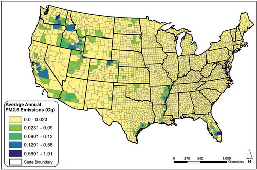
The county-level distribution of CO and PM_2.5 emissions from crop residue burning reveal that within source states, much of the crop residue burning is clustered in a few counties (e.g., Florida, Texas) and/or a small subregion (e.g., Arkansas, Washington, California) (Figures 1 and 2). Additionally, although there is a strong spatial similarity between the CO and PM_2.5 county-level emissions, there were more than 30 fewer counties with above-average PM_2.5 emissions. This difference occurred mainly in wheat-producing regions in the Great Plains, the Rocky Mountain West, and the Pacific Northwest.

Figure 1. Average annual CO emissions (Gg) from crop residue burning by county for the CONUS (projection: Albers Equal Area Conic).

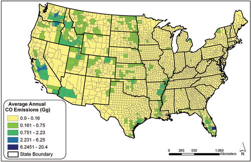
Figure 2. Average annual PM_2.5 emissions (Gg) from crop residue burning by county for the CONUS (projection: Albers Equal Area Conic).

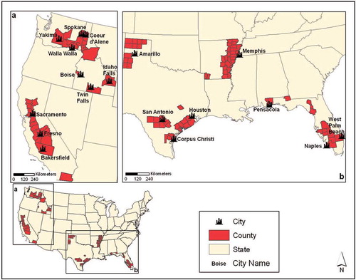
The total population in the counties and cities contained within and/or contiguous to crop residue burning areas was approximately 15.5 million people according to the 2007 and 2008 population estimates from the U.S. Census Bureau56,57 (Figure 3). This population, potentially affected by crop residue burning, is approximately 5.2% of the total population of the CONUS. Within the states, the proportion of people living within these source areas is higher; for example, 13.8% of the total population in Texas lives in counties, with the highest emissions being from crop residue burning. In Washington, 17.5% of the state's population resides in the source counties, which is similar to California (17.3%) and Florida (17.9%). Approximately 25% of the population in Arkansas lives in the source counties and almost half of the population of Idaho (46.6%) resides in the counties with the highest emissions from crop residue burning. At the very least, 1 in 10 people in the states of Arkansas, California, Florida, Idaho, Texas, and Washington live near the consistent source of emissions from crop residue burning.

Figure 3. Source counties of crop residue burning emissions. Cities contained within and/or contiguous to these source counties are labeled (projection: Albers Equal Area Conic).

Monthly and Seasonal Variability of Regional Emissions

A regional analysis of calculated emissions was completed in which regions were defined as the EPA regions. Five EPA regions (4, 6, 10, 8, and 7) were determined to be the main sources of emissions from crop residue burning (Figure 4). These five source regions represent approximately 82% of CO₂, 94% of CH₄, 91% of CO, 86% of NO₂ and SO₂, and 95% of PM_2.5 and PM₁₀ emissions for the CONUS.

Figure 4. EPA source regions of crop residue burning emissions (projection: Albers Equal Area Conic).

The monthly distribution of average CO emissions from crop residue burning for five EPA source regions showed that nearly every region experienced peaks of CO emissions between the months of April to July and September to November, corresponding to the spring harvest and fall harvest that occurs throughout much of the CONUS (Figure 5). Region 4 was an exception. Although there was a small spring peak between April and June and an increase of burning beginning in September, the largest peaks of CO emissions for region 4 spanned from November to February. The multiyear harvest was directly related to the sugarcane harvesting in Florida, which occurs between October and March.58 Region 6, with sugarcane growing areas in Louisiana and Texas, showed a smaller decrease in emissions in November and December compared with the other regions but retained higher emissions levels.

Figure 5. Monthly distribution of average CO emissions from crop residue burning by EPA source region for years 2003–2007.

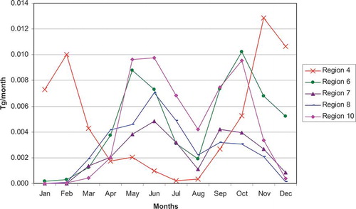
Emissions from these five major source regions showed considerable seasonal variability. This analysis defined seasons as winter (January to March); spring (April to June), summer (July to September), and fall (October to December). In general, the highest average monthly emissions of CO for the EPA source regions occurred in the spring and fall. Region 8, dominated by summer wheat harvesting in the northern Great Plains, had a continual increase in emissions from winter to spring, leveled off in summer related to the continuing wheat harvest, and a decrease in the fall. Similarly, region 6 has spring and summer wheat harvesting in the southern Great Plains, but it showed a sharp increase in emissions in the fall because of sugarcane and rice harvesting in the Mississippi Delta and Texas. Regions 7 and 10 had similar trends with a peak in summer burning and nearly equal amounts of burning in the spring and fall. Both of these regions are home to major wheat production, with the most burning in region 7 during the summer and the most wheat residue burning in region 10 during the spring, summer, and fall because of a double wheat crop system. Higher summer burning (in July and August) in region 10 is also due to Kentucky bluegrass seed harvesting (Figure 5). The seasonality of CO emissions for region 4 is nearly the opposite of the other regions, with the lowest amount of burning in spring and summer, and the most burning in winter and fall, particularly November through February, because of sugarcane in Florida and the fall harvest of rice and soy in other southeastern states.

Between the years 2003 and 2007, 34% of all emissions originated from sugarcane residue burning (Figure 6). Wheat residue burning accounted for 22% of all emissions, followed by rice with 14% of total emissions. Other crops/ fallow, Kentucky bluegrass seed, soybean, cotton, corn, and lentils accounted for 10% or less of all emissions, respectively. The results do not match the EPA estimate of crop residue burning by crop type. EPA estimates that 77% of all crop residue burning emissions are released from corn and soybean residue burning, with only 23% of emissions attributed to sugarcane (3%), wheat (10%), and rice (10%).42

Figure 6. Average contribution of emissions by crop type for the EPA source regions for years 2003–2007.

Interannual Variability of Crop Residue Burning Emissions for the CONUS

On average, annual crop residue burning in the CONUS emitted 6.1 Tg of CO₂, 8.9 Gg of CH₄, and 232.4 Gg of CO per year (Table 5). PM₁₀ and PM_2.5 emissions were an average of 28.5 and 20.9 Gg, respectively. NO₂ and SO₂ were less, with average emissions of 10.6 and 4.4 Gg, respectively. Emissions from CO, PM_2.5, and PM₁₀ were the most significant in terms of quantity.

Table 5. Total and average carbon and air quality emissions from crop residue burning for the CONUS, 2003–2007, including interannual variability

Years	CO2	CH4	CO	NO2	SO2	PM2.5	PM10
2003	6.46	9.03	247	11.6	4.95	21.9	29.4
2004	6.03	8.95	234	10.7	4.41	21.3	28.1
2005	6.07	9.14	234	10.6	4.29	21.4	29.1
2006	5.72	8.19	208	9.22	3.60	18.8	26.4
2007	6.15	9.07	239	11.0	4.59	21.4	29.3
Total	30.5	44.4	1160	53.0	21.8	105	142
Average	6.09	8.87	232	10.6	4.37	20.9	28.5
Average interannual variability (± value)	0.31	0.52	18.0	1.03	0.59	1.51	1.95
Average interannual variability (%)	5.07	5.90	7.76	9.70	13.5	7.20	7.03
Notes: CO2 reported in Tg yr^−1; all other species reported in Gg yr^−1. All numbers are rounded to three significant figures.

The average interannual variability was higher for the emissions of CO, NO₂, SO₂, PM_2.5, and PM₁₀ than the carbon emissions of CO₂ and CH₄ (Table 5). The highest average interannual variability was calculated for SO₂ at 13.4%, followed by NO₂ at 9.7%. Particulate emissions from crop residue burning, PM_2.5 and PM₁₀, had an average interannual variability of 7.2%, slightly below the CO average interannual variability of 7.8%. In general, in addition to SO₂, air quality and carbon emissions from crop residue burning in the CONUS varied less than 10% interannually.

COMPARISON WITH PUBLISHED EMISSION ESTIMATES

Comparison with Agricultural Emissions

The results of this analysis were compared with global estimates of crop residue burning17,34 and North American estimates of agricultural burning.18 Two of these studies, Andreae and Merlet34 and Wiedinmyer et al.,18 grouped all agricultural emissions and did not specify by crop type. Yevich and Logan17 did specify by crop type, although that study and this analysis did not completely share the same crop types; that is, Kentucky bluegrass seed. The CONUS crop residue burning accounted for an average of 1% of total global CO₂, CO, CH₄, PM_2.5, and SO₂ emissions from crop residue burning calculated by Andreae and Merlet34(Table 6). Comparing the three atmospheric species of CO₂, CO, and CH₄, calculated by Andreae and Merlet34 and Yevich and Logan,17 the average CONUS emissions for the same species (i.e., an averaging of the comparison percentages for CO₂, CO, and CH₄) accounted for 0.6 and 2.1% of total global emissions from these two sources, respectively. The North American estimates from Wiedinmyer et al.18 included all forms of agricultural burning in much of Central America, Mexico, the United States, and Canada. Estimates from this study accounted for an average of 15.1% of total CO and PM_2.5 emissions from agricultural burning in North America.18 Although crop residue burning in the CONUS was a minor source of agricultural burning emissions on a global scale, it appeared to be a significant source within North America.

Table 6. Comparison of global, continental, and U.S. agricultural, forest, and total burning emissions with estimated emissions from this analysis

Source	Scale (Land Cover)	CO2	CO	CH4	PM2.5	SO2
Andreae and Merlet34	Global (agricultural)	818	50.0	1.50	2.10	0.22
Yevich and Logan17	Global (agricultural)	140	23.0	1.00	—	—
Wiedinmyer et al.18	North America (agricultural)	—	1.62	—	0.13	—
Wiedinmyer et al.18	North America (forest)	—	44.2	—	5.10	—
Wiedinmyer et al.18	United States (total pyrogenic)	356	19.8	1.00	2.40	0.16
This analysis	CONUS	6.09	0.23	8.88 × 10^−3	2.09 × 10^−2	4.37 × 10^−3
Andreae and Merlet34	Percent CONUS cropland fire emissions	0.74	0.46	0.59	1.00	1.98
Yevich and Logan17	Percent CONUS cropland fire emissions	4.35	1.01	0.89	—	—
Wiedinmyer et al.18: North America (agricultural)	Percent CONUS cropland fire emissions	—	14.3	—	15.9	—
Wiedinmyer et al.18: North America (forest)	Percent CONUS cropland fires emissions	—	0.53	—	0.41	—
Wiedinmyer et al.18: United States (total pyrogenic)	Percent CONUS cropland fires emissions	1.71	1.17	0.89	0.87	2.73
Notes: The percent CONUS cropland fire emission values were calculated by dividing the average CONUS crop residue burning emissions by the published estimates of agricultural, forest, and total burning emissions. Emissions are reported in Tg yr^−1. All numbers are rounded to three significant figures.

Comparison with Wildfire Emissions

Wildfire emissions are an important source of carbon and air quality emissions at the global, continental, and regional scale.34,40,59,60 CONUS crop residue burning emissions were compared with North American estimates of forest fires and total pyrogenic emissions from all burning sources for the United States, including Alaska and Hawaii.18 CONUS crop residue burning emissions accounted for approximately 0.5% of total emissions of CO and PM_2.5 from forest fires in North America (Table 6). However, crop residue burning did account for a higher average of emissions in the United States, averaging 1.5% of total CO₂, CO, CH₄, PM_2.5, and SO₂ emissions from all fires.

Implications for the EPA National Emissions Inventory

The EPA National Emissions Inventory (NEI) currently includes pyrogenic sources of air pollution. In 2002, the NEI did provide explicit emission estimates from fires, grouped together in one class that included agricultural fires, prescribed/slash burning, wildfires, structural fires, and other burning.61 The 2002 NEI burning estimates for agricultural fires were limited to 23 states and included burning activity ranging from pasture maintenance fires, burn piles, and crop residue burning.19 Subsequent NEI reports for 2005 and 2008 have relied on the agricultural fire emissions estimated from 2002. The average emissions from this analysis were compared with the 2002 NEI fire emissions. The average annual crop residue burning emissions from this analysis accounted for approximately 1.4% of total CO, 1.5% of total PM_2.5, 1.7% of total PM₁₀, and 0.3% of total SO₂ emissions of all burning activity reported in the 2002 NEI. Future NEI reports would benefit from separating different categories of fire activities to determine the relative contributions of the different burning sources and whether agricultural burning (i.e., crop residue fire emissions) is a significant contributor to total pyrogenic emissions.

Implications for the EPA Greenhouse Gas Emissions Inventory

EPA annually prepares an inventory of national greenhouse gas sources and sinks for the United States. The most recent publication, the 2008 Inventory of Greenhouse Gas Emissions and Sinks,42 included CH₄ and CO emissions estimates from field burning of agricultural residues for the years 1990–2006. Crops included in the EPA Greenhouse Gas Inventory included barley, corn, peanuts, rice, soybean, sugarcane, and wheat. This analysis did not include barley and peanuts; however, emissions from these two crops accounted for less than 3% of the total emissions reported by the EPA. Methodologies for emission estimates were different, with the largest divergence coming from the emission factors, the fraction of residue burned (CE), fuel load, and the burned area estimates. The greatest uncertainty in the EPA emissions calculations was fuel load (discussed below), noted in the Greenhouse Gas Inventory document.42 In the case of the emission factors, the EPA greenhouse inventory used their own emission factors from the EPA AP-42 document43 and this analysis used calculated emission factors from the scientific literature that included the EPA emission factors, as reported by Dennis et al.11 The CE factor used by the EPA was 0.88, 15% higher than the average CE factor used by this analysis of 0.75. As for burned area, the EPA assumed that 3% of the area for all targeted crops burned, except for rice.42 Burned rice acreages were taken from state estimates. Combining these estimates, the EPA assumed a cropland burned area that was on average 2 times the area that was detected by the hybrid remote sensing approach used in this analysis.9

Fuel loads have been noted as having high uncertainty values in bottom-up emissions calculations.62 As previously mentioned, the EPA methodology for fuel load calculation outlined in the Greenhouse Gas Inventory42 was not utilized in this analysis. Four crops common to this analysis and the 2008 EPA Greenhouse Gas Inventory were corn, rice, sugarcane, and wheat. The EPA Greenhouse Gas Inventory estimated emissions using higher fuel load variables for the crops of rice (33% higher) and sugarcane (71%). The fuel load values from this analysis and the Greenhouse Gas Inventory were the same for wheat: Both studies utilized an estimate of 2752 kg/ha. Corn was the exception, with this analysis utilizing a fuel load estimate that was 38% higher than the EPA's fuel load variable.

Table 7 shows the comparison of the 2008 EPA estimates with this analysis, including the crop residue burning emissions calculated using the average emissions factors and the maximum emission factors. This analysis estimated CH₄ and CO emissions to be an average of 78 and 73% less than the EPA estimates, respectively. Using the maximum emission factors, the average annual emissions from crop residue burning for CH₄ and CO were 0.017 and 0.972 Tg, respectively. These maximum CH₄ and CO emissions were 52 and 23% higher than the emissions calculated from the average emission factors, respectively. The CH₄ and CO emission estimates calculated using the maximum emission factor values accounted for 50 and 119%, respectively, of the average annual EPA estimation of CH₄ and CO emissions from crop residue burning. On the basis of the results of this analysis, it is likely that the EPA is overestimating CH₄ emissions from crop residue burning. However, the CO emissions reported by the EPA fall within the range of emission estimates from this analysis calculated using the average and maximum emission factors. Therefore, the EPA estimation of CO emissions of crop residue burning appears reasonable.

Table 7. Comparison of CH₄ and CO emissions from crop residue burning estimated by the 2008 EPA Greenhouse Gas Inventory with results from this analysis for 2003–2006

	Species	2003	2004	2005	2006	Average
EPA	CH4	0.04	0.04	0.04	0.04	0.04
	CO	0.80	0.88	0.86	0.83	0.84
This analysis (average emission factors)	CH4	9.00 × 10^−3	9.00 × 10^−3	9.00 × 10^−3	8.00 × 10^−3	9.00 × 10^−3
	CO	0.25	0.23	0.23	0.21	0.23
This analysis (maximum emission factors)	CH4	0.02	0.02	0.02	0.02	0.02
	CO	1.05	1.00	1.00	0.96	1.00
Percent CONUS cropland burning emissions in the EPA estimates from average emissions (%)	CH4	22.5	22.5	22.5	20.0	21.9
	CO	31.3	26.1	26.7	25.3	27.4
Percent CONUS cropland burning emissions in the EPA estimates from maximum emissions (%)	CH4	50.0	50.0	50.0	50.0	50.0
	CO	131	114	116	116	119
Notes: Emissions from this analysis calculated using the average emission factors and the maximum emission factors. Emissions are reported in Tg yr^−1. All numbers are rounded to three significant figures.

Crop residue burning emissions are a minor source of CH₄ emissions compared with the CH₄ emissions from other agricultural sources. Crop residue burning emissions accounted for less than 1% of the annual emissions from enteric fermentation, manure management, and rice cultivation reported in the EPA Greenhouse Gas Inventory.42 Specifically, crop residue burning in the CONUS accounted for an average 0.11% of annual CH₄ emissions from enteric fermentation, 0.15% of manure managements, and 0.45% of rice cultivation.

The USDA also compiles a Greenhouse Gas Inventory focused on CH₄ and CO emissions from agricultural and forestry sources using the crop residue burning emission estimates from the EPA Greenhouse Gas Inventory.63 The USDA ranks the states of Iowa, Illinois, Minnesota, Nebraska, Arizona, Indiana, Kansas, Arkansas, Ohio, and South Dakota (in descending order) as the largest sources of CH₄ emissions. In general, this analysis showed that a different set of states are the main sources of CH₄ emissions from crop residue burning (in descending order): Idaho, Washington, Florida, Texas, Arkansas, Kansas, Oregon, South Dakota, North Dakota, and Missouri. The states of Arkansas, Kansas, and South Dakota were shared between the two studies. The USDA Greenhouse Gas Inventory overestimates the contribution of crop residue burning emissions from the midwestern states of Illinois, Iowa, Indiana, Minnesota, Nebraska, and Ohio.

CONCLUSIONS

Most crop residue burning emissions in the CONUS were emitted in the spring, summer, and fall. CONUS crop residue burning emissions had an average interannual variability of ±10%, ranging from 5.1% for CO₂ and 13.4% for SO₂. Six states emitted the most air quality and carbon emissions from crop residue burning (ranked in descending order): Florida, Washington, Texas, California, Idaho, and Arkansas. These six states accounted for 50% of PM₁₀, 51% of CO₂, 52% of CO, and 63% of PM_2.5. Florida alone emitted 17% of all annual CO₂, CO, and PM_2.5 emissions as well as 12% of all annual PM₁₀ emissions from crop residue burning. From a regional perspective, EPA regions 4, 6, 10, 8, and 7 (in descending order) were the main sources of emissions. These five EPA regions, comprising the southeastern United States, the Great Plains, and the Pacific Northwest, represented 85% of all emission for crop residue burning for the atmospheric species of CO₂, CO, CH₄, NO₂, SO₂, PM_2.5, and PM₁₀. Approximately 70% of all crop residue burning emissions in the EPA source regions originated from the three crops of sugarcane, wheat, and rice.

Compared with estimates of all agricultural burning emissions in North America, which included all types of agricultural burning, which included slash-and-burn, land clearing, pasture maintenance, etc., the CONUS crop residue burning emissions represented 15% of total emissions. CONUS crop residue burning emissions were also significantly less than estimated wildfire emissions. Forest fire emissions in North America of CO and PM_2.5 were significantly higher than the estimates from this analysis, with cropland burning being approximately equivalent to 0.5% of North American forest fire emissions. At the national level, crop residue burning emission estimates accounted for 1.5% of total CO₂, CO, CH₄, PM_2.5, and SO₂ emissions from all pyrogenic emissions in the United States, including Alaska and Hawaii. Results from this analysis show that crop residue burning emission estimates accounted for 6% of total emissions from current fire emission estimates reported by the EPA NEI.

This analysis provided an independent assessment of crop residue burning not dependent on the self-reporting of state agencies. Future EPA reports could incorporate this work to better account for crop residue burning. Compared with this study, the EPA reports, which have relied on self-reporting, consistently overestimated cropland burned area by a factor of 2 and overestimated crop residue burning CH₄ emissions in the Midwest instead of the southeastern United States and Pacific Northwest. The EPA estimates of CO and CH₄ were 73–78% higher than the CO and CH₄ emission estimates from this analysis, respectively. However, when emissions are calculated using the maximum emission factor values, the EPA estimates of CH₄ were 50% higher than this analysis whereas the EPA estimates of CO were 19% lower than this analysis. On the basis of these results, it is likely that the EPA is overestimating CH₄ emissions but current CO emissions are well within the ranges estimated by this analysis. This analysis also showed that crop residue burning emissions are a minor source of CH₄ emissions (<1%) compared with the CH₄ emissions from other agricultural sources, specifically enteric fermentation, manure management, and rice cultivation.

REFERENCES

- Korontzi , S. , McCarty , J. , Loboda , T. , Kumar , S. and Justice , C.O. 2006 . Global Distribution of Agricultural Fires from Three Years of MODIS Data . Global Biogeochem. Cy. , 20 : 2021 doi: 10.1029/2005GB002529
- McCarty , J.L. , Justice , C.O. and Korontzi , S. 2007 . Agricultural Burning in the Southeastern United States Detected by MODIS . Remote Sens. Environ. , 108 : 151 – 162 . doi: 10.1016/j.rse.2006.03.020
- Witham , C. and Manning , A. 2007 . Impacts of Russian Biomass Burning on UK Air Quality . Atmos. Environ. , 41 : 8075 – 8090 . doi: 10.1016/j.atmosenv.2007.06.058
- Yang , S.J. , He , H.P. , Lu , S.L. , Chen , D. and Zhu , J.X. 2008 . Quantification of Crop Residue Burning in the Field and Its Influence on Ambient Air Quality in Suqian, China . Atmos. Environ. , 42 : 1961 – 1969 . doi: 10.1016/j.atmosenv.2007.12.007
- Chen , K.S. , Wang , H.K. , Peng , Y.P. , Wang , W.C. , Chen , C.H. and Lai , C.H. 2008 . Effects of Open Burning of Rice Straw on Concentration of Atmospheric Polycyclic Aromatic Hydrocarbons in Central Taiwan . Journal of the Air & Waste Management Association , 58 : 1318 – 1327 . doi: 10.3155-1047-3289.58.10.1318
- Wulfhorst , J.D. , Van Tassell , L. , Johnson , B. , Holman , J. and Thill , D. 2006 . An Industry Amidst Conflict and Change: Practices and Perceptions of Idaho's Bluegrass Seed Producers , Moscow , ID : University of Idaho College of Agricultural and Life Sciences . RES-165
- Canode , C.L. and Law , A.G. 1979 . Thatch and Tiller Size as Influenced by Residue Management in Kentucky Bluegrass Seed Management . Agron J. , 71 : 289 – 291 .
- Dhammapala , R. , Claiborn , C. , Corkill , J. and Gullett , B. 2006 . Particulate Emissions from Wheat and Kentucky Bluegrass Stubble Burning in Eastern Washington and Northern Idaho . Atmos. Environ. , 40 : 1007 – 1015 . doi: 10.1016/j.atmosenv.2005.11.018
- McCarty , J.L. , Korontzi , S. , Justice , C.O. and Loboda , T. 2009 . The Spatial and Temporal Distribution of Crop Residue Burning in the Contiguous United States . Sci. Total Environ. , 407 : 5701 – 5712 . doi: 10.1016/j.scitotenv.2009.07.009
- Jenkins , B.M. , Turn , S.Q. and Williams , R.B. 1992 . Atmospheric Emissions from Agricultural Burning in California: Determination of Burn Fractions, Distribution Factors, and Crop-Specific Contributions . Agr. Ecosyst. Environ. , 38 : 313 – 330 . doi: 10.1016/0167-8809(92)90153-3
- Dennis , A. , Fraser , M. , Anderson , S. and Allen , D. 2002 . Air Pollutant Emissions Associated with Forest, Grassland, and Agricultural Burning in Texas . Atmos. Environ. , 36 : 3779 – 3792 . doi: 10.1016/S1352-2310(02)00219-4
- Jimenez , J.R. , Claiborn , C.S. , Dhammapala , R.S. and Simpson , C.D. 2007 . Methoxyphenols and Levoglucosan Ratios in PM2.5 from Wheat and Kentucky Bluegrass Stubble Burning in Eastern Washington and Northern Idaho . Environ. Sci. Technol. , 41 : 7824 – 7829 .
- Ezcurra , A.T. , de Zárate , I.O. , Lacaux , J.-P. and Dinh , P.-V . 1996 . Biomass Burning and Global Change , Edited by: Levine , J.S . 73 – 78 . Cambridge , MA : Massachusetts Institute of Technology .
- Zhang , Y. , Cao , M. , Wang , X. and Yao , H. 1996 . Biomass Burning and Global Change; Levine, J.S , 764 – 770 . Cambridge , MA : Massachusetts Institute of Technology .
- Andreae , M.O. 1991 . Global Biomass Burning: Atmospheric, Climatic, and Biosphere Implications , Edited by: Levine , J.S . 3 – 21 . Cambridge , MA : Massachusetts Institute of Technology .
- Hao , W.M. and Liu , M.-H. 1994 . Spatial and Temporal Distribution of Tropical Bio-mass . Global Biogeochem. Cy. , 21 : 495 – 503 . doi: 10.1029/94GB02086
- Yevich , R. and Logan , J.A. 2003 . An Assessment of Biofuel Use and Burning of Agricultural Waste in the Developing World . Global Biogeochem. Cy. , 17 : 1095 doi: 10.1029/2002GB001952
- Wiedinmyer , C. , Quayle , B. , Geron , C. , Belote , A. , McKenzie , D. , Zhang , X. , O'Neill , S. and Wynne , K.K. 2006 . Estimating Emissions from Fires in North America for Air Quality Modeling . Atmos. Environ. , 40 : 3419 – 3432 . doi: 10.1016/j.atmosenv.2006.02.010
- Pouliot , G. , Pace , T. , Roy , B. , Pierce , T. and Mobley , D. 2008 . Development of a Biomass Burning Emissions Inventory by Combining Satellite and Ground-Based Information . J. Appl. Remote Sens. , 2 : 021501 doi: 10.1117/1.2939551
- Al-Saadi , J. , Soja , A. , Pierce , R.B. , Szykman , J. , Wiedinmyer , C. , Emmons , L. , Kondragunta , S. , Zhang , X. , Kittaka , C. , Schaack , T. and Bowman , K. 2008 . Intercomparison of Near-Real-Time Biomass Burning Emissions Estimates Constrained by Satellite Fire Data . J. Appl. Remote Sens. , 2 : 021504 doi: 10.1117/1.2948785
- North American Carbon Program http://www.esig.ucar.edu/nacp/nacp.pdf (http://www.esig.ucar.edu/nacp/nacp.pdf) (Accessed: 2010 ).
- National Ambient Air Quality Standards (NAAQS); U.S. Environmental Protection Agency http://epa.gov/air/criteria.html (http://epa.gov/air/criteria.html) (Accessed: 2010 ).
- Korontzi , S. , McCarty , J. and Justice , C. 2008 . Monitoring Agricultural Burning in the Mississippi River Valley Region from the Moderate Resolution Imaging Spectroradiometer (MODIS) . Journal of the Air & Waste Management Association , 58 : 1235 – 1239 . doi: 10.3155-1047-3289.58.9.1235
- McCarty , J.L. , Loboda , T. and Trigg , S. 2008 . A Hybrid Remote Sensing Approach to Quantifying Crop Residue Burning in the United States . Appl. Eng. Agric. , 24 : 515 – 527 .
- Vermote , E.F. , El Saleous , N.Z. and Justice , C.O. 2002 . Atmospheric Correction of MODIS Data in the Visible to Middle Infrared: First Results . Remote Sens. Environ. , 83 : 97 – 111 . doi: 10.1016/S0034-4257(02)00089-5
- Giglio , L. , Descloitres , J. , Justice , C.O. and Kaufman , Y.J. 2003 . An Enhanced Contextual Fire Detection Algorithm for MODIS . Remote Sens. Environ. , 87 : 273 – 282 . doi: 10.1016/S0034-4257(03)00184-6
- Hansen , M.C. , DeFries , R.S. , Townshend , J.R.G. , Marufu , L. and Sohlberg , R . 2002 . Development of a MODIS Tree Cover Validation Data Set for Western Province, Zambia . Remote Sens. Environ. , 83 : 320 – 335 . doi: 10.1016/S0034-4257(02)00080-9
- Wardlow , B.D. , Kastens , J.H. and Egbert , S.L. 2006 . Using USDA Crop Progress Data and MODIS Time-Series NDVI for Regional-Scale Evaluation of Greenup Onset Date . Photogramm. Eng. Rem. S. , 72 : 1225 – 1234 .
- Chang , J. , Hansen , M.C. , Pittman , K. , Carroll , M. and Dimiceli , C. 2007 . Corn and Soybean Mapping in the United States Using MODIS Time-Series Data Sets . Agron. J. , 99 : 1654 – 1664 . doi: 10.2134/agronj2007.0170
- A History of the Cropland Data Layer at NASS; U.S. Department of Agriculture National Agricultural Statistics Service http://www.nass.usda.gov/research/Cropland/CDL_History_MEC.pdf (http://www.nass.usda.gov/research/Cropland/CDL_History_MEC.pdf) (Accessed: 2010 ).
- IPCC Emission Factors Database; Intergovernmental Panel on Climate Change http://www.ipcc-nggip.iges.or.jp/EFDB/main.php (http://www.ipcc-nggip.iges.or.jp/EFDB/main.php) (Accessed: 2006 ).
- Jenkins , B.M. , Turn , S.Q. and Williams , R.B. 1996 . Atmospheric Pollutant Emission Factors from Open Burning of Agricultural and Forest Biomass by Wind Tunnel Simulations , Vol. 2 , Sacramento , CA : California Air Resources Board . Project No. A932-126
- United Kingdom Emission Factor Database; U.K. National Atmospheric Emissions Inventory http://www.naei.org.uk/emissions/selection.php (http://www.naei.org.uk/emissions/selection.php) (Accessed: 2006 ).
- Andreae , M.O. and Merlet , P. 2001 . Emission of Trace Gases and Aerosols from Biomass Burning . Global Biogeochem. Cy. , 15 : 955 – 966 . doi: 10.1029/2000GB001382
- Cereal-Grain Residue Open-Field Burning Emissions Study; Air Sciences http://www.ecy.wa.gov/programs/air/aginfo/research_pdf_files/FinalWheat_081303.pdf (http://www.ecy.wa.gov/programs/air/aginfo/research_pdf_files/FinalWheat_081303.pdf) (Accessed: 2006 ).
- Quantifying Post-Harvest Emissions from Bluegrass Seed Production Field Burning; Washington State Department of Ecology, Air Quality, Ag Burning Research http://www.ecy.wa.gov/programs/air/aginfo/research_pdf_files/FinalKBGEmissionStudyReport_4504.pdf (http://www.ecy.wa.gov/programs/air/aginfo/research_pdf_files/FinalKBGEmissionStudyReport_4504.pdf) (Accessed: 2006 ).
- Lemieux , P.M. , Lutes , C.C. and Santoianni , D.A. 2004 . Emissions of Organic Air Toxics from Open Burning: A Comprehensive Review . Prog. Energ. Combus. , 30 : 1 – 32 . doi: 10.1016/j.pecs.2003.08.001
- Hays , M.D. , Fine , P.M. , Geron , C.D. , Kleemand , M.J. and Gullett , B.K. 2005 . Open Burning of Agricultural Biomass: Physical and Chemical Properties of Particle-Phase Emissions . Atmos. Environ. , 39 : 6747 – 6764 . doi: 10.1016/j.atmosenv.2005.07.072
- Integrated Assessment Update and 2018 Emissions Inventory for Prescribed Fire, Wildfire, and Agricultural Burning; Western Regional Air Partnership http://www.wrapair.org/forums/fejf/documents/emissions/WGA2018report20051123.pdf (http://www.wrapair.org/forums/fejf/documents/emissions/WGA2018report20051123.pdf) (Accessed: 2008 ).
- Seiler , W. and Crutzen , P.J. 1980 . Estimates of Gross and Net Fluxes of Carbon between the Biosphere and the Atmosphere from Biomass Burning . Climatic Change , 2 : 207 – 247 . doi: 10.1007/BF00137988
- Kasischke , E.S. and Penner , J.E. 2004 . Improving Global Estimates of Atmospheric Emissions from Biomass Burning . J. Geophys. Res. , 109 : 1 – 9 . doi: 10.1029/2004JD004972
- Inventory of U.S. Greenhouse Gas Emissions and Sinks: 1990–2006; U.S. Environmental Protection Agency http://www.epa.gov/climatechange/emissions/downloads/08_CR.pdf (http://www.epa.gov/climatechange/emissions/downloads/08_CR.pdf) (Accessed: 2008 ).
- 1994 . International Anthropogenic Methane Emissions: Estimates for 1990 , Washington , DC : U.S. Environmental Protection Agency . EPA 230-R-93-010
- 1992 . Compilation of Air Pollution Emission Factors, Volume I: Stationary Point and Area Sources , 5th , Research Triangle Park , NC : U.S. Environmental Protection Agency . AP-42 (GPO 055-000-00500-1)
- 2003 Acreage; Agricultural Statistics Board, National Agricultural Statistics Service, U.S. Department of Agriculture http://usda.mannlib.cornell.edu/usda/nass/Acre//2000s/2003/Acre-06-30-2003.pdf (http://usda.mannlib.cornell.edu/usda/nass/Acre//2000s/2003/Acre-06-30-2003.pdf) (Accessed: 2007 ).
- 2004 Acreage; Agricultural Statistics Board, National Agricultural Statistics Service, U.S. Department of Agriculture http://usda.mannlib.cornell.edu/usda/nass/Acre//2000s/2004/Acre-06-30-2004.pdf (http://usda.mannlib.cornell.edu/usda/nass/Acre//2000s/2004/Acre-06-30-2004.pdf) (Accessed: 2007 ).
- 2005 Acreage; Agricultural Statistics Board, National Agricultural Statistics Service, U.S. Department of Agriculture http://usda.mannlib.cornell.edu/usda/nass/Acre//2000s/2005/Acre-06-30-2005.pdf (http://usda.mannlib.cornell.edu/usda/nass/Acre//2000s/2005/Acre-06-30-2005.pdf) (Accessed: 2007 ).
- 2006 Acreage; Agricultural Statistics Board, National Agricultural Statistics Service, U.S. Department of Agriculture http://usda.mannlib.cornell.edu/usda/nass/Acre//2000s/2006/Acre-06-30-2006.pdf (http://usda.mannlib.cornell.edu/usda/nass/Acre//2000s/2006/Acre-06-30-2006.pdf) (Accessed: 2007 ).
- 2007 Acreage; Agricultural Statistics Board, National Agricultural Statistics Service, U.S. Department of Agriculture http://usda.mannlib.cornell.edu/reports/nassr/field/pcp-bba/acrg0607.pdf (http://usda.mannlib.cornell.edu/reports/nassr/field/pcp-bba/acrg0607.pdf) (Accessed: 2007 ).
- Strehler , A. and Stutzle , G. 1987 . Biomass: Regenerable Energy , Edited by: Hall , D.O. and Over-end , R.P. 75 – 102 . London , , United Kingdom : Elsevier .
- Cramer , G. 2008 . Kansas State University, Wichita, KS. Personal communication
- Turn , S.Q. , Jenkins , B.M. , Chow , J.C. , Pritchett , L.C. , Campbell , D. , Cahill , T. and Whalen , S.A. 1997 . Elemental Characterization of Particulate Matter Emitted from Biomass Burning: Wind Tunnel Derived Source Profiles for Herbaceous and Wood Fuels . J. Geophys. Res. , 102 : 3863 – 3699 . doi: 10.1029/96JD02979
- EPA Air Quality Systems Database; U.S. Environmental Protection Agency http://www.epa.gov/oar/data/aqsdb.html (http://www.epa.gov/oar/data/aqsdb.html) (Accessed: 2010 ).
- Hoff , R. , Zhang , H. , Jordan , N. , Prados , A. , Engel-Cox , J. , Huff , A. , Weber , S. , Zell , E. , Kondragunta , S. , Szykman , J. , Johns , B. , Dimmick , F. , Wimmers , A. , Al-Saadi , J. and Kittaka , C. 2009 . Applications of the Three-Dimensional Air Quality System to Western U.S. Air Quality: IDEA, Smog Blog, Smog Stories, AirQuest, and the Remote Sensing Information Gateway . Journal of the Air & Waste Management Association , 59 : 980 – 989 . doi: 10.3155-1047-3289.59.8.980
- Kühlwein , J. and Friedrich , R. 2000 . Uncertainties of Modeling Emissions from Road Transport . Atmos. Environ. , 34 : 4603 – 4610 . doi: 10.1016/S1352-2310(00)00302-2
- 2007 Population Estimate; U.S. Census Bureau https://factfinder.census.gov (https://factfinder.census.gov) (Accessed: 2009 ).
- 2008 Population Estimate; U.S. Census Bureau https://factfinder.census.gov (https://factfinder.census.gov) (Accessed: 2009 ).
- Florida Sugarcane Handbook; University of Florida, Institute of Food and Agricultural Science, Florida Cooperative Extension Service: Gainesville, FL http://edis.ifas.ufl.edu/pdffiles/SC/SC03200.pdf (http://edis.ifas.ufl.edu/pdffiles/SC/SC03200.pdf) (Accessed: 2008 ).
- Liu , Y. 2004 . Variability of Wildland Fire Emissions across the Contiguous United States . Atmos. Environ. , 38 : 3489 – 3499 . doi: 10.1016/j.atmosenv.2004.02.004
- Yokelson , R.J. , Christian , T.J. , Karl , T.G. and Guenther , A. 2008 . The Tropical Forest and Fire Emissions Experiment: Laboratory Fire Measurements and Synthesis of Campaign Data . Atmos. Chem. Phys. , 8 : 3509 – 3527 . doi: 10.5194/acp-8-3509-2008
- 2002 National Emissions Inventory Booklet; U.S. Environmental Protection Agency http://www.epa.gov/ttn/chief/net/2002neibooklet.pdf (http://www.epa.gov/ttn/chief/net/2002neibooklet.pdf) (Accessed: 2008 ).
- Korontzi , S. , Roy , D.P. , Justice , C.O. and Ward , D.E. 2004 . Modeling and Sensitivity Analysis of Fire Emissions in Southern Africa during SAFARI 2000 . Remote Sens. Environ. , 92 : 255 – 275 . doi: 10.1016/j.rse.2004.06.010
- U.S. Agriculture and Forestry Greenhouse Gas Inventory: 1990–2005; U.S. Department of Agriculture Global Change Program Office http://www.usda.gov/oce/global_change/AFGGInventory1990_2005.htm (http://www.usda.gov/oce/global_change/AFGGInventory1990_2005.htm) (Accessed: 2008 ).