Impact of Biogenic Emission Uncertainties on the Simulated Response of Ozone and Fine Particulate Matter to Anthropogenic Emission Reductions

ABSTRACT

The role of emissions of volatile organic compounds and nitric oxide from biogenic sources is becoming increasingly important in regulatory air quality modeling as levels of anthropogenic emissions continue to decrease and stricter health-based air quality standards are being adopted. However, considerable uncertainties still exist in the current estimation methodologies for biogenic emissions. The impact of these uncertainties on ozone and fine particulate matter (PM_2.5) levels for the eastern United States was studied, focusing on biogenic emissions estimates from two commonly used biogenic emission models, the Model of Emissions of Gases and Aerosols from Nature (MEGAN) and the Biogenic Emissions Inventory System (BEIS). Photochemical grid modeling simulations were performed for two scenarios: one reflecting present day conditions and the other reflecting a hypothetical future year with reductions in emissions of anthropogenic oxides of nitrogen (NO_x). For ozone, the use of MEGAN emissions resulted in a higher ozone response to hypothetical anthropogenic NO_x emission reductions compared with BEIS. Applying the current U.S. Environmental Protection Agency guidance on regulatory air quality modeling in conjunction with typical maximum ozone concentrations, the differences in estimated future year ozone design values (DVF) stemming from differences in biogenic emissions estimates were on the order of 4 parts per billion (ppb), corresponding to approximately 5% of the daily maximum 8-hr ozone National Ambient Air Quality Standard (NAAQS) of 75 ppb. For PM_2.5, the differences were 0.1–0.25 μg/m³ in the summer total organic mass component of DVFs, corresponding to approximately 1–2% of the value of the annual PM_2.5 NAAQS of 15 μg/m³. Spatial variations in the ozone and PM_2.5 differences also reveal that the impacts of different biogenic emission estimates on ozone and PM_2.5 levels are dependent on ambient levels of anthropogenic emissions.

IMPLICATIONS

The findings presented in this study demonstrate that uncertainties in biogenic emission estimates due to different emission models can have a significant effect on the model estimates of ozone and PM_2.5 concentrations; specifically, the changes in these concentrations due to reductions in anthropogenic emissions considered in regulatory modeling scenarios. These results point to the need for further research aimed at improving biogenic emission estimates as well as better characterizing their dependency on environmental factors and the fate of these emissions once released into the atmosphere.

INTRODUCTION

The role of biogenic emissions in the secondary formation of ground-level air pollution has been the subject of numerous past modeling studies.1–8 For ozone, the primary biogenic compound of interest is isoprene because of itshigh reactivity.1 For fine particulate matter (PM_2.5), isoprene and mono- and sesquiterpenes are the species of greatest interest because they play a key role in the formation of secondary organic aerosols (SOAs) that comprise a substantial fraction of total PM_2.5, especially in the southeastern United States.9–14 On the basis of a regional modeling study, Tao et al.15 found that biogenic emissions contribute more than 40% to surface ozone concentrations in the northeastern United States, and that a large part of this contribution is due to the interactions between anthropogenic and biogenic emissions of volatile organic compounds (VOCs) and oxides of nitrogen (NO_x). As summarized by Fiore et al.,15 in current-generation chemical mechanisms these interactions depend on the relative magnitudes of NO_x and isoprene emissions. Nonlinear interactions between these emissions determine whether a given increase in isoprene emissions will enhance, deplete, or have little impact on surface ozone.3,7,8 In polluted areas, higher isoprene concentrations are generally understood to enhance ozone production because its oxidation increases the concentrations of hydroperoxy and organic peroxy radicals that can convert nitric oxide (NO) to nitrogen dioxide (NO₂) without destroying ozone. In areas with lower NO_x emissions, ozone production is typically limited by the availability of NO_x and shows little sensitivity to changes in isoprene. Finally, in chemical regimes characterized by very low NO_x and very high isoprene emissions, the reaction of ozone with isoprene becomes important, leading to a reduction of hydroxyl radicals (OH) and decreased ozone production. However, uncertainties in the chemical mechanism still exist, especially in relation to the isoprene oxidation chemistry used in current-generation chemical mechanisms.16–19

Because of the importance of biogenic emissions in atmospheric chemistry, improving their representation in chemical transport models continues to be an active area of research,1,5,20–22 with a focus on improving emission estimates and on better characterizing their fate once released into the atmosphere. However, at present, biogenic emission estimates used in global and regional air quality modeling applications continue to vary significantly, depending on the approach used. This is reflected in substantial revisions in emission estimates for subsequent releases of biogenic emission models5,23 and emission differences between different biogenic emission models.2,24 Additionally, several studies have highlighted major functional dependencies that are not considered in currently used biogenic emissions models, such as the effects of ambient carbon dioxide (CO₂) levels on plant production25 and plant damage due to ozone exposure.26 Likewise, the representation of the atmospheric fate of biogenic emissions in current-generation chemical mechanisms is still uncertain.16–19 In the context of future-year modeling over longer time horizons, additional uncertainties may arise because of insufficient consideration of potential climate change effects on the spatial distribution of different plant species and corresponding biogenic emissions.

Despite these continuing uncertainties, federal and state agencies rely on current-generation regional-scale air quality modeling tools to assess the impact of emission control strategies on ambient pollutant levels27–29 and to determine whether a geographic area attains an air quality standard in response to emissions reductions. In the United States, these current-generation tools include the Model of Emissions of Gases and Aerosols from Nature (MEGAN), version 2.04,20 and the Biogenic Emission Inventory System (BEIS), version 3.14,5,23,30,31 for estimating biogenic emissions and the Community Multiscale Air Quality (CMAQ) model32,33 and the Comprehensive Air Quality Model with Extensions34 for photochemical modeling. Although many modeling studies have investigated the effects of biogenic emission uncertainties on simulated ozone concentrations at regional and global scales,2,3,5–8,35,36 and on regional-scale SOA formation,37 most of these studies used a single anthropogenic emission base year inventory in their analyses. In contrast, in regional-scale air quality planning applications, a period of interest is simulated with at least two sets of anthropogenic emission inventories, one reflecting base year conditions and one or more additional inventories reflecting planned future year emissions.28 Few studies have explicitly considered the role of uncertainties in biogenic emissions on the effectiveness of emission control strategies in such regulatory applications. One notable exception is the study by Roselle,7 in which isoprene emissions were adjusted up or down by an uncertainty factor of 3 for base-case and control-case anthropogenic emission scenarios, and the impact on ozone levels was analyzed. The study results7 indicated that the response of calculated ozone levels to anthropogenic emission controls was sensitive to the magnitude of isoprene emissions. To the authors' knowledge, no comparable study has been performed to date to quantify the effect of biogenic emission uncertainties on PM_2.5 levels in relation to anthropogenic emissions control strategies.

This study examines the impact of uncertainties in biogenic emissions on the CMAQ model response to anthropogenic NO_x emission reductions over the eastern U.S. region. The uncertainties in biogenic emissions are due to the differences24,38 in estimates from two current-generation biogenic emissions models, MEGAN and BEIS. It must be noted that this study focuses solely on uncertainties in biogenic emissions estimates and does not consider the impact of uncertainties in the chemical transformation pathways of biogenic emissions on simulated pollutant concentrations that are also important.2,36 First, the emissions estimates for current year and future year were developed using these models. Next, the impact of uncertainties in biogenic emissions estimates on atmospheric chemistry under both emission scenarios was studied using CMAQ simulations. The focus of the analysis was on uncertainties in the relative model responses of ozone and PM_2.5 to reductions in anthropogenic emissions of NO_x as required in regulatory applications.39

The following section presents a brief description of the underlying biogenic emissions estimation process using MEGAN and BEIS, the CMAQ model configuration and application, and the relative model response metrics used. Subsequently, results are presented for ozone, followed by corresponding results for PM_2.5.

METHODS: MODELING PLATFORM OVERVIEW

Meteorological and Air Quality Modeling

The meteorological fields for this study were generated using the Pennsylvania State University/National Center for Atmospheric Research Mesoscale Model (MM5)40 for the time period from May 15 to September 30, 2002 using two-way nested 36- and 12-km domains over the United States. Among the physics options chosen for the MM5 simulations were the Kain–Fritsch41 convective scheme for both domains, the simple ice-explicit moisture scheme containing prognostic equations for cloud water (ice) and rainwater (snow),42,43 a modified version of the Blackadar planetary boundary layer scheme,44,45 the simple radiative cooling scheme,40 and the multilayer soil model to predict land surface temperatures using the surface energy budget equation.46 There were 29 vertical layers in the MM5 simulation ranging from the surface to 50 mb, with the height of the lowest layer set approximately at 20 m and a total of 16 layers below 3 km. These MM5 fields were then postprocessed with the Meteorology-Chemistry Interface Processor utility33,47 to generate the meteorological input files for CMAQ. During this postprocessing stage, meteorological fields were reformatted to match the input requirements of the CMAQ model: The number of vertical layers was reduced from 29 to 22 by merging selected layers above 3 km and by calculating multiple meteorological parameters required by CMAQ that are not provided by MM5 (e.g., the Monin–Obukhov length, deposition velocities, etc.). The MM5 simulation used in this study was performed under the umbrella of the Ozone Transport Commission (OTC), and additional details on its setup and evaluation are provided by OTC.28

The simulations analyzed in this study were performed with CMAQ version 4.7 at a horizontal grid spacing of 12 km for the eastern U.S. region (Figure 1). Available science options for CMAQ are described in Byun and Ching,33 Byun and Schere,32 and Foley et al.48 In this study, the Carbon Bond 05 (CB-05) chemical mechanism, the aero5 aerosol module, and the Yamartino advection scheme were selected. Boundary conditions for all simulations were adapted from an earlier simulation performed with the same grid configuration and meteorological fields but a different emission inventory and CMAQ version 4.5.1 as described by OTC.28 Model performance evaluation for this earlier simulation are described by OTC28 and Hogrefe et al.49

Figure 1. Maps of May-to-September 2002 total biogenic emissions for MEGAN and BEIS: (a) isoprene MEGAN, (b) isoprene BEIS, (c) monoterpenes MEGAN, (d) monoterpenes BEIS, (e) sesquiterpenes MEGAN, (f) sesquiterpenes BEIS, (g) NO MEGAN, and (h) NO BEIS. NO emissions are expressed in Mmols; all others are expressed in Mmols carbon.

Estimation of Biogenic Emissions

Biogenic emissions for the May 1 to September 30, 2002 time period were computed with MEGAN version 2.04 and the BEIS version 3.14. Both models used the MM5 fields described above to account for the effects of meteorology on biogenic emissions. Figures 1 and 2 show spatial distributions and the time series of isoprene, NO, and mono- and sesquiterpenes as estimated by MEGAN and BEIS. Figure 1 shows maps of total emissions summed over the May to September time period at each CMAQ grid cell, whereas Figure 2 shows the time series of daily total emissions summed over all of the grid cells in the modeling domain. As shown in Figure 1, isoprene and mono- and sesquiterpene emissions are highest over the southeastern portion of the modeling domain for MEGAN and BEIS. The similarity of the temporal fluctuations of these species depicted in Figures 2a–2c indicates that in a relative sense the modifying effect of meteorology, in particular temperature and solar radiation, is treated similarly in both platforms. For the modeling period, the correlation coefficient between the domain total MEGAN and BEIS time series is 0.98, 0.95, and 0.99 for isoprene, monoterpenes, and sesquiterpenes, respectively. However, in terms of magnitude, MEGAN emissions are significantly higher than BEIS by a factor of approximately 2 for isoprene and by a factor of approximately 1.5 for sesquiterpenes. For monoterpenes, MEGAN and BEIS emissions were relatively close, with MEGAN estimates slightly higher. These differences are caused by differences in the underlying land-use and emission factor databases as well as the emission calculation algorithms. As summarized by Pouliot and Pierce,50 the following key differences exist between the isoprene algorithms in MEGAN and BEIS:

Figure 2. Time series of domain total biogenic emissions for MEGAN and BEIS for May to September 2002 for (a) isoprene, (b) monoterpenes, (c) sesquiterpenes, and (d) NO. NO emissions are expressed in Mmols; all others are expressed in Mmols carbon.

•	The standard conditions in MEGAN are estimated as a canopy-scale emission factor whereas BEIS uses a leaf-scale factor.
•	BEIS uses only temperature and light adjustments at the top of the canopy whereas MEGAN estimates temperature and light adjustments within the canopy using a parameterized canopy environment emission model.
•	MEGAN incorporates the effects of leaf age and monthly changes to the leaf area index (LAI) whereas BEIS does not.

Furthermore, it should be noted that the light response curve for isoprene in BEIS version 3.13 and the current version 3.14, used in this study, was modified from the previous version, BEIS version 3.12.21 The light response curve used in BEIS version 3.12 is the same as that used in MEGAN. For comparison purposes, the summer domain total isoprene emissions for BEIS version 3.12 was calculated over the same time period as in Figures 1–2 and were found to be approximately 65% higher than those estimated using the current version of BEIS. Therefore, the period-domain total for isoprene using BEIS version 3.12 was only 30% lower than the MEGAN results, whereas the BEIS version 3.14 results used in this study are 60% lower than the MEGAN results. In other words, the updates in the most recent version of BEIS increased the differences in isoprene emissions when compared with MEGAN, again highlighting the current level of uncertainty in representing these emissions. These comparisons also suggest that the model treatment of the light dependency is a major contributor to the isoprene emission differences between BEIS version 3.14 and MEGAN.

As shown in Figure 1, biogenic NO emissions are higher in BEIS than MEGAN and are highest in the Midwest, along the Mississippi river, and in parts of the southeastern United States. In addition, the temporal fluctuations of NO emissions also differ between the two platforms as shown in Figure 2. BEIS adjusts soil NO emissions for temperature, precipitation, fertilizer application, and crop canopy coverage for agricultural areas during the growing season and for temperature only outside of the growing season and for all nonagricultural areas. In MEGAN, soil NO is adjusted only for temperature. It should also be noted that although biogenic sources contribute only approximately 5% of total NO_x emissions domain wide (see Table 1), the contribution in some areas can be substantially higher (30–50%), most notably the Midwest and parts of the Southeast. Overall, the magnitude and directionality of the differences in key biogenic emission species shown here are consistent with the results by Pouliot et al.38 and Warneke et al.,24 who compared MEGAN and BEIS emissions over different domains for other time periods.

Table 1. Summary of anthropogenic and total emissions

	NOx BASE (Mmols)	NOx CTRL (Mmols)	Percent Change	VOC BASE (Mmols carbon)	VOC CTRL (Mmols carbon)	Percent Change	CO BASE (Mmols carbon)	CO CTRL (Mmols carbon)	Percent Change
Anthropogenic	98,285	38,485	−61	224,002	186,238	−17	686,845	563,740	−18
Biogenic MEGAN	2,524	2,524	NA	1,162,052	1,162,052	NA	66,705	66,705	NA
Biogenic BEIS	6,136	6,136	NA	624,709	624,709	NA	53,606	53,606	NA
Total MEGAN	100,809	41,008	−59	1,386,054	1,348,290	−3	752,920	629,815	−16
Total BEIS	104,421	44,620	−57	848,711	810,947	−4	740,451	617,346	−17
Notes: CO=carbonmonoxide,NA=notapplicable.

Anthropogenic Emissions

The anthropogenic emissions used in this study correspond to a base-case scenario (referred hereafter as BASE) reflecting approximately 2005 emissions obtained by interpolating available 2002 and 2009 inventories28 and to a control-case scenario (referred hereafter as CTRL) reflecting projected 2012 emissions with an additional across-the-board reduction of 40% in anthropogenic NO_x emissions. These emission inventories were processed with version 2.5 of the Sparse Matrix Operator Kernel Emissions (SMOKE) model51 and merged with the two sets of biogenic emissions (MEGAN and BEIS described above) to generate the gridded, speciated, hourly emissions for the four model simulations listed in Table 2. The specific emission inputs to CMAQ are hereafter referred to as BASE-MEGAN, BASE-BEIS, CTRLMEGAN, and CTRL-BEIS. Emission summaries for these scenarios are listed in Table 1.

Table 2. List of model simulations analyzed in this study

Simulation Name	Anthropogenic Emissions	Biogenic Emissions
BASE-MEGAN	∼2005	MEGAN version 2.04
BASE-BEIS	∼2005	BEIS version 3.14
CTRL-MEGAN	Projected 2012 emissions with an additional across-the-board reduction of 40% in anthropogenic NOx emissions	MEGAN version 2.04
CTRL-BEIS	Projected 2012 emissions with an additional across-the-board reduction of 40% in anthropogenic NOx emissions	BEIS version 3.14

Observations

Hourly ozone and isoprene observations for 2002 were obtained from the U.S. Environmental Protection Agency (EPA) Air Quality System (AQS) (http://www.epa.gov/ttn/airs/airsaqs/detaildata/downloadaqsdata.htm). There were a total of 601 monitoring sites for ozone and 29 monitoring sites for isoprene within the 12-km modeling domain depicted in Figure 1. All but one of the isoprene monitors are colocated with ozone monitors. Of these 29 isoprene monitors, 11 have an AQS land-use classification of “rural,” 12 have an AQS land-use classification of “suburban,” and the remaining 6 monitors are classified as “urban and center city.” For the comparison with model predictions, monitored values were assigned to the model grid cells in which the monitor was located. For ozone, observations were available for the entire analysis period from May 15 to September 30, whereas for isoprene, most of the monitoring sites only reported measurements between June 1 and August 31.

RESULTS

Impact of Biogenic Emission Differences on Gas-Phase Concentrations

Impact on Absolute Concentrations

Diurnal distributions of observed and simulated hourly isoprene concentrations are shown as boxplots in Figure 3, a and b. For each hour of the day, the boxes represent the range between the 25th and 75th percentile of all concentration values for that hour across the May 15 to September 30 analysis period and the 29 hourly isoprene monitors in the modeling domain, whereas lines indicate the median values. These figures reveal that the isoprene concentrations simulated by the MEGAN platform are much higher than that observed throughout the day, with the largest overprediction occurring during the late afternoon and early evening hours. In contrast, the isoprene concentrations simulated by the BEIS platform show much closer agreement with the observations throughout most of the day, although they also exhibit a peak in the late afternoon and early evening hours that is not present in the observations. The higher concentrations from MEGAN compared with the BEIS platform are consistent with the emission comparisons presented in Figures 1 and 2, and the closer agreement of the BEIS predictions with the observed isoprene concentrations may suggest that the BEIS emissions are closer to reality than the MEGAN emissions. However, it should be noted that several recent studies have suggested that current-generation photo-chemical mechanisms, including the CB-05 mechanism used in this study, significantly underestimate OH concentrations under low NO_x conditions, thereby allowing an unrealistic buildup of isoprene concentrations in the surface layer.16,52,53 In other words, the better agreement of the BEIS isoprene concentrations with observations may be a result of compensating errors resulting from an underestimation of isoprene emissions and isoprene oxidation by OH, whereas the overprediction of isoprene concentrations in the MEGAN platform may be indicative of deficiencies in the CB-05 mechanism.

Figure 3. (a) Boxplots illustrating the diurnal distributions of observed and BASE-MEGAN simulated hourly isoprene concentrations. For each hour of the day, the boxes represent the range between the 25th and 75th percentile of all concentration values for that hour across the May 15 to September 30 analysis period and the 29 hourly isoprene monitors in the modeling domain, whereas lines indicate the median values. (b) Same as in panel a but for observations and BASE-BEIS.

To assess how the differences in biogenic emissions between the MEGAN and BEIS platforms affect predictions of daily maximum 8-hr average (DM8A) ozone concentrations, Table 3 lists model performance metrics for the BASE-MEGAN and BASE-BEIS simulations. These statistics were calculated using all 80,882 available observation-model data pairs at the 601 AQS ozone monitors over the May 15 to September 30 analysis period and show that the BASE-MEGAN simulations tended to slightly overestimate DM8A ozone, whereas the BASE-BEIS simulations exhibited a slight underestimation. The mean error and correlation coefficient are essentially the same for both simulations. It should be kept in mind that these statistics reflect a comparison of 2002 observations with simulations based on 2002 meteorology and 2005-based anthropogenic emissions; therefore, good model performance for DM8A ozone may be the result of compensating errors in model inputs and model chemistry. Nevertheless, these results suggest that both modeling platforms are acceptable choices for regulatory applications when evaluated in terms of DM8A ozone concentrations following the EPA modeling guidance. It is also important to point out that earlier CMAQ simulations driven by the same MM5 fields used here and incorporating 2002 emissions have been evaluated against 2002 measurements and have generally shown performance similar to other studies reported in the literature.28,49The remainder of this paper is aimed at quantifying the differences between these modeling platforms under BASE and CTRL emission scenarios in the context of regulatory modeling applications.

Table 3. Model performance statistics for DM8H ozone concentrations across 601 monitors for May 15 to September 30, 2002

	Mean Observed (ppb)	Mean Models (ppb)	Mean Bias (ppb)	Normalized Mean Bias (%)	Mean Error (ppb)	Normalized Mean Error (%)	Correlation Coefficient
BASE-BEIS	55.4	53.9	−1.5	−2.7	9.1	16.5	0.79
BASE-MEGAN	55.4	57.3	+1.9	+3.65	9.6	17.4	0.78

Figure 4 shows maps of the seasonal average surface-level DM8A ozone concentrations for BASE-MEGAN, BASE-BEIS, CTRL-MEGAN, and CTRL-BEIS as well as the differences between the MEGAN and BEIS simulations for the BASE and CTRL emission scenarios. In all of the cases, the highest average summertime concentrations occur along the urban corridor stretching from Washington, DC, to Boston, along the Ohio River Valley, and in northern Alabama, northern Georgia, and central North Carolina; all of these regions are characterized by high anthropogenic emissions. The MEGAN and BEIS platforms show large reductions (10–20 parts per billion [ppb]) in seasonal average DM8A ozone between the BASE and CTRL anthropogenic emission scenario across large portions of the modeling domain corresponding to the 40% reduction in anthropogenic NO_x included in the CTRL scenario. However, there are substantial differences between the two platforms, and these differences vary between the BASE and CTRL anthropogenic emission scenarios.

Figure 4. Maps of seasonal average DM8A ozone concentrations from the four model simulations and their differences: (a) BASE-MEGAN, (b) CTRL-MEGAN, (c) BASE-BEIS, (d) CTRL-BEIS, (e) BASE-MEGAN minus BASE-BEIS, and (f) CTRL-MEGAN minus CTRL-BEIS. All concentrations were averaged for May 15 to September 30, 2002 and are shown in ppb.

For the BASE scenario, the MEGAN platform predicts consistently higher seasonal average DM8A ozone concentrations over the central and northeastern portions of the modeling domain than the BEIS platform. These differences are largest in the areas exhibiting the highest seasonal average DM8A ozone concentrations and exceed 7 ppb in many of the areas rich in anthropogenic emissions discussed earlier. In contrast, the differences between the two platforms are smaller for the CTRL anthropogenic emission scenario, with absolute differences generally below 3 ppb. Moreover, the sign of the differences varies spatially, with (1) the MEGAN platform generally showing lower DM8A ozone concentrations than the BEIS platform in the Southeast and Midwest with the exception of a few urban areas, and (2) the MEGAN platform showing similar or higher DM8A ozone concentrations than the BEIS platform in the portions of the Northeast, most notably in the greater New York City area. A plausible explanation for the lower ozone concentrations in the Southeast and Midwest for the MEGAN platform under the CTRL scenario is the increased influence of the ozone-isoprene reaction in the lower NO_x environment in which the higher isoprene emissions from MEGAN result in lower ozone concentrations.2 In addition, the lower NO_x environment created by the anthropogenic emission cuts in the CTRL scenario is enhanced for the MEGAN platform because of its lower biogenic NO emissions compared with the BEIS platform.

The impact of biogenic emissions on the chemical regime is shown in Figure 5, which presents maps of the hydrogen peroxide (H₂O₂)/nitric acid (HNO₃) ratio for the BASE-MEGAN, BASE-BEIS, CTRL-MEGAN, and CTRL-BEIS scenarios. As discussed by Tonnesen and Dennis,54 this ratio can be used as an indicator of ozone sensitivity toward NO_x or VOC controls. Higher values of this ratio correspond to NO_x-limited conditions, whereas lower values correspond to VOC-limited conditions. As summarized in Table 1 of Zhang et al.,55 different studies have suggested values ranging from 0.2 to 2.4 as the transition point from VOC- to NO_x-limited conditions. The results depicted in Figure 5 illustrate that the chemical regime becomes strongly NO_x limited in the CTRL scenario for the MEGAN and BEIS platforms. For the BASE scenario, there are pronounced rural/urban differences in this ratio, pointing to more NO_x-limited conditions across most areas of the domain with potentially more VOC-limited conditions in areas of high anthropogenic emissions of NO_x and VOC. More importantly, there are noticeable differences between the platforms for the BASE scenario, with the MEGAN platform showing higher ratios than the BEIS platform, implying a greater sensitivity of the MEGAN platform to reductions in NO_x emissions. This is consistent with the results previously presented in Figure 4. Overall, Figures 4 and 5 confirm previous findings that the impact of different biogenic emission inventories depends on the magnitude of anthropogenic emissions, which can alter the chemical regime.2,5,7

Figure 5. Maps of the H₂O₂/HNO₃ indicator ratio for the four model simulations. (a) BASE-MEGAN, (b) BASE-BEIS, (c) CTRL-MEGAN, and (d), CTRL-BEIS. The indicator ratio was computed from average 12:00 to 5:00 p.m. concentrations for May 15 to September 30, 2002.

Relative Response to Anthropogenic Emission Reductions

The results presented in the previous section demonstrate that the simulated magnitude of benefits arising from reductions in anthropogenic emissions can be affected by differences in biogenic emission estimates, and from a regulatory perspective it is of interest to quantify this effect. In the United States, the estimation of future air quality benefits resulting from emission control measures follows specific procedures outlined in the EPA modeling guidance document.39 In particular, the modeling guidance calls for the calculation of relative response factors (RRFs) on the basis of a base year and future year modeling simulation and applying this RRF to the observed base year design value (DVC) to estimate a future year design value (DVF) at each monitor. In brief, the calculation of RRF at each grid cell entails averaging the DM8A ozone concentrations simulated for the base and future case over all days in which modeled base-case concentrations exceeded grid-specific thresholds ranging between 70 and 85 ppb and then taking the ratio of the future-case average concentration to the base-case average concentration. Future year DVFs for each monitor are then calculated by multiplying the DVC with the RRF for the corresponding model grid cell in which the monitor is located. More details on this procedure can be found in the EPA modeling guidance.39

Figure 6 shows the results of applying the RRF methodology to the MEGAN and BEIS platforms considered in this study. Figure 6a shows a map of RRF for the MEGAN platform, Figure 6b shows a map of RRF for the BEIS platform, and Figure 6c shows the differences in RRF between the MEGAN and BEIS platforms. White areas in these figures denote regions for which no RRF was computed because the selection criteria set forth in the EPA modeling guidance39 were not met (i.e., <5 days with DM8A ozone >70 ppb occurred in the simulation of the BASE scenario). These maps show that the MEGAN platform yields lower RRFs than the BEIS platform, indicating a greater response of the MEGAN platform to the anthropogenic emission reductions between the BASE and CTRL scenarios. This is consistent with the maps of the H₂O₂/ HNO₃ indicator ratio in Figure 5, which show higher values for the MEGAN platform for the BASE scenario. The differences in RRF are greater than 0.05 for most grid cells for which an RRF could be computed. Because these RRF values are used to estimate future year concentrations by multiplying them with base year observations, and because typical present-day DM8A ozone DVCs in nonattainment areas are at least 80 ppb, such differences in RRF would lead to differences in estimated DVFs of 4 ppb or more. This difference is larger than typical differences in RRFs and DVFs introduced by differences in various other aspects of the overall modeling platform such as the meteorological model, emissions processor, or photochemical model. An overview of results from earlier studies investigating such differences is provided in Table 4 and shows that RRF differences due to these other factors typically were 0.04 or less.

Figure 6. Maps of the dimensionless RRF for DM8A ozone calculated for the MEGAN and BEIS platforms using the BASE and CTRL emission scenarios: (a) RRF for the MEGAN platform, (b) RRF for the BEIS platform, and (c) RRF for the MEGAN platform minus RRF for the BEIS platform. Areas in white represent grid cells for which no RRF could be computed because the minimum selection criteria specified in the guidance document34 were not satisfied.

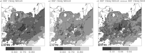
Table 4. Summary of results from previous studies investigating the impacts of changes in various components of the overall modeling system on estimates of RRFs for DM8H ozone

Study	Factors Considered	Typical Effect on RRF
Sistla et al.48	Photochemical model	≤0.04
	Emissions processor
Jones et al.47	Meteorological model	≤0.04
	Chemical mechanism
Hogrefe et al.44	Photochemical model	≤0.03
	Vertical mixing scheme
Koo et al.53	Updated natural emissions	≤0.04 (Estimated from Figure 7d, which reports percentage changes in average modeled seasonal fourth-highest DM8H ozone)
Kim et al.59	Physics parameterizations in MM5 Grid resolution	≤0.03
Study presented here	Biogenic emissions	0.06 (see Figure 6)

Impact of Biogenic Emission Differences on PM_2.5 Concentrations

In addition to the differences in gas-phase ozone pollutant concentrations discussed above, the differences in biogenic emissions are also expected to impact simulated PM_2.5 concentrations through direct and indirect pathways in multi-pollutant chemical transport models such as CMAQ. On the basis of the CMAQ version 4.7 aerosol module description in Napelenok et al.,56 Foley et al.,48 and Carlton et al.,57 the most direct impact of biogenic emissions on simulated PM_2.5 concentrations is expected to be through the formation of SOAs from isoprene and mono- and sesquiterpenes. However, there is also the possibility of indirect impacts on biogenic and anthropogenic SOA production because the yields from some indirect pathways are sensitive to ambient NO_x concentrations and acid levels, which in turn are impacted by the effects of biogenic isoprene and NO emissions on gas-phase chemistry. Finally, the impacts of different isoprene and NO emissions on gas-phase chemistry may also affect the formation of sulfate and nitrate aerosols because sulfate formation is sensitive to H₂O₂ and ozone concentrations whereas nitrate formation is sensitive to HNO₃ concentrations.58

Impact on CMAQ Estimates of PM_2.5 Constituents

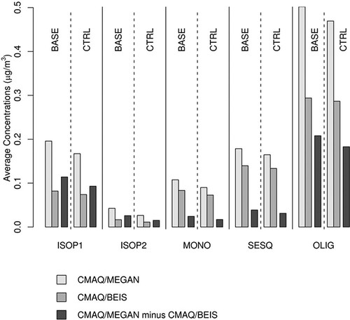
Figure 7 shows a bar chart of the seasonal average concentrations of various biogenic SOA components for BASE-MEGAN, BASE-BEIS, CTRL-MEGAN, and CTRL-BEIS as well as the differences between the MEGAN and BEIS simulations for the BASE and CTRL emission scenarios. For these bar charts, the concentrations were averaged over all nonwater grid cells. This figure presents the concentrations from the five pathways for the formation of biogenic SOA in CMAQ version 4.7 as described in Napelenok et al.,56 Foley et al.,48 and Carlton et al.57; namely, the two-product formation pathway from isoprene oxidation (ISOP1), the acid-catalyzed formation from isoprene (ISOP2), the formation pathways from the oxidation of monoterpenes (MONO) and sesquiterpenes (SESQ), and the oligomerization of aged particles from all biogenic sources (OLIG). For both platforms, the largest contribution to biogenic SOA comes from aged particles, whereas the second largest contribution differs between the MEGAN platform (formation from the two-product formation pathway from isoprene oxidation) and the BEIS platform (formation from the oxidation of SESQ). It can also be seen that the SOA concentrations are higher for the MEGAN platform than the BEIS platform for all species and scenarios, but that the differences between the MEGAN and BEIS results are lower for the CTRL compared with the BASE scenario. This may reflect reduced ozone and OH concentrations in the CTRL scenario, which would lead to reduced oxidation rates for isoprene, MONO, and SESQ.

Figure 7. Seasonal average concentrations of various biogenic SOA components for BASE-MEGAN, BASE-BEIS, CTRL-MEGAN, and CTRL-BEIS as well as the differences between the MEGAN and BEIS simulations for the BASE and CTRL emission scenarios. For these bar charts, the concentrations were averaged over all nonwater grid cells. This figure presents the concentrations from the five pathways for the formation of biogenic SOA in CMAQ version 4.7 as described in Napelenok et al.,56 Foley et al.,48 and Carlton et al.57; namely, the 2-product formation pathway from ISOP1, the acid-catalyzed formation from ISOP2, the formation pathways from the oxidation of MONO and SESQ, and the oligomerization of aged particles from all OLIG.

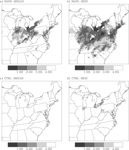
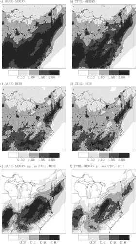
Figure 8 shows maps of the seasonal average biogenic SOA concentrations for BASE-MEGAN, BASE-BEIS, CTRLMEGAN, and CTRL-BEIS as well as the differences between the MEGAN and BEIS simulations for the BASE and CTRL emission scenarios. Here, the term “biogenic SOA” refers to the sum of SOA from the five pathways shown in Figure 7. In all scenarios, the highest average concentrations of biogenic SOA occur in the southern and southeastern portions of the modeling domain, areas that are characterized by high biogenic emissions of isoprene, MONO, and SESQ as shown in Figure 1. The biogenic SOA concentrations are up to 2 μg/m³ for the BASE-MEGAN scenario and up to 1.5 μg/m³ for the BASE-BEIS scenario. Consistent with Figure 7, for the BASE and CTRL scenarios, the BEIS platform yields lower biogenic SOA than the MEGAN platform by 0.1–0.7 μg/m³ throughout the domain. This is also consistent with the lower isoprene, monoterpene, and sesquiterpene emissions in BEIS and points to the important role of direct SOA formation from biogenic isoprene and terpene emissions. In addition, it can also be seen that the absolute concentrations and the platform differences are less for the CTRL than the BASE scenario, indicating the presence of nonlinear interactions between biogenic and anthropogenic emissions. As discussed above, this may reflect reduced ozone and OH concentrations in the CTRL scenario, which would lead to a reduced rate of isoprene, monoterpene, and sesquiterpene oxidation.

Figure 8. Maps of seasonal average biogenic SOA concentrations from the four model simulations and their differences: (a) BASE-MEGAN, (b) CTRL-MEGAN, (c) BASE-BEIS, (d) CTRL-BEIS, (e) BASE-MEGAN minus BASE-BEIS, and (f) CTRL-MEGAN minus CTRL-BEIS. All concentrations were averaged for May 15 to September 30, 2002 and are shown in units of μg/m³.

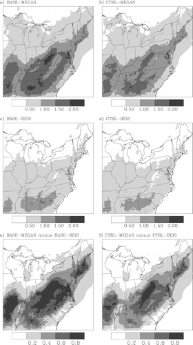
Figure 9 shows the corresponding results for total organic mass (OM), which is calculated as the sum of all 21 primary organic aerosol and SOA species simulated by CMAQ version 4.7. A comparison of corresponding panels in Figures 8 and 9 shows that biogenic SOA accounts for a large portion of total OM in the Southeast, whereas additional sources of OM are present in urban areas, especially the urban corridor from Washington, DC, to Boston, MA. Further analysis (results not shown) revealed that most of these additional contributions to total OM are from primary anthropogenic OM, the levels for which are the same for the BEIS and MEGAN simulations. The platform differences for OM (Figure 9, e and f) are almost identical to those for biogenic SOA (Figure 8, e and f), confirming that biogenic SOA is the major contributor to these differences and that the impact of the platform differences on total OM depends on the level of anthropogenic emissions and their interactions with biogenic emissions.

Figure 9. Maps of seasonal average total organic aerosol concentrations from the four model simulations and their differences: (a) BASE-MEGAN, (b) CTRL-MEGAN, (c) BASE-BEIS, (d) CTRL-BEIS, (e) BASE-MEGAN minus BASE-BEIS, and (f) CTRL-MEGAN minus CTRL-BEIS. All concentrations were averaged for May 15 to September 30, 2002 and are shown in units of μg/m³.

Relative Response to Anthropogenic Emission Reductions

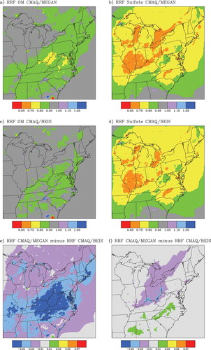
The results shown in Figures 8 and 9 indicate that CMAQ-simulated biogenic SOA and total OM predictions for both platforms are lower for the CTRL compared with the BASE scenario (i.e., the biogenic PM levels are responsive to anthropogenic emission reductions). Moreover, the differences for these pollutants between the MEGAN and BEIS platforms change between the BASE and CTRL scenario, implying that some of the PM_2.5 species simulated by the two platforms have different sensitivities to anthropogenic emissions reductions. As in the case for ozone, the current modeling guidance by EPA calls for the calculation of an RRF from a base year and future year modeling simulation39 to determine a future year regulatory value for annual or 24-hr PM_2.5 concentrations. The RRF calculation is performed for each of the major components of PM_2.5; namely, sulfate, nitrate, elemental carbon (EC), OM, and other primary PM_2.5. This analysis computed RRF on the basis of the average CMAQ-simulated May-to-September concentrations for total OM and sulfate for both platforms. RRFs for the other components were not calculated because they are not dependent on biogenic emissions (e.g., EC and other primary PM_2.5 are dependent on primary anthropogenic emissions) or constitute a very small portion of total PM_2.5 mass (e.g., the fraction of the nitrate portion of total PM_2.5 is very low based on measurements from the Federal Reference Method [FRM] for the study time period). It should be noted that an actual regulatory process analysis for the annual PM_2.5 National Ambient Air Quality Standards (NAAQS) requires that the RRF be estimated for each quarter, whereas the analysis presented here considers only RRF calculated from the May-to-September CMAQ simulations because this is the time period when differences in biogenic emissions would be expected to have their greatest impact on RRF estimates.

Figure 10 shows the maps of RRF calculations for OM and sulfate for MEGAN and BEIS and maps showing the differences in RRF between the two platforms. For total OM, the MEGAN platform shows lower RRF than the BEIS platform, indicating a greater response of total OM toward anthropogenic emission reductions (Figure 10, a, c, and e). This difference is most pronounced in the central portion of the modeling domain, which is characterized by relatively high biogenic emissions and significant reductions in anthropogenic NO_x emissions between the BASE and CTRL scenario. Because typical summer average OM concentrations estimated from FRM measurements following the EPA guidance document39 range from 2 to 5 μg/m³ in many areas of the modeling domain, RRF differences on the order of 0.05 as shown in Figure 10 would lead to estimated differences of the summer OM component of future year design values of 0.1–0.25 μg/m³. The RRF maps for sulfate (Figure 10, b and d) show values ranging from 0.65 to 0.8 for most of the modeling domain for both platforms. The absolute RRF differences for sul-fate between the platforms are less than 0.01 for most of the modeling domain (Figure 10f), but there is a tendency for the MEGAN platform to have a lower RRF (greater response) than the BEIS platform along the Ohio River Valley and its downwind areas as well as a small portion of the Northeast urban corridor, whereas there is a reverse tendency for the southeastern portions of the modeling domain where the BEIS platform tends to show a lower RRF (greater response) than the MEGAN platform. These differences again illustrate that the impact of different biogenic emissions is not limited to gas-phase pollutants such as ozone but can also affect the simulated response of PM_2.5 to anthropogenic emission reductions. Assuming that typical summer average sulfate concentrations estimated from FRM measurements are 4–8 μg/m³ in many areas of the modeling domain, RRF differences on the order of 0.02, as shown for some regions in Figure 10,would lead to estimated differences of the sulfate component of future year design values on the order of 0.1–0.15 μg/m³.

Figure 10. Maps of the dimensionless RRF for May-to-September average total organic aerosol mass and sulfate (SO₄) concentrations calculated for the MEGAN and BEIS platforms using the BASE and CTRL emission scenarios: (a) OM RRF for the MEGAN platform, (b) SO₄ RRF for the MEGAN platform, (c) OM RRF for the BEIS platform, (d) SO₄ RRF for the BEIS platform, (e) OM RRF for the MEGAN platform minus OM RRF for the BEIS platform, and (f) SO₄ RRF for the MEGAN platform minus SO₄ RRF for the BEIS platform.

CONCLUSIONS

This study characterized the impact of differences in biogenic emissions estimates from two current-generation biogenic emission modeling platforms, MEGAN and BEIS, on the CMAQ responses for ozone and PM_2.5 levels for a NO_x emission control scenario. For ozone, results confirmed the finding from previous studies that the impact of biogenic emission differences depends on the magnitude of anthropogenic NO_x emissions.2,5,7 The MEGAN-based platform used in this study showed a more NO_x- limited regime indicated by a higher H₂O₂/HNO₃ ratio in the base-case anthropogenic emissions scenario compared with the BEIS platform and consequently showed a larger absolute and relative ozone response to a hypothetical anthropogenic NO_x emission reduction scenario. Applying the current EPA modeling guidance procedure to typical maximum present-day daily maximum 8-hr ozone observed DVCs, the differences in future year design values stemming from biogenic emission differences were estimated to be on the order of 4 ppb or more, caused by RRF differences of 0.05 or more. As summarized in Table 4, this difference in RRF is larger than RRF differences introduced by differences in various other aspects of the overall modeling platform such as the meteorological model, emissions processor, or photochemical model.

For key secondary PM_2.5 species, the results show substantial differences in modeled concentrations when using different biogenic emission estimates in the base-case and emission control-case scenarios. Interpreting the effect in the context of the current regulatory framework for the annual PM_2.5 NAAQS, differences of the summer OM component of future year design values of 0.1 to 0.25 μg/m³ are found, corresponding to approximately 1–2% of the value of the annual PM_2.5 NAAQS set at 15 μg/m³. Furthermore, results show that the impacts of biogenic emission differences are not restricted to the organic portion of PM_2.5 but can also affect secondary inorganic species such as sulfate, albeit to a smaller extent. This highlights the complex interactions between gas-phase and aerosol chemistry in a multipollutant modeling framework that need to be considered when quantifying the impacts of emission uncertainties on regulatory modeling applications. More generally, the results presented in this study point to the need for further research aimed at reducing the uncertainties associated with estimating biogenic emissions and their transformation in the atmosphere.

ACKNOWLEDGMENTS

Support for this study was provided by the New York State Department of Environmental Conservation and the New Jersey Department of Environmental Protection. The viewpoints expressed in this work are solely the responsibility of the authors and do not necessarily reflect the views of the funding agencies or their contractors.

REFERENCES

- Chameides , W.L. , Lindsay , R.W. , Richardson , J. and Kiang , C.S . 1988 . The Role of Biogenic Hydrocarbons in Urban Photochemical Smog: Atlanta as a Case Study . Science , 241 : 1473 – 1475 .
- Fiore , A.M. , Horowitz , L.W. , Purves , D.W. , Levy , H. II , Evans , M.J. , Wang , Y. , Li , Q. and Yantosca , R.M. 2005 . Evaluating the Contribution of Changes in Isoprene Emissions to Surface Ozone Trends over the Eastern United States . J. Geophys. Res. , 110 doi: 10.1029/2004JD005485
- Kang , D.W. , Aneja , V.P. , Mathur , R. and Ray , J.D. 2003 . Nonmethane Hydrocarbons and Ozone in Three Rural Southeast United States National Parks: A Model Sensitivity Analysis and Comparison to Measurements . J. Geophys. Res. , 108 doi: 10.1029/2002JD003054
- Li , G.H. , Zhang , R.Y. , Fan , J.W. and Tie , X.X. 2007 . Impacts of Biogenic Emissions on Photochemical Ozone Production in Houston, Texas . J. Geophys. Res. , 112 doi: 10.1029/2006JD007924
- Pierce , T. , Geron , C. , Bender , L. , Dennis , R. , Tonnesen , G. and Guenther , A. 1998 . Influence of Increased Isoprene Emissions on Regional Ozone Modeling . J. Geophys. Res. , 103 : 25611 – 25629 .
- Roselle , S.J. , Pierce , T.E. and Schere , K.L. 1991 . The Sensitivity of Regional Ozone Modeling to Biogenic Hydrocarbons . J. Geophys. Res. , 96 : 7371 – 7394 .
- Roselle , S.J. 1994 . Effects of Biogenic Emission Uncertainties on Regional Photochemical Modeling of Control Strategies . Atmos. Environ. , 28 : 1757 – 1772 .
- von Kuhlmann , R. , Lawrence , M.G. , Poschl , U. and Crutzen , P.J. 2004 . Sensitivities in Global Scale Modeling of Isoprene . Atmos. Chem. Phys. , 4 : 1 – 17 .
- Bench , G. , Fallon , S. , Schichtel , B. , Malm , W. and McDade , C. 2007 . Relative Contributions of Fossil and Contemporary Carbon Sources to PM2.5 Aerosols at Nine Interagency Monitoring for Protection of Visual Environments (IMPROVE) Network Sites . J. Geophys. Res. , 112 D10205
- Brewer , P.F. and Adlhoch , J.P. 2005 . Trends in Speciated Fine Particulate Matter and Visibility across Monitoring Networks in the Southeastern United States . Journal of the Air & Waste Management Association , 55 : 1663 – 1674 .
- Kleindienst , T.E. , Jaoui , M. , Lewandowski , M. , Offenberg , J.H. , Lewis , C.W. , Bhave , P.V. and Edney , E.O. 2007 . Estimates of the Contributions of Biogenic and Anthropogenic Hydrocarbons to Secondary Organic Aerosol at a Southeastern US Location . Atmos. Environ. , 41 : 8288 – 8300 .
- Lewandowski , M. , Jaoui , M. , Kleindienst , T.E. , Offenberg , J.H. and Edney , E.O. 2007 . Composition of PM2.5 during the Summer of 2003 in Research Triangle Park, North Carolina . Atmos. Environ. , 41 : 4073 – 4083 .
- Weber , R.J. , Sullivan , A.P. , Peltier , R.E. , Russell , A. , Yan , B. , Zheng , M. , de Gouw , J. , Warneke , C. , Brock , C. , Holloway , J.S. , Atlas , E.L. and Edgerton , E. 2007 . A Study of Secondary Organic Aerosol Formation in the Anthropogenic-Influenced Southeastern United States . J. Geophys. Res. , 112 doi: 10.1029/2007JD008408
- Yu , S.C. , Dennis , R.L. , Bhave , P.V. and Eder , B.K. 2004 . Primary and Secondary Organic Aerosols over the United States: Estimates on the Basis of Observed Organic Carbon (OC) and Elemental Carbon (EC), and Air Quality Modeled Primary OC/EC Ratios . Atmos. Environ. , 38 : 5257 – 5268 .
- Tao , Z. , Larson , S.M. , Wuebbles , D.J. , Williams , A. and Caughey , M. 2003 . A Summer Simulation of Biogenic Contributions to Ground-Level Ozone over the Continental United States . J. Geophys. Res. , 108 doi: 10.1029/2002JD002945
- Lelieveld , J. , Butler , T.M. , Crowley , J.N. , Dillon , T.J. , Fischer , H. , Ganzeveld , L. , Harder , H. , Lawrence , M.G. , Martinez , M. , Taraborrelli , D. and Williams , J. 2008 . Atmospheric Oxidation Capacity Sustained by a Tropical Forest . Nature , 452 : 737 – 740 .
- Paulot , F. , Crounse , J.D. , Kjaergaard , H.G. , Kurten , A. , St. Clair , J.M. , Seinfeld , J.H. and Wennberg , P.O. 2009 . Unexpected Epoxide Formation in the Gas-Phase Photooxidation of Isoprene . Science , 325 : 730 – 733 .
- Paulot , F. , Crounse , J.D. , Kjaergaard , H.G. , Kroll , J.H. , Seinfeld , J.H. and Wennberg , P.O. 2009 . Isoprene Photooxidation: New Insights into the Production of Acids and Organic Nitrates . Atmos. Chem. Phys. , 9 : 1479 – 1501 .
- Archibald , A.T. , Jenkin , M.E. and Shallcross , D.E. An Isoprene Mechanism Intercomparison . Atmos. Environ. , in press
- Guenther , A. , Karl , T. , Harley , P. , Wiedinmyer , C. , Palmer , P.I. and Geron , C. 2006 . Estimates of Global Terrestrial Isoprene Emissions Using MEGAN (Model of Emissions of Gases and Aerosols from Nature) . Atmos. Chem. Phys. , 6 : 3181 – 3210 .
- Pierce , T.E. and Waldruff , P.S. 1991 . PC-BEIS—A Personal-Computer Version of the Biogenic Emissions Inventory System . Journal of the Air & Waste Management Association , 41 : 937 – 941 .
- Trainer , M. , Williams , E.J. , Parrish , D.D. , Buhr , M.P. , Allwine , E.J. , Westberg , H.H. , Fehsenfeld , F.C. and Liu , S.C. 1987 . Models and Observations of the Impact of Natural Hydrocarbons on Rural Ozone . Nature , 329 : 705 – 707 .
- Schwede , D. , Pouliot , G. and Pierce , T. Changes to the Biogenic Emission Inventory System Version 3 (BEIS3) . Presented at the 4th Annual CMAS Models-3 Users' Conference . Chapel Hill , NC .
- Warneke , C. , de Gouw , J.A. , del Negro , L. , Brioude , J. , McKeen , S. , Stark , H. , Kuster , W.C. , Goldan , P.D. , Trainer , M. , Fehsenfeld , F.C. , Wiedinmyer , C. , Guenther , A.B. , Hansel , A. , Wisthaler , A. , Atlas , E. , Holloway , J.S. , Ryerson , T.B. , Peischl , J. , Huey , L.G. and Hanks , A.T.C. 2010 . Biogenic Emission Measurement and Inventories: Determination of Biogenic Emissions in the Eastern United States and Texas and Comparison with Biogenic Emission Inventories . J. Geophys. Res. , 115 doi: 10.1029/2009JD012445
- Niinemets , Ü. , Monson , R.K. , Arneth , A. , Ciccioli , P. , Kesselmeier , J. , Kuhn , U. , Noe , S.M. , Peñuelas , J. and Staudt , M. 2010 . The Leaf-Level Emission Factor of Volatile Isoprenoids: Caveats, Model Algorithms, Response Shapes and Scaling . Biogeosciences , 7 : 1809 – 1832 .
- Pinto , D. , Blande , J. , Souza , S. , Nerg , A.-M. and Holopainen , J. 2010 . Plant Volatile Organic Compounds (VOCs) in Ozone (O3) Polluted Atmospheres: The Ecological Effects . J. Chem. Ecol. , 36 : 22 – 34 .
- Baker , K. 2006 . Appendix H—Modeling Protocol Addendum: Technical Details , Rosemont , IL : Lake Michigan Air Directors Consortium, Midwest Regional Planning Organization .
- 2007 . Draft Modeling Technical Support Document , Washington , DC : Ozone Transport Commission .
- 2007 . The North Carolina 8-Hour Ozone Attainment Demonstration for the Charlotte-Gastonia-Rock Hill, NC-SC 8-Hour Ozone Nonattainment Area, Pre-Hearing Draft , Raleigh , NC : North Carolina Department of Environment and Natural Resources; Division of Air Quality .
- Vukovich , J.M. and Pierce , T. The Implementation of BEIS3 within the SMOKE Modeling Framework . Presented at the 11th International Emission Inventory Conference . Atlanta , GA
- CMAS SMOKE v2.5 Release Notes http://www.smoke-model.org/version2.5/html/Release_Notes_v25.html (http://www.smoke-model.org/version2.5/html/Release_Notes_v25.html) (Accessed: 2010 ).
- Byun , D. and Schere , K.L. 2006 . Review of the Governing Equations, Computational Algorithms, and Other Components of the Models-3 Community Multiscale Air Quality (CMAQ) Modeling System . Appl. Mech. Rev. , 59 : 51 – 77 .
- Byun , D.W. and Ching , J.K.S. 1999 . Science Algorithms for the EPA Models-3 Community Multiscale Air Quality (CMAQ) Modeling System , Research Triangle Park , NC : U.S. Environmental Protection Agency; National Exposure Research Laboratory . EPA/600/R-99/ 030
- 2009 . User's Guide to the Comprehensive Air Quality Model with Extensions (CAMx) Version 5.10 , Novato , CA : ENVIRON International Corporation .
- Horowitz , L.W. , Fiore , A.M. , Milly , G.P. , Cohen , R.C. , Perring , A. , Wooldridge , P.J. , Hess , P.G. , Emmons , L.K. and Lamarque , J.F. 2007 . Observational Constraints on the Chemistry of Isoprene Nitrates over the Eastern United States . J. Geophys. Res. , 112 doi: 10.1029/2006JD007747
- Wu , S. , Mickley , L.J. , Jacob , D.J. , Logan , J.A. , Yantosca , R.M. and Rind , D. 2007 . Why Are There Large Differences between Models in Global Budgets of Tropospheric Ozone? . J. Geophys. Res. , 112 doi: 10.1029/ 2006JD007801
- Zhang , Y. , Huang , J.P. , Henze , D.K. and Seinfeld , J.H. 2007 . Role of Isoprene in Secondary Organic Aerosol Formation on a Regional Scale . J. Geophys. Res. , 112 doi: 10.1029/2007JD008675
- Pouliot , G. A Tale of Two Models: A Comparison of the Biogenic Emission Inventory System (BEIS3.14) and Model of Emissions of Gases and Aerosols from Nature (MEGAN 2.04) . Presented at the 7th Annual CMAS Conference . Chapel Hill , NC .
- 2007 . Guidance on the Use of Models and Other Analyses for Demonstrating Attainment of Air Quality Goals for Ozone, PM2.5, and Regional Haze , Research Triangle Park , NC : U.S. Environmental Protection Agency . EPA-454/B-07-002
- Grell , G.A. , Dudhia , J. and Stauffer , D.R. 1994 . A Description of the Fifth-Generation Penn State/NCAR Mesoscale Model (MM5) , Boulder , CO : National Center for Atmospheric Research . Technical Note NCAR/TN-398 1 STR
- Kain , J.S. and Fritsch , J.M.. 1993 . Convective Parameterization for Mesoscale Models: The Kain–Fritsch Scheme. Cumulus Parameterization . Meteorol. Monograph. Am. Meteorol. Soc. , 46 : 165 – 170 .
- Dudhia , J. 1989 . Numerical Study of Convection Observed during the Winter Monsoon Experiment Using a Mesoscale Two-Dimensional Model . J. Atmos. Sci. , 46 : 3077 – 3107 .
- Zhang , D.-L. 1989 . The Effect of Parameterized Ice Microphysics on the Simulation of Vortex Circulation with a Mesoscale Hydrostatic Model . Tellus A , 41 : 132 – 147 .
- Zhang , D. and Anthes , R.A. 1982 . A High-Resolution Model of the Planetary Boundary Layer—Sensitivity Tests and Comparisons with SESAME-79 Data . J. Appl. Meteorol. , 21 : 1594 – 1609 .
- Zhang , D.L. and Zheng , W.Z. 2004 . Diurnal Cycles of Surface Winds and Temperatures as Simulated by Five Boundary Layer Parameterizations . J. Appl. Meteorol. , 43 : 157 – 169 .
- Dudhia , J. A Multi-Layer Soil Temperature Model for MM5 . Presented at the 6th Annual MM5 Users Workshop . Boulder , CO : National Center for Atmospheric Research .
- Otte , T.L. and Pleim , J.E. 2009 . The Meteorology-Chemistry Interface Processor (MCIP) for the CMAQ Modeling System . Geosci. Model Dev. Discuss. , 2 : 1449 – 1486 .
- Foley , K.M. , Roselle , S.J. , Appel , K.W. , Bhave , P.V. , Pleim , J.E. , Otte , T.L. , Mathur , R. , Sarwar , G. , Young , J.O. , Gilliam , R.C. , Nolte , C.G. , Kelly , J.T. , Gilliland , A.B. and Bash , J.O. 2009 . Incremental Testing of the Community Multiscale Air Quality (CMAQ) Modeling System Version 4.7 . Geosci. Model Dev. Discuss. , 2 : 1245 – 1297 .
- Hogrefe , C. , Civerolo , K.L. , Hao , W. , Ku , J.Y. , Zalewsky , E.E. and Sistla , G. 2008 . Rethinking the Assessment of Photochemical Modeling Systems in Air Quality Planning Applications . Journal of the Air & Waste Management Association , 58 : 1086 – 1099 . doi: 10.3155/1047-3289.58.8.1086
- Pouliot , G. and Pierce , T. Integration of the Model of Emissions of Gases and Aerosols from Nature (MEGAN) into the CMAQ Modeling System . Presented at the 18th International Emission Inventory Conference . Baltimore , MD .
- Houyoux , M.R. , Vukovich , J.M. , Coats , C.J. , Wheeler , N.J.M. and Kasibhatla , P.S. 2000 . Emission Inventory Development and Processing for the Seasonal Model for Regional Air Quality (SMRAQ) Project . J. Geophys. Res. , 105 : 9079 – 9090 .
- Kuhn , U. , Andreae , M.O. , Ammann , C. , Araújo , A.C. , Brancaleoni , E. , Ciccioli , P. , Dindorf , T. , Frattoni , M. , Gatti , L.V. , Ganzeveld , L. , Kruijt , B. , Lelieveld , J. , Lloyd , J. , Meixner , F.X. , Nobre , A.D. , Pöschl , U. , Spirig , C. , Stefani , P. , Thielmann , A. , Valentini , R. and Kesselmeier , J. 2007 . Isoprene and Monoterpene Fluxes from Central Amazonian Rainforest Inferred from Tower-Based and Airborne Measurements, and Implications on the Atmospheric Chemistry and the Local Carbon Budget . Atmos. Chem. Phys. , 7 : 2855 – 2879 .
- Koo , B. , Chien , C.-J. , Tonnesen , G. , Morris , R. , Johnson , J. , Sakulyanontvittaya , T. , Piyachaturawat , P. and Yarwood , G. 2010 . Natural Emissions for Regional Modeling of Background Ozone and Particulate Matter and Impacts on Emissions Control Strategies . Atmos. Environ. , 44 : 2372 – 2382 .
- Tonnesen , G.S. and Dennis , R.L. 2000 . Analysis of Radical Propagation Efficiency to Assess Ozone Sensitivity to Hydrocarbons and NOx: 2. Long-Lived Species as Indicators of Ozone Concentration Sensitivity . J. Geophys. Res. , 105 : 9227 – 9241 .
- Zhang , Y. , Vijayaraghavan , K. , Wen , X.Y. , Snell , H.E. and Jacobson , M.Z. 2009 . Probing into Regional Ozone and Particulate Matter Pollution in the United States: 1. A 1 Year CMAQ Simulation and Evaluation Using Surface and Satellite Data . J. Geophys. Res. , 114 doi: 10.1029/ 2009JD011898
- Napelenok , S.L. , Carlton , A.G. , Bhave , P.V. , Sarwar , G. , Pouliot , G. , Pinder , R.W. , Edney , E.O. and Houyoux , M. Updates to the Treatment of Secondary Organic Aerosols in CMAQv4.7 . Presented at the 7th Annual CMAS Conference . Chapel Hill , NC .
- Carlton , A.G. , Bhave , P.V. , Napelenok , S.L. , Pinder , R.W. , Sarwar , G. , Pouliot , G.A. and Edney , E.O. 2009 . Improved Treatment of Secondary Organic Aerosol in CMAQ . Environ. Sci. Technol. , submitted for publication
- Unger , N. , Shindell , D.T. , Koch , D.M. and Streets , D.G. 2006 . Cross Influences of Ozone and Sulfate Precursor Emissions Changes on Air Quality and Climate . Proc. Natl. Acad. Sci. USA , 103 : 4377 – 4380 .
- Kim , Y. , Fu , J.S. and Miller , T.L. 2010 . Improving Ozone Modeling in Complex Terrain at a Fine Grid Resolution. Part II: Influence of Schemes in MM5 on Daily Maximum 8-h Ozone Concentrations and RRFs (Relative Reduction Factors) for SIPs in the Non-Attainment Areas . Atmos. Environ. , 44 : 2116 – 2124 .