Using a Chemistry Transport Model to Account for the Spatial Variability of Exposure Concentrations in Epidemiologic Air Pollution Studies

ABSTRACT

Environmental epidemiology and more specifically time-series analysis have traditionally used area-averaged pollutant concentrations measured at central monitors as exposure surrogates to associate health outcomes with air pollution. However, spatial aggregation has been shown to contribute to the overall bias in the estimation of the exposure-response functions. This paper presents the benefit of adding features of the spatial variability of exposure by using concentration fields modeled with a chemistry transport model instead of monitor data and accounting for human activity patterns. On the basis of county-level census data for the city of Paris, France, and a Monte Carlo simulation, a simple activity model was developed accounting for the temporal variability between working and evening hours as well as during transit. By combining activity data with modeled concentrations, the downtown, suburban, and rural spatial patterns in exposure to nitrogen dioxide, ozone, and PM_2.5 (particulate matter [PM] ≤ 10 μm in aerodynamic diameter) were captured and parametrized. Exposures predicted with this model were used in a time-series study of the short-term effect of air pollution on total nonaccidental mortality for the 4-yr period from 2001 to 2004. It was shown that the time series of the exposure surrogates developed here are less correlated across co-pollutants than in the case of the area-averaged monitor data. This led to less biased exposure-response functions when all three co-pollutants were inserted simultaneously in the same regression model. This finding yields insight into pollutant-specific health effects that are otherwise masked by the high correlation among co-pollutants.

IMPLICATIONS

The methodology developed in this study suggests that spatially resolved pollutant concentrations combined with demographic data may be used in a parametric way in an epidemiological time-series study and provide additional information on the spatial variability of exposure. The principal advantage of the method is that the time series of the exposure surrogates used in the regression against health outcomes are less correlated among co-pollutants. It is therefore possible to estimate statistically significant associations between each co-pollutant and the health outcome and thus distinguish the corresponding health effects.

INTRODUCTION

There is a long history of epidemiology research on the relationship between spatial and temporal variability in ambient concentrations and health outcomes,1 including acute and chronic effects of particulate and gaseous air pollutants on morbidity and mortality.2–5 Although the specific study design and health endpoint may vary among different environmental epidemiology studies, in most cases ambient concentrations from central monitors are aggregated over the geographical area of the study to a single exposure surrogate.6,7 The assumption in these studies is that the mean of the personal exposures over the study population may be considered to be sufficiently correlated to this area-averaged exposure metric if the selected monitor data satisfy certain conditions.8

However, several shortcomings of the spatial aggregation of ambient concentrations have been put in evidence, especially over urban areas, where various types of emitting sources coexist over relatively short distances. Recent research of the Health Effects Institute on the health effects of traffic-related air pollution showed that the zones most impacted by traffic-related pollution are up to 300–500 m from highways and other major roads, and when calculated for large cities in North America that would include 30–45% of the population.9 In most cases, only a few monitoring stations are available inside of cities. For gaseous species such as ozone (O₃) and nitrogen dioxide (NO₂), the concentration fields of which are highly heterogeneous in space, aggregating concentrations over a few monitors yields inadequate surrogates of the actual mean of personal exposures.

Another problem arising in the time-series analysis because of spatial aggregation of ambient concentrations is the inability to differentiate the health effects of multiple correlated pollutants.10,11 The use of collocated measurements leads to high correlations among the time series of primary pollutants emitted from the same type of sources (e.g., traffic NO_x and PM emission). If the correlation among the time series of co-pollutants is higher than the correlation between a specific pollutant and the corresponding “true” personal exposure, the overall health effect is typically masked by the pollutant with the best representation from the monitor network and it is impossible to further separate the relative impact of each co-pollutant.12 The estimation may be biased toward or away from zero in a multiple-pollutant regression model depending on the direction and magnitude of the correlation between exposure prediction error and exposure surrogate.13,14 Thus, positive associations may be found for an “innocent” species if it is correlated with another toxic species accounted for in the same multiple-pollutant model.

The analysis presented here examines how accounting for the spatial variability of exposure by using spatially resolved concentration fields from air quality modeling and accounting for population activity may decrease exposure misclassification in the health study. The main advantages of using modeled concentrations are the larger spatial coverage and variability in model output compared with monitor data as well as the simultaneous representation of multiple pollutants. The second part of the exposure module developed for this study uses demographic information based on county-level census data and applies a three-level activity pattern dividing daily exposures into working hours, evening hours, and exposure during transit from home to work and vice versa. Although this activity model is based on rough assumptions (e.g., homogeneous time frames defining work and evening hours across the population and transit duration being deduced from mean distances between the centroids of the work and residence county polygons), it is still a refinement compared with the common assumption of homogeneous exposure across space and time. These simplifications made it possible to run long-period simulations (necessary for the epidemiological application) and test the sensitivity of the results under several modeling configurations. This is very important because before developing a complex exposure model (a highly consuming calculation in terms of central processing unit [CPU] and computation time), one should test for what the key parameters are with respect to the state-of-the-art epidemiological applications.

The use of model predictions instead of monitor data suffers from uncertainties related to the modeling system, especially considering that air quality model outputs are used in this application in a spatially and temporally resolved way. Further adjustments have to be applied on model raw output to assign exposure in a more accurate way. Krigging or land-use regression methods have been used in previous exposure assessment studies.15–17 This study used the recently developed subgrid-scale module that accounts for small-scale emission variability and assigns ambient concentrations in subgrid environments such as on roads or in residential areas or parks.18

The goal of this study is therefore twofold: First, the issue of the exposure's spatial variability over the urban environment is addressed; next, this information is used in a Poisson regression to study short-term associations between simultaneous exposure to three pollutants (O₃, NO₂, and PM_2.5 [particulate matter ≤ 2.5 μm in aerodynamic diameter) and mortality. These particular pollutants were chosen because previous epidemiological research has already established their short-term effects on mortality in the same context. Also, this previous epidemiology research19,20 can be used as a point of reference to study how the incorporation of the new exposure dataset influences the estimation of the exposure-response functions.

METHODS AND DATA

Air Quality Modeling

This study focuses on the greater Paris region (1.25–3.58° east, 47.89–49.45° north) with a population of approximately 11,700,000 people, of which more than 2 in the city of Paris. The area is situated away from the coast and is characterized by uniform and low topography.

Under anticyclonic conditions, polluted air from northern Europe enters the study domain. Enhanced photochemical activity is favored by sunlight, leading to persisting O₃ plumes, especially in summer.21 Ambient O₃, NO₂, and PM_2.5 concentrations were estimated with the Eulerian multiscale chemical transport model (CTM) CHIMERE (http://www.lmd.polytechnique.fr/chimere/) from January 1, 2001 to December 31, 2004. The modeling domain consists of a coarse resolution grid over Western Europe from 10° west to 22° east and 35–57° north with a 0.5° horizontal resolution providing boundary conditions to the fine resolution nest over the Paris region. The nest covers an area of 160 × 130 km² with 53 zonal and 43 meridional cells at the first vertical layer at a 3- by 3-km grid resolution. On the vertical, the domain is divided into 10 layers from the ground to 500 hPa. The model has been thoroughly evaluated for this region on a long-term basis with routine air quality network measurements (O₃, nitric oxide [NO], NO₂, particulate matter) and with observations from the ESQUIF campaign.22

Chemical boundary conditions for the coarse resolution simulation are driven by GOCART model monthly climatologies for aerosol species23 and by the LMDz-INCA global chemical weather forecast system for gas-phase species.24–26

Dynamic calculations were provided by the nonhydrostatic Weather Research and Forecasting (WRF) model (version 3; http://www.wrf-model.org). The model is run at three-level, two-way nested grids at horizontal resolutions of 45, 15, and 5 km with 31 vertical layers from the surface (i.e., 900 hPa) to 100 hPa. Initial and lateral boundary conditions for the meteorological simulations were obtained from 6-hr analyses from the National Centers for Environmental Protection (NCEP) Global Final (FNL) at a resolution of 1°. The WRF model uses the Yonsei University (YSU) planetary boundary layer (PBL) scheme27 and the Noah Land Surface model scheme28 with soil temperature and moisture in four layers, fractional snow cover, and frozen soil physics that provide heat and moisture fluxes for the PBL.

Anthropogenic emissions for the regional domain (3-km resolution grid) are provided by the 1-km regional inventory developed by AIRPARIF (http://www.airparif.asso.fr) for the ESMERALDA project (http://www.esmeralda-web.fr). The elaboration of the inventory follows the European conventions on annual datasets of surface emissions based on a bottom-up approach for air quality forecasts. It considers oxides of nitrogen (NO_x), speciated volatile organic compounds, sulfur dioxide (SO₂), carbon monoxide (CO), PM₁₀ (particulate matter ≤ 10 μm) and PM_2.5 from fixed industrial sources, mobile sources, and biogenic sources. Emissions for the European domain (coarse resolution) are taken from the European Monitoring and Evaluation Programme (EMEP) inventory (http://www.emep.int).

The 3- by 3-km CTM resolution cannot resolve concentration gradients close to emission sources.29,30 Never theless, human activity and exposure take place at a fine scale, which is typically represented by an administrative unit such as census tracts. To overcome this, special emission treatment is implemented in the model: Transferring the subgrid-scale variability of surface emissions to concentration variability, subgrid or “local source-specific” concentrations are estimated along with the standard grid-averaged or “regional background.”18 Grid cells are divided into four types of source-specific subgrid areas: (1) on-road, (2) residential, (3) parks, and (4) all other sources. Over each subgrid surface, only emissions of the corresponding sources are considered. The CTM simulation is split at each model time step into separate computations over each one of these four surfaces, yielding source-specific concentration components. The advantage of this implementation is that in addition to the usual grid-averaged concentration provided by the CTM, complementary information concerning its variability is obtained because of heterogeneous surface emissions over the unresolved subgrid scale.

Demographic Data

County-level census data were provided by the French National Institute for Statistics and Economic Studies (INSEE; http://www.insee.fr/en/) for the eight counties of the Paris region (Table 1). On the basis of population density the Parisian population was divided into “downtown” (county 75), “suburban” (counties 92, 93 and 94), and “rural” groups (counties 77, 78, 91, and 95) (Figure 1b). As shown in Table 1, the largest part of the daily intraregional travel involves the downtown and suburban areas. A mean fraction of 10% of the residents of the suburban area work downtown and a similar fraction of the downtown population works in the suburbs. The fraction of the rural population working downtown is only 5%, with most of the population working inside of the county of residence (∼75%). A very low variability is observed in the nonworking population fraction across counties (∼33%).

Table 1. Population distribution among the eight counties of the greater Paris region provided by INSEE

County Name/Number	Residents ^a (%)	Workers (%) ^b	Residents Working Outside (%) ^c	Workers Living Inside (%) ^d	Inactive Population (%) ^e
Paris/75 ^f	19.4	26.8	14.6	13.0	36.2
Hauts-de-Seine/92 ^g	13.1	16.5	14.1	7.3	29.1
Seine-Saint-Denis/93 ^g	12.6	11.3	15.1	3.2	31.1
Val-de-Marne/94 ^g	11.2	10.4	13.3	3.0	30.2
Seine-et Marne/77 ^h	10.9	8.5	10.1	1.1	36.9
Yvelines/78 ^h	12.4	9.9	11.1	1.9	36.9
Essone/91 ^h	10.4	8.5	10.1	1.5	34.0
Val-d'Oise/95 ^h	10.1	8.1	114	1.5	31.9
Notes: Distribution of the ∼11,000,000 individuals according to their place of ^aresidence and ^bwork; ^cFraction of each county's residents working outside of the county; ^dFraction of each county's workers living in a different county than work; ^eInactive fraction of each county's residents; ^fDowntown, ^gsuburban, and ^hrural classification.

Figure 1. Maps of the greater Paris region with the boundaries of the eight counties representing the downtown district (county 75), the suburban area (counties 92, 93, and 94) and the rural area (counties 77, 78, 91, and 95). (a) CHIMERE model grid with points representing the centers of 53 zonal and 43 meridional cells at equal distances of 3 km. (b) Population density (number of residents/km², also shown are mean density values for each county). Shown area covers 160 × 130 km².

Exposure Event Sequences

To simulate personal outdoor exposure concentrations (called “OECs” to avoid confusion with simple concentration data), a Monte Carlo simulation was set up that respects the aforementioned demographical distributions but has the additional advantage of following individuals from a sample population of 100,000 along with their daily intraregional travel from home to work. A three-activity diary was created for each member of the Monte Carlo simulation that defined the time segments spent by each individual at each one of the three different environments involved in this study (residence, work, and on-road or in transit). For a typical 24-hr day, one time interval of exposure at the area of residence is considered from 7:00 + δt p.m. to 8:00 a.m. and a second time interval for exposure at the work place takes place from 8:00+δt a.m. to 7:00 p.m. δt is a time segment accounting for the morning and evening transit between home and work at weekdays and it is calculated based on the distance between the centroids of the polygons defining county boundaries: 90 min for transit between rural and urban areas, 60 min between rural and suburban areas as well as between suburban and downtown, and 30 min of commute time if residence and work places are in the same county. These assumptions are based on data provided from INSEE studies showing that this time schedule applies to most of the French working population. During transit, on-road concentration levels are computed with the subgrid-scale emissions module implemented in the CTM (see Air Quality Modeling section). During weekends and holidays, people are assumed to stay within their residence area, and a 30-min commute time is assigned to all individuals considering transportation for various reasons (shopping, etc.). The same assumption also applies to the inactive part of the population during weekdays.

It should be mentioned here that the activity diaries generated by this simplified model are based on rough assumptions: The same start time and end time of work days are assigned to all work-wise active individuals, and the only allowed variability is across county and ranges from 30 to 90 min depending on the distance between residence and work counties. Transportation modes are not accounted for in the model, and during transit all individuals are supposed to be exposed to on-road pollution. No infiltration indoors is considered and therefore all exposure levels refer to outdoor ambient modeled concentrations. To avoid adding uncertainties due to air quality model error at fine resolution, the intracounty variability of pollutant concentrations was treated in a stochastic manner through the Monte Carlo simulation. This also explains the choice to use county-level census data instead of finer demographic information such as census tract or census block, for which the spatial scale is comparable to the air quality model resolution and would demand explicit treatment. It should be noted that even under the assumption of homogeneous activity among the population, the development of exposure surrogates for this study is still a refinement compared with what is used in most health studies, in which no population activity is taken into consideration at all.19,20

Concentration levels during each one of the three exposure intervals are calculated with the CTM and then, for each member of the Monte Carlo simulation, they are weighted with the corresponding exposure time intervals of the three-activity diary. Considering the three-activity diary used here, the general expression of exposure is given by

(1)

where OEC represents the daily averaged personal exposure concentrations; c _res(t), c _wrk(t), and c _trf(t) are the modeled concentrations at the corresponding grid cell at hour t; and t _res, t _wrk, and t _trf are the temporal intervals of exposure at home, work, and traffic (near roads), respectively. Given the small number of degrees of freedom of the problem (i.e., place of residence, place of work, and working activity), the distribution of the final output dataset converges at a relatively low population of 100,000 members (∼1% of the population of the Paris region) (Figure 2).

Figure 2. Population-averaged OEC estimates as a function of the total number of the members of the Monte Carlo simulation showing the convergence of the simulation to a stable OEC dataset. The error is calculated relative to OEC estimates for an ensemble of 200,000 members.

SPATIAL VARIABILITY OF OECS

Distribution of Exposure

Four-year OEC data (2001–2004) are estimated with the described methodology. The time series of these estimates for O₃, NO₂, and PM_2.5 and for all of the members of the Monte Carlo simulation are shown in the two-dimensional histograms of Figure 3. The distribution of OEC data among the population presents a trimodal structure throughout the simulation period for all three pollutants. These three modes show the following trends:

Figure 3. Four-year time series of OEC distribution (2001–2004) for (a) O₃, (b) NO₂, and (c) PM_2.5. Color code corresponds to the number of individuals exposed to a given concentration level (vertical axis).

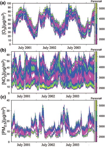
•	The high-exposure mode is more clearly distinguishable for O3 and NO2 than for PM2.5. This exposure mode is particularly highly populated in summer for O3.
•	The medium-exposure mode covers a larger part of the OEC spectrum for O3 and NO2 than the other two modes (high and low). This mode often overlaps with the high-exposure mode for PM2.5. The low-exposure mode is more narrow than the medium-exposure mode but is highly populated, especially for NO2.

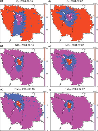
The presence of three distinct exposure modes shows that the distribution of exposure is not uniform among the population. As shown in Figure 3, low- and high-exposure modes may deviate from the medium mode by 75%. This stresses the need to represent this variability into an epidemiologic model. The trimodal structure of the OEC distribution raises the question of whether it is possible to associate each exposure mode with specific groups of the population. To answer this, the daily OEC estimates of all of the inhabitants of the same air quality grid cell were averaged to obtain the spatial distribution of modeled exposure concentrations. Two examples of this representation of the OEC data are given by the surface maps of a winter day (February 15, 2004) and a summer day (July 7, 2004) (Figure 4). In both examples, the spatial distribution of exposure concentrations also presents a trimodal aspect following a downtown, suburban, and rural pattern. Downtown is characterized by lower exposure to O₃ compared with the medium-exposure levels modeled over the suburbs and the high-exposure levels in the rural area due to photooxidant formation. For primary species such as NO_x and PM, exposure modes are directly linked to the spatial distribution of emissions. The highest exposures are modeled downtown, where the largest part of traffic activity takes place.

Figure 4. Surface maps of daily averaged exposures to (a, b) O₃, (c, d) NO₂, and (e, f) PM_2.5. Color code corresponds to exposure levels expressed in μg/m³. Maps on the left represent a winter day (February 15, 2004), and maps on the right represent a summer day (July 7, 2004).

To quantify these observations, a mixture-distribution model was proposed to fit to the 4-yr modeled exposure concentrations and link the three dominant modes of the exposure distribution (low, medium, and high) to the downtown, suburban, and rural population groups. The representation of population exposure via a parametric distribution is not a new concept.31,32 However, both of the mentioned studies suggest a single, lognormal distribution to fit to their data. Given the trimodal structure of the exposure distribution, a summation model is proposed that is comprised of three normal distributions for the parameterization (3-Gauss summation model hereafter):

(2)

where x is the exposure concentration μg m³); μ_i and σ_i are the mean and variance of each distribution, respectively; and f _i is the relative weight coefficient (RWC) of each distribution in the composite formula. RWCs represent the fractions of the population exposed to each mode of the distribution.

Parameterization

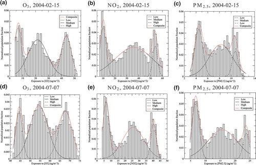
The three sets of mean, variance, and RWC data are treated as unknown parameters for the multivariate nonlinear fit. The result of the parameterization is a 4-yr time series for each one of the nine parameters (three sets of three parameters). Figure 5 shows the result of the fit to the OEC distribution for two days—the same days chosen for the representation of OEC spatial distribution through surface maps (Figure 4). For both cases and for all three pollutants, the 3-Gauss summation model is able to correctly represent the distribution of OEC data (histograms). Here it is noted that the ranges of each mode of the composite distribution of Figure 5 match with the ranges of the three exposure modes identified on the surface maps of Figure 4 for all three pollutants and both days. On days when the trimodal model was found to be inappropriate to fit to the distribution of exposure predictions, the authors attempted to fit a bimodal or mononormal distribution model over the OEC dataset. In practice, a criterion was imposed based on the distance between the maxima of the three individual distributions of the 3-Gauss summation model: If the fit converges in a composite distribution for which the difference between the means of two consecutive distributions is lower than 20% of the variance of either of the distributions, the two distributions are merged into a single one. For example, this case occurs on days when long-range transport brings a highly polluted air mass inside of the entire domain of the study or on days of high photooxidant activity in which the O₃ concentration is high all over the region. On such days, the exposure is rather normally distributed and a single Gaussian distribution fits better to exposure predictions. The former case occurred approximately 5% of the time, whereas the latter occurred approximately 1% of the time for the three pollutants. Given the low number of cases and to avoid discontinuities in the time series of the parameters of the distributions, the “vanishing” modes were not removed. Mean RWC ratios were calculated from the rest of the parameterization and were used to share the data of the binormal or mononormal distributions in three Gaussian parts. In the bimodal case, it was considered that the distribution with the largest variance corresponds to the medium-exposure mode, and then it was split into two distributions with the same means and variances for the respective fixed RWC ratio. In the mononormal distribution fit, all data were shared in three distributions with the same means and variances according to the mean RWC ratios.

Figure 5. Two-day example of the result of the fit of the trimodal distribution model on the OEC data (histograms) for (a, d) O₃, (b, e) NO₂, and (c, f) PM_2.5, with the red line showing the parametrized composite distribution and the black lines illustrating the intermediate fit of single Gaussian distributions on each one of the three modes of the distribution. Graphs on the top represent a winter day (February 15, 2004), and maps on the bottom represent a summer day (July 7, 2004).

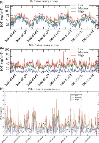
The time series of the means of the three normal distributions fitted to each mode of the OEC data distribution are shown in Figure 6. The time series were smoothed with a 7-day moving average to filter out short-term fluctuations. The three modes are clearly distinguishable throughout the period of the study for the three pollutants. The means of the three exposure modes for O₃ follow a seasonal cycle with higher exposures during summer than during winter. The seasonal trend is much less pronounced for NO₂ and PM_2.5. For all three pollutants, the means of the high- and low-exposure modes deviate from the medium-exposure mode by more than 50%, showing once more the potential benefits of taking into account the heterogeneity of exposure among the population in health studies.

Figure 6. Time series of the parametrized means of the (red) high-, (green) medium-, and (blue) low-exposure modes of (a) O₃, (b) NO₂, and (c) PM_2.5. A 7-day moving average filter is used to smooth out short-term fluctuations.

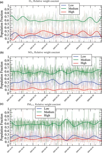
RWC (f _i) corresponds to the fraction of the population exposed to the ith mode. Figure 7 shows the evolution of these three coefficients through time. The time series of RWCs were decomposed in different time scales with wavelet decomposition. The signal was then reconstructed after filtering out the time scales with periods shorter than 6 mo. Only interseasonal fluctuations are therefore represented in Figure 7, which allows for comparison of the relative weight of the three exposure modes over long time scales. For the three pollutants, more than 60% of the population is exposed to the medium-exposure mode all year long. For NO₂ and PM_2.5, the fraction of the population exposed to the low- and medium-exposure modes fluctuates around 30%; a strong negative correlation is also noted between the RWCs of the low- and medium-exposure modes. This is a sign of people moving between these two exposure modes as a function of time. The lowest RWCs are observed for the high-exposure mode for NO₂ and PM_2.5, with values ranging around 10%. For O₃, an intra-annual movement of people is observed between the high- and medium-exposure modes, with the corresponding RWC values ranging around 20 and 70%, respectively. During the summer, the relative importance of the high-exposure mode increases compared with the lower RWC observed for this O₃ exposure mode during winter.

Figure 7. Time series of the parametrized RWCs showing the fractions of the population exposed to the (red) high-, (green) medium-, and (blue) low-exposure modes of (a) O₃, (b) NO₂, and (c) PM_2.5. Fine lines represent daily variations, whereas thick lines show the result of a low-pass filter over the data in which only seasonal variations are represented. Short-term variability is smoothed out by means of wavelet decomposition.

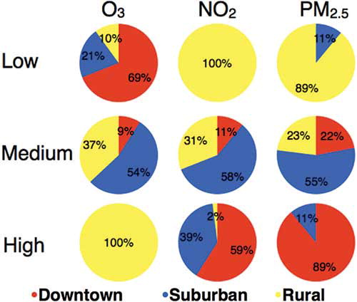
The demographic composition of each exposure mode was quantified in downtown, suburban, and rural populations by distributing OEC data back to each exposure mode for the whole period of the study as shown in Figure 8. The downtown and rural populations dominate the low- and high-exposure modes, whereas the medium exposure mode is more heterogeneous with the principal suburban component (>50% of its population) being mixed with nonnegligible downtown and rural fractions. This heterogeneity is presumably due to population movement between downtown and rural areas mixing high- and low-pollutant concentration levels in the daily averaged exposure burden. This shows the importance of taking into account activity patterns in the estimation of exposure. If the concentration was only combined with demographic data— without taking into account the intraregional travel of the population—the heterogeneity of the medium-exposure mode could not be represented.

Figure 8. Population composition of the three exposure modes. Downtown (blue), suburban (red), and rural (yellow) population groups are represented. The result represents a mean value over the whole 4-yr OEC dataset.

To test the validity of this, the distribution of a different OEC dataset was quantified that was computed by only accounting for census data but with no consideration for activity. The Monte Carlo simulation was conducted for the same number of members, but with the only a priori condition being the distribution of the population according to the place of residence. In this case, the OEC for each member of the sample population corresponds to the daily averaged concentration at thecounty of residence. The comparison of OEC distribution with and without activity diaries clearly shows that the trimodal structure of the exposure distribution stems from the daily movement of the population between counties (Figure 9).

Figure 9. OEC distributions over the population for the three pollutants quantified according to two different scenarios: (a, c, e) the three-activity diaries are used for the computation of exposures, and (b, d, f) only census data are accounted for to assign exposure.

EPIDEMIOLOGIC MODEL

Time-Series Method

Most studies on short-term associations between air pollution and mortality estimate exposure-response functions by regressing area-averaged daily mortality counts, y = (y ₁, …, y _n)_n×1, against air pollution concentrations and a vector of covariates, Z = (z ₁ ^T, … z _n ^T). These covariates typically include meteorological conditions and smooth functions of calendar time, which model unmeasured risk factors that induce long time trends, seasonal variation, overdispersion, and temporal correlation into the mortality data. An air quality network at k fixed site monitors measures ambient pollution concentrations. The key assumption here is that the daily averaged outdoor concentration, aggregated spatially over k monitors, , is sufficiently correlated with the mean of personal exposures over the study domain; therefore, it may be used as an exposure surrogate to study the potential associations between air pollution and mortality. This exposure surrogate is related to mortality counts using Poisson linear or additive models. A typical implementation of the former is given by

(3)

where a Poisson posterior is assumed for the distribution of mortality counts (y _t) on day t with mean (Y _t), the mean being modeled from the air pollution (x _t) and confounding (z _t ^T) data of the day (possibly lagged). In this epidemiologic model, the association between the exposure surrogate and mortality is expressed by γ, which is referred to as a log relative risk of mortality associated with a 10-μg/m³ increase in x _t.

Here this epidemiologic model is used at the same configuration as in two previous health studies carried out over the region of Paris as part of the PSAS (Air and Health Monitoring Program-9 cities) and APHEA (Air Pollution and Health: A European Approach) projects,19,20 but the monitor-based exposure surrogate will be replaced with the parameterized OEC distribution computed in the study presented here. More specifically, y estimates will be compared for NO₂, PM_2.5, and O₃ and their sensitivity to having added information on the spatial variability of pollutant concentration and population activity will be studied.

Model Setup

The whole setting is based on a general additive model (GAM) that provides the possibility of using non- or semiparametric relationships between the dependent and independent variables.33 The set of covariates used for the analysis presented here is the same as in the reference studies (PSAS and APHEA). More specifically, because air pollution and mortality are correlated with meteorological conditions, to unmask the effect of weather on mortality hidden in the air pollution time series smooth functions of minimum and maximum temperature were used with lags 0 and 1, respectively (natural splines with 3 degrees of freedom). The split of temperature into two separate variables is due to its different health effect depending on the season of the year.34,35 Following previous research adding other meteorological variables such as humidity, wind, or precipitation brings no improvement into the regression model; therefore, this was avoided.19,20 Other confounders are influenza and dummy variables such as weekdays and holidays. Penalized cubic regression splines were used as smoothers of calendar time, the penalty being chosen to minimize the autocorrelation in the model residuals. Exposure surrogates are introduced into the model as linear terms, and they represent the mean value of the exposure surrogate for the current day and the day before. Because of the marked seasonal cycle of O_3—with low concentrations during winter and high concentrations during summer—an interaction term between O₃ and the summer period (April to September) was introduced in the model to obtain an accurate estimate. Although OEC data are computed for the entire Paris region, the two studies used as point of reference (PSAS and APHEA projects) focused their analyses only on the downtown and suburban populations (counties 75, 92, 93, and 94 as shown in Figure 1a). Ruling out the rural area from the study domain increases the spatial homogeneity of the air pollution and population data and consequently reduces measurement error in the estimation of the surrogate. Because the authors are interested in comparing their results with these studies, the RWCs of the three modes were modified to rule out the rural population. The period of the study is from January 1, 2001 to December 31, 2004. The exposure surrogates that are finally introduced in the epidemiologic model are calculated in four different ways, and the corresponding γ estimates are compared.

Figure 10. The domain of the epidemiology study (downtown and suburban areas of the air quality model domain) with the locations of the monitor stations for (green) NO₂, (blue) O₃, and (red) PM_2.5. The 3- by 3-km CHIMERE model grid is also illustrated.

•	MONITOR surrogate (point of reference): The area-averaged, monitor-based exposure surrogate used in PSAS and APHEA studies (Figure 10). Exposure surrogates are calculated as daily averaged NO2 and PM2.5 and maxima of 8-hr moving average O3 concentrations. The number of monitors used for the construction of the MONITOR-based area-averaged exposure indicator for the three pollutants (NO2, PM2.5, and O3) varies during the 4-year study period from 12 to 17 for NO2, from 8 to 11 for O3, and from 1 to 4 for PM2.5. This model serves as point of reference for the comparison with the following modified versions.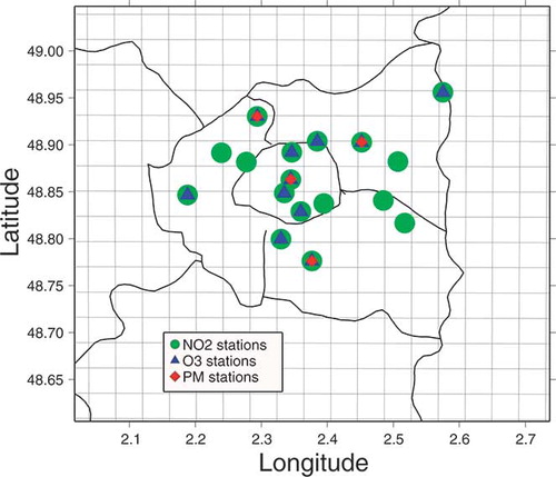
•	CHIMERE surrogate: Area-averaged pollutant concentrations predicted with the CHIMERE air quality model over the epidemiology study domain (counties 75, 92, 93, and 94 as shown in Figure 1a). This is a mean concentration value calculated over downtown and suburban grid cells (3 × 3 CHIMERE cells also shown in Figure 10). This exposure indicator is based on the same assumption of homogeneous exposure as the MONITOR surrogate (area-averaged concentration) with the difference being that concentrations are predicted with the air quality model instead of being measured. Adding this intermediate step in the model evaluation chain is necessary to show the effect of replacing monitor data with air quality model predictions on the results of the epidemiological model.
•	CHIMERE/POP surrogate: Population-weighted modeled concentrations. Here, the information on the population density is included by multiplying predicted concentrations with population fractions for each of the four counties of the epidemiology study domain. This surrogate represents an intermediate case between the simple use of concentration data (MONITOR and CHIMERE surrogates) and the full version also accounting for pollutant concentration spatial variability, demographic, and activity data. The interest of this model evaluation step is to rule out the possibility of increased bias in exposure estimates because of rough modeling assumptions in the construction of the activity diaries.
•	CHIMERE/POP/ACT surrogate: For the calculation of this exposure surrogate, the information on population activity (commuting from home to work) is added. To exclude the rural population from the total 3-Gauss summation model (eq 2) and thus be able to compare model results with the MONITOR model, only the downtown and suburban population fractions of each mode are kept. Modified RWCs (f′i) are calculated for each pollutant, respecting the composition of each mode's population as quantified in the Parameterization section (Figure 8). To include higher order moments of the trimodal distribution (e.g., variance), the 1-Gauss distribution model given by ref 34 is extended for the 3-Gauss summation model applied in the study presented here:

(4)

where μ_i, σ_i, and f′_i represent the mean, variance, and RWC of the ith mode, respectively.

Comparison between Model- and Monitor-Based Surrogates of Exposure

Because the study rests on the ability of the air quality model to predict a population's exposure to outdoor pollutant concentrations, the ability of the CHIMERE model to predict the concentrations measured at the same monitors that have been used to construct the MONITOR exposure surrogates (Figure 10) during the study period is evaluated here. No additional assumptions on the population density or activity patterns have been made here, and only concentration data are being compared. The results are presented in Table 2. The same error metrics to validate the air quality model over the study period are used as in previous studies dedicated to the CHIMERE model validation.35,36 Model scores for all five error metrics are very similar to these studies, showing that the CHIMERE model is able to capture the spatial and temporal variability of pollutant concentration levels with no evidence of systematic biases. Because the exposure surrogates created from the CHIMERE model predictions will be used in a time-series analysis of the atmospheric pollutants' health effects, the authors are interested most of all in the model's ability to capture daily variations in pollutant concentrations. The strongest correlation is found for O₃ (0.83) and the lowest for PM_2.5 (0.54). However, one should keep in mind that model validation forPM_2.5 is based on a small number of monitors inside of the modeling domain (varying from 1 to 4 during the period of the study). With such a low number of MONITOR data, the spatial variability of PM_2.5 concentration cannot be addressed. Therefore, it impossible to judge whether the model is capable of capturing the spatial variability of PM_2.5 over the study domain. This marks the MONITOR and CHIMERE surrogates with a relatively high uncertainty for their ability to correctly assign population exposure.

Table 2. Comparisons between CHIMERE model predictions of O₃ (summer), NO₂, and PM_2.5 concentrations and monitor data

	O3 (summer)	NO2	PM2.5
Mean monitor data (μg/m^3)	81.1	42.5	14.4
Correlation	0.83	0.71	0.54
Bias (μg/m^3)	5.1	0.88	0.97
Normalized bias	8.6%	2.1%	6.8%
RMSE (μg/m^3)	17.7	10.6	7.8
Normalized RMSE	30.1%	25.0%	54.2%
Notes: RMSE = root mean square error.

The next step is to study how the addition of demographic and activity data modifies the time series of the exposure surrogate. Table 3 shows a comparison between MONITOR and CHIMERE/POP/ACT surrogates. For all three pollutants, MONITOR surrogates are higher than the CHIMERE/POP/ACT surrogates by 30, 22 and 29% for NO₂, PM_2.5, and O₃, respectively (mean values). Having ruled out air quality model error as possible source of discrepancy leaves the addition of activity data in the computation of the CHIMERE/POP/ACT exposure surrogates as the only explanation of observed differences. The mean and the median values are close in all cases, which suggests that the values are symmetrically distributed. Comparing the low and high percentiles of NO₂ exposure distributions between the MONITOR and CHIMERE/POP/ ACT surrogates, similar differences are found at low and high values (25th and 75th percentiles). For PM_2.5, the differences between the two models are more marked at low values (25th percentile), whereas for O₃ they are higher at high values (75th percentile)—probably because of an overestimation of O₃ titration by the CTM.

Table 3. Distributions of the monitor- and model-based exposure surrogates for NO₂, PM_2.5, and O₃ (μg/m³) during the study period (2001–2004) at the downtown and suburban areas of the study domain

	NO2				PM2.5				O3 (summer)
	Mean	P25	P50	P75	Mean	P25	P50	P75	Mean	P25	P50	P75
Monitor (μg/m^3)	42.5	32.5	41.7	50.4	14.4	9.8	13.0	17.40	81.1	64.4	77.7	93.7
Model (μg/m^3)	30.80	23.5	30.3	37.0	11.95	7.1	9.9	14.4	57.5	48.8	57.8	66.4
Notes: P25 = 25th percentile, P50 = median, P75 = 75th percentile.

A general remark here is that by taking into account the spatial variability of pollutant concentrations (air quality model instead of monitor data), demographic information (population density), and activity data (travel between work and home) an exposure surrogate was constructed that is more relevant than the MONITOR surrogate, which considers homogeneous exposure for the whole population. Therefore, by using the CHIMERE/ POP/ACT surrogate in the epidemiologic model instead of the MONITOR surrogate, exposure misclassification is expected to decrease, yielding more reliable health risks through the epidemiology application. Even if the resolution of demographic data used for the study presented here was rather low and the activity data were based on rough assumptions, the method should still yield improved health risk estimates compared with a study based on the assumption of homogeneous exposure.

Comparison between Exposure-Response Functions Evaluated by the Different Epidemiological Models

In this part of the analysis, the different exposure surrogates are used in a Poisson regression model on mortality data and the estimated regression coefficients (log relative risks of mortality) yielded by each application are compared to discuss the benefit of having added information on the spatial variability of pollutant concentration within the study domain as well as demographic and activity data. Table 4 shows the coefficients estimated from the regression of the four different surrogates on mortality data. These coefficients are expressed as percent excess in mortality risk associated with a 10-μg/m³ increase in the level of the corresponding exposure surrogate (excess relative risk [ERR]). One different regression is applied for each surrogate type and for each pollutant. The first step is to compare the results between the MONITOR and the CHIMERE surrogates. The ERRs yielded from the MONITOR surrogate (reference studies) show a 1.2, 1.4, and 0.6% increase in mortality because of a 10-μg/m³ increase in PM_2.5, NO₂, and O₃ (only summer period) exposure, respectively. When the CHIMERE surrogate is used for the regression instead of monitor data, all three ERRs are lower (0.9, 1.1, and 0.4%, respectively) and have larger uncertainties. However, the differences are small and may be attributed to the fact that for the construction of the MONITOR surrogates certain already-tested selection criteria were used on the data that could not be applied on the air quality model predictions because this is a new method. The relatively wider confidence intervals (CIs) related to the regression coefficients estimated for PM_2.5 reflect the higher uncertainty in the monitor data and air quality model predictions for this pollutant compared with NO₂ and O₃ concentrations. When predicted concentrations are weighted with population fractions (CHIMERE/POP case), almost no difference is observed in the ERRs compared with the simple CHIMERE case (only the O₃ ERR increases from 0.4 to 0.5%); however, the CIs are now tighter. This shows that even with the rough assumption made here, accounting for activity data in the computation of surrogates adds realism in the representation of exposure. When the complete 3-Gauss summation model is used for the regression on mortality data (CHIMERE/POP/ACT case), a significant decrease is observed in the ERR estimated for NO₂ (decrease from 1.1 to 0.3%), whereas the risks for the other two pollutants are practically unchanged. It should be noted here that no laboratory experiment or cohort study has put in evidence any toxic effect related to NO₂ exposure to date.37,38 The reason why previous epidemiology research such as the reference studies used here (PSAS and APHEA) find positive associations between NO₂ time series and health outcomes is more likely because NO₂ is a good surrogate of traffic emissions, well correlated with ultrafine particles in particular. The positive regression coefficients found for NO₂ thus indirectly reflect the correlation between mortality and traffic rather than to NO₂ itself.39

Table 4. Log relative rates of mortality (ERR) and 95% CIs associated with a 10-μg/m³ increase in the air pollution exposure surrogate

Monopollutant	PM2.5		NO2		O3 ^a
	ERR	95% CI	ERR	95% CI	ERR	95% CI
MONITOR	1.2	[0.2; 2.2]	1.4	[0.9; 1.9]	0.6	[0.1; 1.0]
CHIMERE	0.9	[−0.5; 2.3]	1.1	[0.0; 2.3]	0.4	[0.0; 0.9]
CHIMERE/POP	0.9	[−0.5; 2.3]	1.1	[0.1; 2.1]	0.5	[0.0; 1.0]
CHIMERE/POP/ACT	0.9	[−0.2; 2.0]	0.3	[−0.4; 1.0]	0.4	[−0.4; 1.2]
Notes: PM2.5, NO2, and O3 exposure surrogates are separately introduced to the log-linear regression model (monopollutant model). ^aOnly summer period effects are shown for O3.

The problem of differentiating the health effects among co-pollutants becomes much clearer when treating all three pollutants as covariates is attempted in the same regression (Table 5). Here, the same four different surrogates of exposure for each pollutant are used, but one single regression per surrogate type is applied. All three pollutants are simultaneously injected into the model as covariates, and the ERRs estimated for each one of the pollutants can be compared one with the other in this case. This is a much more realistic representation of the way air pollution affects human health considering that in nature pollutants are inhaled as complex mixtures and not one at a time. As shown in Table 5, the MONITOR surrogate is incapable of differentiating the effects of copollutants: Negative exposure-response functions are estimated for PM_2.5, and the ERR for NO₂ is increased from 1.4 to 1.9% to overcome this negative effect. This is because of the strong correlation between NO₂ and PM_2.5(0.73). It has been shown that in presence of strong correlations among co-pollutants, the regression will converge to coefficients that overestimate the association between the health outcome and the pollutant that is “better” measured even if another correlated co-pollutant is more hazardous.40 For example, in the case of the PSAS and APHEA projects, PM_2.5 is measured at only one to four sites over the study area, whereas 15 and 12 measurement sites are available for NO₂ and O₃, respectively.Because of the larger spatial monitoring coverage of NO₂ over the study domain compared with PM_2.5, the latterabsorbs all of the effect that should be (theoretically) attributed to PM_2.5. The CHIMERE and CHIMERE/POP surrogates suffer from the same effect: The PM_2.5 ERRsdecrease from 0.9% to 0.2 and 0.3%, respectively, whereas NO₂ and O₃ ERRs increase to compensate for the effect (ERRs for O₃ increase from 0.4 and 0.5%, respectively, to1.6%). On the contrary, the problem is not present in the regression of the CHIMERE/POP/ACT surrogate on mortality data: ERRs for PM_2.5 and O₃ are similar to the those estimated in the MONITOR case for the monopollutant regression and the ERR for NO₂ is similar to the one estimated with the CHIMERE/POP/ACT surrogate (within tighter CIs) also in the monopollutant regression (Table 4). In the case of the MONITOR surrogate, only NO₂ comes out with statistically significant t scores, and in the case of the CHIMERE and CHIMERE/POP surrogates, only the O₃ estimate is statistically significant.

Table 5. Log relative rates of mortality (ERR) and 95% CIs associated with a 10-μg/m³ increase in the air pollution exposure surrogate

Three Pollutants	PM2.5		NO2		O3 ^a
	ERR	95% CI	ERR	ERR	95% CI	ERR
MONITOR	−1.1	[−2.6; 0.5]	1.9	[1.1; 2.7]	0.4	[0.0; 0.9]
CHIMERE	0.2	[−0.5; 1.0]	1.4	[−0.3; 3.1]	1.6	[0.1; 3.1]
CHIMERE/POP	0.3	[−0.6; 1.2]	1.4	[−0.5; 3.4]	1.6	[0.1; 3.1]
CHIMERE/POP/ACT	1.3	[−0.0; 2.7]	0.4	[−0.6; 1.4]	0.9	[−0.4; 1.2]
Notes: PM2.5, NO2, and O3 exposure surrogates are simultaneously introduced to the log-linear regression model (three-pollutant model). ^aOnly summer periods effects are shown for O3.

Thus, it appears that the CHIMERE/POP/ACT surrogate provides the opportunity to distinguish among the relative effects of the three pollutants in a multipollutant regression setting. Indeed, when population activity patterns are taken into account in building the exposure surrogate, the time series of co-pollutants are less correlated one with the other. The strong correlation among co-pollutants mostly affects the risk estimates for PM_2.5. The reason for this is that this pollutant is marked with the highest uncertainty. Table 6 shows correlation coefficients between PM_2.5 and the other two co-pollutants (NO₂ and O₃) for each one of the four types of exposure surrogates. A significant decrease in the correlation between PM_2.5 and the other two co-pollutants is found for the CHIMERE/POP/ACT surrogate compared with the CHIMERE and CHIMERE/POP cases: Correlation between PM_2.5 and NO₂ decreases from 0.76 to 0.6 and for PM_2.5 and O₃ from approximately 0.42 to 0.37. This explains why it has been possible to differentiate the effects among the three co-pollutants by using this exposure metric.

Table 6. Correlation between the time series of co-pollutants estimated for four different types of exposure surrogates

	PM2.5 vs. NO2	PM2.5 vs. O3
MONITOR	0.73	−0.15
CHIMERE	0.76	−0.43
CHIMERE/POP	0.76	−0.41
CHIMERE/POP/ACT	0.60	−0.37

CONCLUSIONS

The benefit of using air quality model predictions combined with time-activity data as exposure surrogates instead of central monitors was evaluated in an epidemio-logical study. Although the framework relies on rough assumptions, especially related to the definition of time activity, it was still possible to yield insight into how pollutant-specific health effects may be evidenced following the approach presented here, whereas they were masked by the high correlation among co-pollutants in the more traditional monitor-based approach.

Four-year concentrations of O₃, NO₂, and PM_2.5 were modeled with the CHIMERE CTM over the greater Paris region. Concentration predictions were combined with county-level census data through a Monte Carlo simulation, and a three-activity diary was created for a sample population in the greater Paris region. Three discrete modes were identified in the distribution of exposures among the population, highlighting the heterogeneity of exposure at the regional scale. To quantify the geographical composition of the population of the three exposure modes, a parametrization was developed based on a 3-Gauss summation model. Each exposure mode was further mapped to the downtown, suburban, and rural populations of the Paris region.

To study the value of the developed methodology from an air pollution health effect endpoint, the derived parametrization was used to compute surrogates of exposure for an epidemiological model developed for a previous study on the short-term associations between air pollution and mortality. It was first shown that the use of air quality model predictions instead of monitor data does not dramatically increase the overall bias of the health risk estimation. When pollutant concentration fields are further combined with activity data, the uncertainty in the risk estimates decreases, showing that exposure predictions remain realistic even if rough assumptions were made for the definition of activity data. The principal outcome of the model evaluation in the epidemiological framework was that because of the possibility of accounting for many atmospheric contaminants in a spatially resolved way, the correlation among the exposure surrogates of different co-pollutants was decreased, therefore unmasking pollutant-specific effects.

Depending on the pollutant (presence of indoor sources or not) and the type of exposure (in-vehicle, air conditioning, etc.) distinction between outdoor and indoor exposure is bound to alter model results. NO_x and particulate matter on-road concentration levels modeled here with the subgrid-scale implementation are presumably good surrogates of in-vehicle exposures.41 For O₃, titration by NO leads to a decrease in indoor concentration levels and further adjustments should be implemented in the model to more accurately assign exposure. Another aspect not accounted for is the variability in commute modes that is also bound to affect exposure burden.42 These shortcomings need to be addressed for further applications of the parametrization developed here.

REFERENCES

- Pope , C.A. and Dockery , D.W. 2006 . Health Effects of Fine Particulate Air Pollution: Lines that Connect . Journal of the Air & Waste Management Association , 56 : 709 – 742 .
- Levy , J.I. , Chemerynski , S.M. and Sarnat , J.A. 2005 . Ozone Exposure and Mortality: An Empiric Bayes Metaregression Analysis . Epidemiology , 16 : 458 – 468 .
- Dominici , F. , Peng , R.D. , Bell , M.L. , Pham , L. , McDermott , A. , Zeger , S.L. and Samet , J.M. 2006 . Fine Particulate Air Pollution and Hospital Admission for Cardiovascular and Respiratory Diseases . JAMA , 295 : 1127 – 1134 .
- Cohen , A.J. , Ross Anderson , H. , Ostro , B. , Pandey , K.D. , Krzyzanowski , M. , Kunzli , N. , Gutschmidt , K. , Pope , A. , Romieu , I. , Samet , J.M. and Smith , K. 2005 . The Global Burden of Disease Due to Outdoor Air Pollution . J. Toxicol. Environ. Health Part A. , 68 : 1301 – 1307 .
- Schwartz , J. 1999 . Air Pollution and Hospital Admissions for Heart Disease in Eight U.S. Counties . Epidemiology , 10 : 17 – 22 .
- Anderson, R.; Atkinson, R.; Peacock, J.; Marston, L.; Konstantinou, K. Meta-Analysis of Time-Series Studies and Panel Studies of Particulate Matter (PM) and Ozone (O3); World Health Organization http://www.euro.who.int/_data/assets/pdf_file/0004/74731/e82792.pdf (http://www.euro.who.int/_data/assets/pdf_file/0004/74731/e82792.pdf) (Accessed: 2010 ).
- Bell , M.L. , Dominici , F. and Samet , J.M. 2005 . A Meta-Analysis of Time-Series Studies of Ozone and Mortality with Comparison to the National Morbidity, Mortality, and Air Pollution Study . Epidemiology , 16 : 436 – 445 .
- Sarnat , J.A. , Wilson , W.E. , Strand , M. , Brook , J. , Wyzga , R. and Lumley , T. 2007 . Panel Discussion Review: Session 1—Exposure Assessment and Related Errors in Air Pollution Epidemiologic Studies . J. Expo. Sci. Environ. Epidemiol. , 17 ( Suppl 2 ) : S75 – S82 .
- Traffic-Related Air Pollution: A Critical Review of the Literature on Emissions, Exposure, and Health Effects; Health Effects Institute: Cambridge, MA, 2010 http://pubs.healtheffects.org/view.php?id=334 (http://pubs.healtheffects.org/view.php?id=334) (Accessed: 2010 ).
- Zeka , A. and Schwartz , J. 2004 . Estimating the Independent Effects of Multiple Pollutants in the Presence of Measurement Error: An Application of a Measurement-Error-Resistant Technique . Environ. Health Perspect. , 112 : 1686 – 1690 .
- Kelsall , J.E. , Samet , J.M. , Zeger , S.L. and Xu , J. 1997 . Air Pollution and Mortality in Philadelphia, 1974–1988 . Am. J. Epidemiol. , 146 : 750 – 762 .
- Sarnat , J.A. , Brown , K.W. , Schwartz , J. , Coull , B.A. and Koutrakis , P. 2005 . Ambient Gas Concentrations and Personal Particulate Matter Exposures: Implications for Studying the Health Effects of Particles . Epidemiology , 16 : 385 – 395 .
- Carrothers , T.J. and Evans , J.S. 2000 . Assessing the Impact of Differential Measurement Error on Estimates of Fine Particle Mortality . Journal of the Air & Waste Management Association , 50 : 65 – 74 .
- Kim , J.Y. , Burnett , R.T. and Neas , L. 2007 . Panel Discussion Review: Session Two—Interpretation of Observed Associations between Multiple Ambient Air Pollutants and Health Effects in Epidemiologic Analyses . J. Expo. Sci. Environ. Epidemiol. , 17 ( Suppl 2 ) : S83 – S89 .
- Glen , G. 2002 . User's Guide for the APEX3 Models , Fairfax , VA : ManTech Environmental Technology .
- Rosenbaum , A. 2002 . The HAPEM’4 User's Guide Hazardous Air Pollutant Exposure Model, Version 4 , Research Triangle Park , NC : U.S. Environmental Protection Agency; Office of Air Quality Planning and Standards .
- Burke , J.M. , Zufall , M.J. and Ozkaynak , H. 2001 . A Population Exposure Model for Particulate Matter: Case Study Results for PM2.5 in Philadelphia, PA . J. Expo. Anal. Environ. Epidemiol. , 11 : 470 – 489 .
- Valari , M. and Menut , L. 2010 . Transferring the Heterogeneity of Surface Emissions to Variability in Pollutant Concentrations over Urban Areas through a Chemistry-Transport Model . Atmos. Environ. , 44 : 3229 – 3238 .
- 2008 . “ Air and Health Monitoring Program-9 cities ” . In Monitoring the Health Effects of Air Pollution at Urban environment-Phase II , Saint Maurice: InVS .
- Touloumi , G. , Atkinson , R. , Tertre , A.L. , Samoli , E. , Schwartz , J. , Schindler , C. , Vonk , J.M. , Rossi , G. , Saez , M. , Rabszenko , D. and Katsouyanni , K. 2004 . Analysis of Health Outcome Time Series Data in Epidemiological Studies . Environmetrics , 15 : 101 – 117 .
- Vautard , R. , Beekmann , M. , Roux , J. and Gombert , D. 2001 . Validation of a Hybrid Forecasting System for the Ozone Concentrations over the Paris Area; Atmos. Environ , 35 : 2449 – 2461 .
- Vautard , R. , Menut , L. , Beekmann , M. , Chazette , P. , Flamant , P.H. , Gombert , D. , Guédalia , D. , Kley , D. , Lefebvre , M.P. , Martin , D. , Mégie , G. , Perros , P. and Toupance , G. 2003 . A Synthesis of the Air Pollution over the Paris Region (ESQUIF) Field Campaign . J. Geophys. Res. , 108 doi: 10.1029/2003JD003380
- Ginoux , P. , Chin , M. , Tegen , I. , Prospero , J.M. , Holben , B. , Dubovik , O. and Lin , S.-H. 2001 . Sources and Distributions of Dust Aerosols Simulated with the GOCART Model . J. Geophys. Res. , 106 : 20255 – 20273 .
- van Leer , B. 1979 . Towards the Ultimate Conservative Difference Scheme. V—a Second-Order Sequel to Godunov's Methods . J.Computat. Phys. , 32 : 101 – 136 .
- Tiedtke , M. 1989 . A Comprehensive Mass Flux Scheme for Cumulus Parameterization in Large-Scale Models . Mon. Wea. Rev. , 117 : 1779 – 1800 .
- Hauglustaine , D.A. , Hourdin , F. , Jourdain , L. , Filiberti , M.-A. , Walters , S. , Lamarque , J.-F. and Holland , E.A. 2004 . Interactive Chemistry in the Laboratoire de Météorologie Dynamique General Circulation Model: Description and Background Tropospheric Chemistry Evaluation . J. Geophys. Res. , 109 : D04314 doi: 10.1029/2003JD003957
- Hong , S. , Noh , Y. and Dudhia , J. 2006 . A New Vertical Diffusion Package with an Explicit Treatment of Entrainment Processes . Mon. Wea. Rev. , 134 : 2318 – 2341 .
- Chen , F. and Dudhia , J. 2001 . Coupling an Advanced Land Surface-Hydrology Model with the Penn State–NCAR MM5 Modeling System. Part I: Model Implementation and Sensitivity . Mon. Wea. Rev. , 129 : 569 – 585 .
- Touma , J.S. , Isakov , V. , Ching , J. and Seigneur , C. 2006 . Air Quality Modeling of Hazardous Pollutants: Current Status and Future Directions . J. Air & Waste. Manage. Assoc. , 56 : 547 – 558 .
- Isakov , V. , Irwin , J.S. and Ching , J. 2007 . Using CMAQ for Exposure Modeling and Characterizing the Subgrid Variability for Exposure Estimates . J. Appl. Meteorol. Climatol. , 46 : 1354 – 1371 .
- Ott , W.R. 1990 . A Physical Explanation of the Lognormality of Pollutant Concentrations . Journal of the Air & Waste Management Association , 40 : 1378 – 1383 .
- Shaddick , G. , Zidek , L. and Salway , R. 2008 . Estimating Exposure Response Functions Using Ambient Pollution Concentrations . Ann. Appl. Stat. , 2 : 1249 – 1270 .
- Dominici , F. , McDermott , A. , Zeger , S.L. and Samet , J.M. 2002 . On the Use of Generalized Additive Models in Time-Series Studies of Air Pollution and Health . Am. J. Epidemiol. , 156 : 193 – 203 .
- Richardson , S. , Stucker , I. and Hemon , D. 1987 . Comparison of Relative Risks Obtained in Ecological and Individual Studies: Some Methodological Considerations . Int. J. Epidemiol. , 16 : 111 – 120 .
- Rouil , L. , Honoré , C. , Vautard , R. , Beekmann , M. , Bessagnet , B. , Malherbe , L. , Meleux , F. , Dufour , A. , Elichegaray , C. , Flaud , J.-M. , Menut , L. , Martin , D. , Peuch , A. , Peuch , V.-H. and Poisson , N. 2009 . Prev'Air: An Operational Forecasting and Mapping System for Air Quality in Europe . Bull. Am. Meteorol. Soc. , 90 : 73 – 83 .
- Honoré , C. , Rouïl , L. , Vautard , R. , Beekmann , M. , Bessagnet , B. , Du-four , A. , Elichegaray , C. , Flaud , J.-M. , Malherbe , L. , Meleux , F. , Menut , L. , Martin , D. , Peuch , A. , Peuch , V.-H. and Poisson , N. 2008 . Predictability of European Air Quality: Assessment of 3 Years of Operational Forecasts and Analyses by the PREV'AIR System . J. Geophys. Res. , 113 : D04301 doi: 10.1029/2007JD008761
- Pope , C.A. 2000 . Epidemiology of Fine Particulate Air Pollution and Human Health: Biologic Mechanisms and Who's at Risk . Environ. Health Perspect. , 108 ( Suppl 4 ) : 713 – 723 .
- Favier , A. 2003 . Oxidative Stress: Interest in Experimental and Conceptual Understanding of Disease Mechanisms and Therapeutic Potential (in French) . L'Actualité Chimique. , 269 : 108 – 115 .
- Brook , J.R. , Burnett , R.T. , Dann , T.F. , Cakmak , S. , Goldberg , M.S. , Fan , X. and Wheeler , A.J. 2007 . Further Interpretation of the Acute Effect of Nitrogen Dioxide Observed in Canadian Time-Series Studies . J. Expo. Sci. Environ. Epidemiol. , 17 ( Suppl 2 ) : S36 – S44 .
- Dominici , F. , Zeger , S.L. and Samet , J.M. 2000 . A Measurement Error Model for Time-Series Studies of Air Pollution and Mortality . Biostat. , 1 : 157 – 175 .
- Fruin , S. , Westerdahl , D. , Sax , T. , Sioutas , C. and Fine , P. 2008 . Measurements and Predictors of On-Road Ultrafine Particle Concentrations and Associated Pollutants in Los Angeles . Atmos. Environ. , 42 : 207 – 219 .
- Tsai , D. , Wu , Y. and Chan , C. 2008 . Comparisons of Commuter's Exposure to Particulate Matters while Using Different Transportation Modes . Sci. Total Environ. , 405 : 71 – 77 .