Issues with Ozone Attainment Methodology for Houston, TX

ABSTRACT

To comply with the federal 8-hr ozone standard, the state of Texas is creating a plan for Houston that strictly follows the U.S. Environmental Protection Agency's (EPA) guidance for demonstrating attainment. EPA's attainment guidance methodology has several key assumptions that are demonstrated to not be completely appropriate for the unique observed ozone conditions found in Houston. Houston's ozone violations at monitoring sites are realized as gradual hour-to-hour increases in ozone concentrations, or by large hourly ozone increases that exceed up to 100 parts per billion/hr. Given the time profiles at the violating monitors and those of nearby monitors, these large increases appear to be associated with small parcels of spatially limited plumes of high ozone in a lower background of urban ozone. Some of these high ozone parcels and plumes have been linked to a combination of unique wind conditions and episodic hydrocarbon emission events from the Houston Ship Channel. However, the regulatory air quality model (AQM) does not predict these sharp ozone gradients. Instead, the AQM predicts gradual hourly increases with broad regions of high ozone covering the entire Houston urban core. The AQM model performance can be partly attributed to EPA attainment guidance that prescribes the removal in the baseline model simulation of any episodic hydrocarbon emissions, thereby potentially removing any nontypical causes of ozone exceedances. This paper shows that attainment of all monitors is achieved when days with observed large hourly variability in ozone concentrations are filtered from attainment metrics. Thus, the modeling and observational data support a second unique cause for how ozone is formed in Houston, and the current EPA methodology addresses only one of these two causes.

IMPLICATIONS

Observational analysis in Houston provides compelling evidence that ozone design values at some surface monitors are dominantly influenced by large hourly changes in ozone concentration that are not predicted by the regulatory model. The use of these models, with current EPA attainment methodology, produces policies that likely overestimate precursor control requirements because only one cause of ozone is functioning in the model. This issue has significant regulatory and economic implications for Houston, especially under lower National Ambient Air Quality Standards. An attainment methodology that recognizes two unique causes for high ozone potentially offers a more reliable means for developing and justifying control policies.

View correction statement:

Erratum

INTRODUCTION

Several factors combine to make Houston's ozone (O₃) problem unique in comparison to other metropolitan cities in the United States. These include the (1) complex interactions between land-sea breeze circulations, (2) intense clustering of industrial emission sources in the Houston Ship Channel and coastal areas, (3) significant precursor emissions from the heavily urbanized eight-county Houston Galveston Bay (HGB) area, and (4) potential pollution transport from domestic and international source regions. The culmination of these factors has resulted in a complex and difficult environment to understand. This difficulty has garnered the attention of researchers and regulators with the common goal of understanding how O₃ is formed. The resulting science and policies of Texas regulators describe two unique causes, or conceptual models, for how high O₃ is formed in Houston. One conceptual model is a gradual region-wide increase in O₃ concentrations “typical” of many large U.S. metropolitan cities. This conceptual model is well represented in the gradual evolution of O₃ seen in observations and predicted in photochemical models. The second conceptual model was first discovered in Houston and has been linked to episodic emission events of volatile organic compounds (VOCs). On days with unique wind conditions,1,1a these emissions produce narrow plumes of high O₃ concentrations that appear in only a few surface measurements as large changes in hourly O₃ concentrations, or nontypical ozone changes (NTOCs). On the basis of this dual conceptual model for high O₃, the Texas Commission on Environmental Quality (TCEQ) proposed, and the U.S. Environmental Protection Agency (EPA) accepted, a dual mitigation approach in their 2004 State Implementation Plan (SIP) aimed at showing attainment of the 1-hr federal O₃ standard.1b,2

The 2004 SIP established for the first time a dual-O₃ management paradigm in Houston, TX. In this SIP, TCEQ recognized that relatively small amounts of short-term emissions from particular industrial sources of highly reactive alkenes could lead to large short-duration peak O₃ that then skewed the design values for 1-hr O₃. Most of these highest observations occurred at only a single monitor for a day. Using observational and modeling evidence, the TCEQ proposed an innovative method that targeted four VOCs termed “highly reactive VOCs” (HRVOCs), which include ethene, propene, 1,3-butadiene, and all butenes.1b,2 Management strategies were developed to reduce the short-term and highly variable industrial releases of HRVOCs. A maximum not-to-exceed hourly rate of 1200 lb/hr was proposed by the TCEQ and was subsequently formally adopted by EPA. As defined in TCEQ's 2004 mid-course SIP, this short-term cap applied to unauthorized emissions and permitted emissions that may fluctuate on an hourly basis. Compliance with these new HRVOC controls necessitated significant abatement investments by certain industrial sources. Indeed, polymer production facilities in the region were reported to have spent up to $2.4 million in equipment to monitor and reduce HRVOCs.3

In addition to these innovative policy strategies, the TCEQ and selected industries have also used infrared (IR) camera technology for pollution detection.4 This technology allows emitters and regulators to view emission plumes that are not visible to the naked eye. In 2005, the camera helped to identify more than 7000 t/yr of VOC emissions that were then eliminated.5 Responding to this increased regulatory emphasis on HRVOC emissions, several Houston industrial facilities also purchased cameras and now use them as part of their leak detection programs. As a result of the increased use of the IR cameras and HRVOC regulations, the TCEQ has reported significant reductions in annual averaged measured concentrations of these species at several monitoring sites.6,7 Since the approval of the 2004 SIP and adoption of its policies, there have been significant reductions in measured peak O₃ at several monitors across Houston. The success of this SIP is grounded in the recognition of the dual O₃ problem in Houston.

The state of Texas is now grappling with how it will show attainment of the 1997 8-hr O₃ standard of 0.08 parts per million (ppm). This new O₃ metric and an updated national attainment methodology have been applied for the first time in Houston by the TCEQ for their 2010 SIP. For the new SIP, the TCEQ has developed the observational and modeling database needed to complete the prescribed EPA attainment demonstration. Given the SIP deadline and the planning of a new observational field program in 2006, the TCEQ picked episodes in 2005 and 2006 as the basis of the 2010 SIP. In hindsight, it is clear that the conditions present in the modeling periods occurred before the full implementation of the rules promulgated in the 2004 SIP. This study uses the TCEQ's modeling episodes to investigate how Houston's dual O₃ cause is represented in the final 2010 attainment demonstration.

2010 Houston SIP

On March 10, 2010, the TCEQ adopted an 8-hr O₃ SIP aimed at meeting the 1997 8-hr O₃ standard (0.08 ppm).8 The Pennsylvania State University/National Center for Atmospheric Research Fifth-Generation Mesoscale Model (MM5)/Comprehensive Air Quality Model with extensions (CAMx) modeling system,9 supported by the Second Texas Air Quality Study (TexAQS II)10 database, formed the technical foundation of the 2010 SIP. This SIP is the first application in Texas of the new 8-hr O₃ attainment methodology developed by EPA. The EPA, using a national viewpoint, made several defining assumptions in the development of the 8-hr O₃ attainment test methodology. These assumptions stemmed from EPA's recognition of the inherent uncertainty in atmospheric processes and the practical limitations imposed by the computational resources of the mid-1990s. For example, modeling episodes were typically limited to approximately 6- to 8-day episodes. Furthermore, the EPA recognized the need to develop attainment estimates that comported with the 3-yr statistical form of the standard. After deliberations with the scientific review panel, EPA proposed an algebraic attainment test equation that combines selected output from base- and future-year photochemical grid model simulations with measured 8-hr “design values” at individual monitors. This approach is very different from that used in the 2004 SIP that was approved by EPA.

The EPA guidance for attainment demonstration states that the photochemical grid model must use an emission inventory that has only “typical” emissions. This emission inventory will have replaced any dayspecific emissions with average or “typical” emissions for certain types of sources. However, the meteorological input files remained unchanged, retaining their day-specific variability. Implicit in EPA's endorsement of this approach is that daily variability in meteorology, not emissions, is the main driver in causing the highest O₃ concentrations. A second implied assumption is that the fourth-highest O₃ mixing ratios over a 3- to 5-yr period are caused by the same rates of emissions; the possibility of highly variable (in time and space) episodic emissions is not considered. These assumptions were made to create an expedient approach from a national guidance perspective because they greatly simplified the computational and analysis burden faced by states developing O₃ SIPs.

EPA justified the 8-hr attainment test with two unproven assertions. First, incorporating O₃ measurements in the attainment equation “anchored” future projections to actual data, rendering the future projections more reliable. Second, EPA hypothesized that the effects of model uncertainty are reduced when a model is used in a relative, rather than an absolute, sense. The agency further supposed that the resulting error in the relative difference between base and control scenarios should be smaller than the absolute errors. EPA reasoned that the early indications from zero-dimensional chemical kinetic studies on incremental hydrocarbon reactivity11 could be extended to regional scale three-dimensional atmospheric models simulating base and future years often 10 to 15 yr apart. Although never rigorously tested and reported in the science literature, the notion that chemical mechanism sensitivity relationships might hold over major urban areas over times scales of a decade or more never received serious investigation. Many studies have examined the ramifications of the EPA attainment equation12–14 and its sensitivity to model inputs. No one has investigated the implication of applying the attainment equation in a place such as a Houston with its unique causes of O₃ violations. Therefore, the fundamental assumptions and scientific justifications underpinning current regulatory modeling tools and EPA attainment guidance need to be addressed specifically for southeast Texas. In this paper, it is asked whether the EPA attainment method is appropriate for determining the level of precursor controls needed for the unique O₃ problem found in Houston.

METHODOLOGY

EPA O₃ Attainment Methodology

Current EPA O₃ attainment guidance15 was formulated in the late 1990s and was informed by a significant body of previous measurement studies and modeling programs. Dating back to the early 1970s, O₃ formation in major urban areas was understood to result from the mixing and chemical interaction of emissions from several anthropogenic sources common in large metropolitan centers.16–18 Over the course of one to several days, hourly O₃ concentrations undergo a commonly observed diurnal pattern with peak levels attained at different monitors and on different modeled days during the episodes (typically 3–8 days in duration). This traditional paradigm of O₃ cause-and-effect phenomena was imbedded in the formulation of regulatory model and represented in the model inputs, especially the emissions. EPA's guidance for 1-hr O₃ 19 emphasized model usage in a strict deterministic mode; that is, either the standard was passed or not. When the first 8-hr standard was established in 1997, it was expressed in a statistical form (fourth-highest value at a monitor averaged over 3 yr). To facilitate implementation of the new standard, EPA began formulating 8-hr modeling guidance in 1998 supported by an external scientific review panel of approximately 20 experts from across the United States. The first draft of the 8-hr guidance was released in 1999; EPA issued the final guidance in 2007. It is important to note that the guidance is not legally binding and can be altered with approval from EPA.

8-Hr O₃ Attainment Methodology

EPA's attainment equation considers the ratio of grid-model O₃ estimates from future to base levels and observed data from surface monitors. This test is monitor-centric; that is, it is applied separately to each regulatory monitor in nonattainment areas. At each regulatory monitor, the test is passed when the estimated future O₃ metric is lower than the National Ambient Air Quality Standards (NAAQS). In part to account for modeling and data uncertainties, EPA guidance allows for “weight of evidence” analyses to amplify the meaning of the test results.

To determine whether a region is violating the federal standard, an observational-based average called the design value (DV_m) is calculated for every monitor. For a monitor m, a DV_m is calculated as a running 3-yr average of the observed fourth-highest daily peak 8-hr O₃ concentrations, M _(fourth)m. For the year 2006, the method for calculating a DV_m is shown in eq 1.

(1)

where M _(fourth)m is the observed fourth-highest daily peak 8-hr O₃ concentration for monitor m over the O₃ season year.

If the DV_m for a regulatory monitor is equal to or less than the standard, then that monitor is said to be in attainment of the NAAQS. For the region to be declared in attainment, EPA requires that all regulatory monitors have DV_m in compliance with the standard. If the DV_m for any monitor is greater than the standard, then the entire region is considered to have failed to attain the O₃ standard and must follow the EPA guidance for showing attainment.20

All O₃ nonattainment area SIPs must include a demonstration of future attainment. For this purpose, a different observational-based metric is calculated for each monitor—the baseline design value (DV_B,m).20 To calculate a DV_B,m, the policy-maker must first decide on a baseline year. Typically, this year coincides with the year being simulated by the regulatory air quality model. To calculate a DV_B,m, a 5-yr weighted-center method is used as shown in eq 2 for a 2006 baseline year.

(2)

Thus, all DV_B,m values are based on observed monitor values and result in multiyear averaged values of 8-hr averaged values.

The final step of the attainment demonstration is to multiply the DV_B,m by the relative response factor (RRF_m), which is the predicted response to future control strategies of the regulatory AQM. The RRF_m ratio is multiplied by DV_B,m to produce a future design value (DV_F,m) that must be below the federal standard, as shown in eq 3.

(3)

The essence of the attainment test is eq 3. The RRF_m is the algebraic construct EPA proposed to link baseline and future O₃ conditions at individual regulatory monitors. The ramifications and flexibility of EPA's attainment equation have been investigated for nearly a decade,12–14,21,21a and a sizable body of work has been assembled to characterize the spatial variability of the RRF_m values and their sensitivity to the choice of host air quality model. Not long after the first draft modeling guidance was published,15 researchers found that “depending upon the choice of the modeling system, the forecasted DV_m at some monitors could result in them being in attainment or nonattainment.”14 Over the past decade, there has been very little examination of the role that O₃ formation processes have on the RRF_m and its distribution across a dense monitoring network of a major urban center. Most of the focus has been on how different model inputs such as meteorology22 or grid spacing23 affect the RRFs and DV_F,m.

Aerometric Measurements

For this study, we obtained the relevant hourly O₃ measurement data and CAMx model output files (baseline and future) that were used in developing the 2010 Houston O₃ SIP. These data were used by the TCEQ for the modeled attainment demonstration following EPA guidance. DV_B,m and RRF_m values were calculated at 25 ambient monitors throughout the Houston nonattainment area. Twenty of these are regulatory monitors. Table 1 shows that most of these monitors are in attainment or, on the basis of preliminary modeling from the TCEQ, show attainment in the future.24 Observed data were acquired via download from the TCEQ website, which provides hourly averaged measurement data.25 The monitor locations are shown in Figure 1 and are identified with four letters. The monitor's official names, TCEQ identification number, Aerometric Information Retrieval System (AIRS) number, and the four-letter designations used in this work are given in Table 1. Also shown are the calculated DV_B,m and RRF_m for a 2006 baseline year and the 2018 DV_F,m. As shown, there are three monitors with a DV_F,m greater than 85 parts per billion (ppb).

Table 1. Monitor names and their identification used in this study

Monitor Name	Abbreviation	CAMS Number	AIRS Number	DVB,m	RRF	DVF,m
Wallisville	WALV	617	48-201-0617	92.0	0.959	88.2
Deer Park	DRPK	35	48-201-1039	92.0	0.958	88.1
Bayland Park	BAYP	53	48-201-0055	96.7	0.900	87.0
Monroe	HSMA	406	48-201-0062	90.3	0.934	84.3
Manvel Croix Park	MACP	84	48-039-1004	90.7	0.900	81.6
Seabrook Friendship Park	SBFP	45	48-201-1050	85.3	0.946	80.7
HRM-3 Haden Road	H03H	603	48-201-0803	84.0	0.959	80.6
Texas City	TXCT	620	48-167-0056	84.3	0.947	79.8
Westhollow	SHWH	410	48-201-0066	92.3	0.859	79.3
Galveston	GALC	34	48-167-0014	83.0	0.955	79.3
Channelview	HCHV	15	48-201-0026	82.7	0.958	79.2
Lynchburg Ferry	LYNF	1015	48-201-1015	81.7	0.961	78.5
Croquet	HCQA	409	48-201-0051	87.0	0.900	78.3
Aldine	HALC	8	48-201-0024	85.0	0.920	78.2
Mustang Bayou	MSTG	619	48-039-0619	84.7	0.917	77.7
Northwest Harris County	HNWA	26	48-201-0029	89.0	0.869	77.3
Houston East	HOEA	1	48-201-1034	80.3	0.959	77.0
Houston Regional Office	HROC	81	48-201-0070	79.7	0.960	76.5
Clinton	CLIN	403	48-201-1035	79.0	0.959	75.8
Texas Avenue	HTCA	411	48-201-0075	79.3	0.943	74.8
Conroe Relocated	CNR2	78	48-339-0078	83.0	0.877	72.8
Danciger	DNCG	618	48-039-0618	80.3	0.894	71.8
North Wayside	HWAA	405	48-201-0046	76.3	0.937	71.5
Lake Jackson	LKJK	1016	48-039-1016	77.0	0.903	69.5
Lang	HLAA	408	48-201-0047	77.7	0.889	69.1
Notes: Also shown are the calculated 2006 DVB,m in ppb, RRF, and 2018 DVF,m in ppb.

Figure 1. Location of surface monitors near downtown Houston used in the attainment demonstration. The BAYP, DRPK, and WALV monitors have DV_F,m above 85 ppb and are labeled with an asterisk. The monitors HNWA, CNR2, DNCG, LKJK, MSTG, GALC, and TXCT monitors are also used in the attainment demonstration but are located outside of the map shown here.

Photochemical Model Simulations

The TCEQ used the CAMx version 4.5126 model to create 2005 and 2006 baseline conditions and projected 2018 conditions for six modeling episodes that are shown in Supplemental Table 1 (published at http://secure.awma.org/onlinelibrary/samples/10.3155-1047-3289.61.3.238 supplmaterial.pdf). Detailed documentation concerning the development of the inputs for these episodes can be found on the TCEQ website. In total, there are 120 modeling days in the 2005 and 2006 episodes. To support a multispecies model performance assessment, the TCEQ generated a “base case” inventory for the six episodes. This included the development of an hourly special inventory (SI) that was based on reports from 141 facilities in the region for the period of August 15 to September 15, 2006. Much of the SI was developed from data gathered during the TexAQS II 2006 field program.

For the attainment demonstration, the base case emission inventory was modified and a new 2006 baseline and a 2018 emission inventory were constructed consistent with EPA inventory guidance; that is, the emissions files used for the model evaluation were changed to comport with EPA's “typical” emission criteria. This was accomplished by dropping day-specific emissions data and reverting to O₃ season averaged emissions at electric generating units (EGUs) and other sources. For example, hourly tank landing loss emissions were changed to an average of emission rates and diurnal profiles used in the 2006 base case emission inventory. Following EPA inventory guidance, the TCEQ removed any reported emission events that were specific to 2006. This included the removal of the hourly SI. It is important to note that the 2005 and 2006 model simulations used in the RRF_m calculation retained their date-specific meteorology. In addition to being used in the attainment demonstration, the baseline emission inventory was the basis for the 2018 emission inventory. The emission inventory for 2018 includes all existing emissions controls, projected growth of emissions, and proposed emission controls.

An analysis of these three emission inventories (2006 base case, 2006 baseline, and 2018 baseline) revealed a change in the magnitude of emissions of oxides of nitrogen (NO_x) and VOCs as well as allocations among emission sources. For this analysis, emissions were categorized at a broad level for area sources, non-road mobile sources, on-road mobile sources, and point sources. Emissions were also split into finer categories (e.g., point source petrochemical emissions, on-road mobile source emissions from gasoline-fueled engines). Emissions summaries were evaluated for the eight-county HGB area. All emissions estimates excluding the on-road (link) emissions estimates were developed using the datasets supplied by TCEQ. The on-road (link) emissions estimates were generated using the LBASE emissions files supplied by TCEQ on a removable hard drive.

The 2006 base case and baseline emission inventory data were compiled for the eight counties surrounding Houston. Estimates were averaged over the entire episode period and listed by source. Supplemental Table 2 shows the gains and losses for each source category from the 2006 base case emission inventory. Changing from the base case to the baseline emission inventory resulted in several modifications across several sources. Following the EPA guidance, TCEQ removed 50.8 t/day of NO_x from the SI emissions, citing that they are not typical. Interestingly, the TCEQ then added 12 t/day back to petrochemical point sources, resulting in a net decrease of 38.8 t/day. This addition, plus another 57 t/day added to point non-EGU, resulted in a net increase in NO_x emissions of 20 t/day when the baseline emission inventory is used. A similar pattern is seen in VOC emissions. The SI VOC was removed from point sources, resulting in a reduction of 25.8 t/day, and the TCEQ added back 15.7 t/day of VOCs to petrochemical point sources. The TCEQ also added 2.9 t/day to point non-EGU, 3.7 t/day to point landing losses, and 5.4 t/day to unclassified point sources. The sum of these additions roughly equaled the VOC SI emissions that were dropped as being not typical; the net change was a loss of only 1.6 t/day. This number is misleading because there were significant changes in the allocation of emissions among sources and thus differences in temporal and spatial emissions.

Table 2. The 2003 and 2009 O₃ DV_m and the amount of absolute decrease from 2003 to 2009 for 19 surface monitors

Monitoring Station	2003 DVm (ppb)	2009 DVm (ppb)	Absolute Decrease (ppb)	Relative Decrease (%)
HOEA	100	76	24	24.0
HCQA	99	76	23	23.2
CLIN	96	74	22	22.9
HROC	94	72	22	23.4
DRPK	102	81	21	20.6
GALC	86	65	21	24.4
HSMA	90	71	19	21.1
BAYP	102	84	18	17.6
HALC	100	83	17	17.0
HNWA	100	84	16	16.0
HWAA	86	72	14	16.3
HTCA	88	75	13	14.8
HCHV	87	78	9	10.3
SHWH	87	79	8	9.2
CNR2	78	71	7	9.0
SBFP	85	78	7	8.2
MACP	89	84	5	5.6
HLAA	78	75	3	3.8

Using the 2006 baseline emission inventory, TCEQ created a 2018 emission inventory named “cs04.” As shown in Supplemental Table 2, there is a net reduction in NO_x emissions of 213 t/day. The bulk of these changes were due to a 140-t/day reduction in on-road mobile sources. There was also a large 64.4-t/day reduction in point non-EGU and a 30-t/day loss in area nonroad emissions. In the 2018 emission inventory, there were minimal increases in NO_x, with a 7.7-t/day increase in point EGU and a 6.3-t/day increase in ship emissions. A different trend is evident with VOC emissions. Instead of a net loss, there is a net gain of 44.3 t/day of VOC emissions. This gain is almost entirely attributable to the addition of 114.6 t/day of VOCs to petrochemical point sources. This large increase is offset by a 41.6-t/day reduction in on-road emissions and a 27.4-t/day decrease in nonroad emissions.

RESULTS

The EPA guidance recommends an observational metric, the DV_B,m, and a modeling metric, RRF_m, to determine attainment. The following results will first focus on an assessment of both of these metrics when applied to Houston.

DV_B,m Metric

The EPA attainment guidance methodology was applied to every monitor in Houston, modeling and observational metrics were calculated, and their components were analyzed. These values are shown in Table 1. The analysis focused on monitors that showed difficulty in predicting attainment, were representative of the region, and had a long history of measuring O₃. On the basis of these criteria, seven surface monitors across Houston were chosen from the period of 2000 to 2009. The monitors BAYP, DRPK, and WALV were chosen in part because they have DV_F,m that are above 85 ppb. The HSMA monitor was also chosen because it was barely in attainment with a DV_F,m of 84.3 ppb, as shown in Table 1. The TCEQ also found, through preliminary modeling, that more precursor controls would be needed to attain the federal standard at the BAYP, DRPK, and WALV monitors.24 BAYP is located southwest of the Houston urban core, and the WALV monitor is located north of several large petrochemical sources (Figure 1). Three additional monitors with a long history of operation (CLIN, HALC, and HNWA) were added to represent other geographic regions of Houston. As shown in Figure 1, the CLIN monitor is at the western end of the Houston Ship Channel and is near large oil refineries. The HALC and HNWA monitors are north and northwest, respectively, of downtown Houston and are often impacted by the northern transport of pollutants from the ship channel and the urban core.

The four highest 8-hr O₃ days for each year at each monitor were calculated for 2003–2009. These years encompass the window of potential years that might be used by TCEQ in computing a 2006 baseline-year DV_B,m value. The highest 1-hr O₃ concentration during the 8-hr window of the fourth-highest O₃ was also extracted as an indication of potential O₃ produced from HRVOC events. To help understand source-receptor relationships, the 8-hr averaged ground-level wind vector was also calculated.

A visual display of the components of the DV_m is shown in Figure 2 for the CLIN, WALV, BAYP, and DRPK monitors. Figure 2 shows for each set of three consecutive years on the x-axis the fourth-highest 8-hr O₃ at the monitor for each year. The filled circles are the 8-hr concentrations, and the plus symbols are the 1-hr peak O₃ concentrations during the 8-hr window. The colors of the circles and plus symbols are related to the color of the year labeled on the x-axis. The thick, black horizontal bar shows the DV_m, and the magenta line shows the 1997 8-hr O₃ standard level (85 ppb). As shown in eq 2, a DV_B,m is the average of three DV_m resulting from the use of observations over a 5-yr period.

Figure 2. A visual display of the components of the design value (DV) for the (a) CLIN, (b) WALV, (c) BAYP, and (d) DRPK monitors. For each set of three consecutive years on the x-axis, the fourth-highest 8-hr O₃ values at the monitor for each year are shown. The filled circles are the 8-hr concentrations, and the plus symbols are the 1-hr peak O₃ concentrations during the 8-hr window. The colors of the circles and plus symbols are related to the color of the year label on the x-axis. For each circle, the 8-hr averaged ground-level wind vector is also shown. The thick, black horizontal bar shows the DV, and the magenta line shows the 1997 8-hr O₃ standard level (85 ppb).

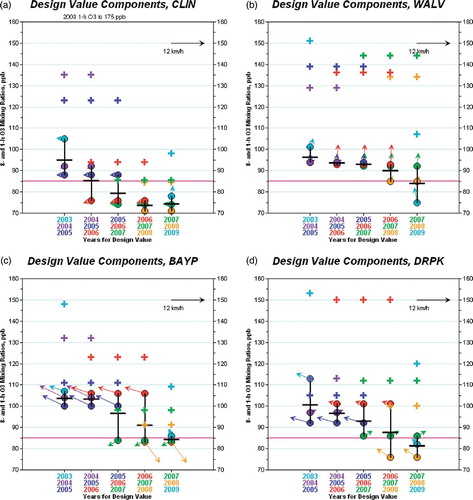
Analysis of these plots for seven monitors revealed that O₃ values have decreased over the 7-yr period. The HNWA, HALC, and HSMA monitors had an observed decrease in 1-hr peak O₃ concentrations that was similar to the CLIN monitor as shown in Figure 2. The other three monitors in Figure 2 also show a decreasing trend but are not as steep, resulting in a 2008 DV_m equal to or greater than 85 ppb. Only in 2009 did these DV_m fall below 85 ppb. This downward trend of DV_m is underscored by the fact that five of the seven monitors show a DV_m decrease each year. One monitor, HSMA, had a DV_m increase once during this period; HNWA had DV_m remain the same for two consecutive years. Of these seven monitors, the CLIN monitor showed the largest decrease, 22 ppb, dropping from 96 ppb in 2003 to 74 ppb in 2009. Table 2 lists the absolute decrease (ppb) in DV_m from 2003 to 2009 for the 19 monitors that had O₃ data. Several monitors near CLIN, specifically HOEA and HROC, also had similar drops in DV_m from 2003 to 2009. As shown in Figure 1, these three monitors are located geographically near each other, suggesting that they could be affected by the same reductions in an upwind emission source. Table 2 shows that every monitor saw a reduction in their DV_m from 2003 to 2009, with differences ranging from 3 to 24 ppb. The largest decreases were seen at the monitors with the highest 2003 DV_m.

Using the data from Figure 2, the ratio between the fourth-highest 8-hr O₃ concentration and the 1-hr peak O₃ concentration during that 8-hr period was calculated. When 1-hr values are high relative to the 8-hr value, it suggests that nontypical, sharp O₃ changes may have contributed to the DV_m. These nontypical, sharp changes have been associated with nonpermitted HRVOC emissions. For example, in Figure 2, the CLIN monitor in 2003 had an 8-hr O₃ concentration of 105 ppb and a 1-hr peak O₃ concentration of 175 ppb. This 2003 value occurred on October 20th, and TCEQ concluded that this was the result of an upwind emission release of a substantial amount of HRVOCs.27 The 2004 and 2005 fourth-highest O₃ concentrations for CLIN were both near 90 ppb and had 1-hr O₃ concentrations of 135 and 123 ppb (ratios of 1.48 and 1.40), respectively. Subsequent years at CLIN show dramatic declines in the peak 1-hr O₃ values with concentrations of 94 and 85 ppb. Clearly there was a significant change at the CLIN monitor over this period.

Figure 2 presents the 8-hr averaged wind vector attached to the year's 8-hr O₃ value and shown originating from the monitor data point. The BAYP and DRPK monitors had 8-hr average vector winds associated with high-DV_m days from different directions, whereas two monitors (CLIN and WALV) showed no variation in wind direction. Constant wind direction for DV_m days, like at CLIN and WALV, means that high observed O₃ at this site had a similar source-receptor relationship across all DV_m days. However, if the pattern changes, then meteorology has changed for that time period or a source that used to be upwind has changed and a new source has become more important. At the WALV monitor, the 2008 DV_m is only 6 ppb less than its 2005 DV_m. This is the smallest observed decrease and is also less than half of the average decrease of the seven monitors.

RRF Metric

The RRF_m is the ratio of average 8-hr maximum O₃ concentrations from the baseline () and future attainment year () simulations.15 Figure 3 shows the baseline (blue) and future-year (green) averages used in the RRF_m calculation for 25 monitors. The monitors are geographically listed along the x-axis from west to east. The six monitors on the far right of the plot are more than 25 km from the Houston urban core and are less likely to be influenced by HRVOC events. Also shown in Figure 3 are the DV_B,m values for each monitor. The DV_B,m for the BAYP, HSMA, DRPK, and WALV monitors are some of the highest in the domain, with 8-hr average concentrations above 90 ppb. Also evident in the plot is the striking difference in DV_B,m concentrations from monitors that are geographically relatively close to each other. For example, the BAYP monitor has a DV_B,m of 96.7 ppb, but only 8 km to the south the HCQA monitor has a DV_B,m of 87 ppb. Likewise, the HLAA monitor, located only 16 km to the north of BAYP, has a DV_B,m concentration of 77.7 ppb. As shown in Figure 1, all three monitors are approximately the same distance from the heavily industrial east side of Houston, and despite close proximity, they exhibit dramatically different DV_B,m concentrations. Analysis of O₃ time series for the top four highest 8-hr O₃ days at each monitor revealed that the BAYP had more days with NTOC characteristics than the other two monitors. These data suggest an upwind source for which the impact is so spatially limited that it frequently impacts a single monitor given the typical wind flow patterns for these years.

Figure 3. For 25 monitors, the baseline (blue) and future-year (green) averages used in the RRF calculation. The monitors are geographically listed along the x-axis from west to east. The six monitors on the far right of the plot are more than 25 km from the Houston urban core and are less likely to be influenced by HRVOC events. Also shown are the DV_B,m values for each monitor. The BAYP, DRPK, and WALV monitors have DV_F,m above 85 ppb, and the HSMA DV_F,m is 84.3 ppb. These four monitors are labeled with an asterisk and are highlighted with a purple arrow.

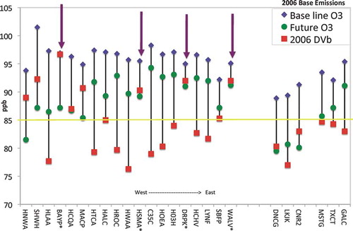
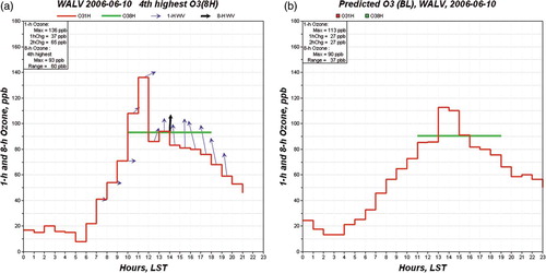
More importantly, the observed spatial heterogeneity seen in the DV_B,m is absent in model predictions. Model predictions used to calculate the baseline modeling average (), as shown in Figure 3, have values that are clustered near 97 ppb with the largest value predicted at the SHWH monitor (102 ppb). Thus, the baseline regulatory model predictions do not replicate the spatial trends seen in the DV_B,m values. There were also significant differences in model-predicted O₃ and observational time series for NTOC days. Figure 4 shows observed values at the WALV monitor on June 10, 2006 and the model-predicted O₃ at that location. It is clear from the figure that the model was unable to match the hourly change in O₃ concentrations or the peak magnitude. At 10:00 a.m. local standard time (LST), the monitor recorded a 1-hr O₃ concentration of 108 ppb, a 37-ppb increase from the 9:00 a.m. measurement of 71 ppb. At 11:00 a.m. LST, the observed O₃ concentration increased to 136 ppb, which is the daily peak for this monitor. The model predicted only 85 ppb at 11:00 a.m., missing the observed peak by 51 ppb. In addition, the model did not simulate the rapid rise in O₃ concentrations in the morning, predicting gradual hourly increases of approximately 10 ppb. There is a second observed peak at 1:00 p.m. LST when there is an observed wind shift. Although the model was able to capture the timing of the peak, the model overpredicted the O₃ concentration by 18 ppb. The combined effect of over- and underpredictions by the model results in the maximum daily 8-hr O₃ concentrations differing by only 3 ppb from the observed value, as indicated by the green line in Figure 4. This type of model performance occurs on several attempts to simulate observed NTOC days. These data suggest that the averaging methodology and modifications to the emission inventory have succeeded in creating model predictions of gradual increases in O₃ concentration without sharp gradients.

Figure 4. O₃ time series plots from (a) observations and (b) model predictions at the WALV monitor. The time series on the left shows the hourly averaged O₃ concentration measurements in red and measured hourly resultant wind vectors in blue. The green line represents the peak 8-hr O₃ concentration, the 8-hr window that was used, and a black arrow shows the 8-hr resultant wind vector. The time series on the right shows the hourly averaged predicted O₃ concentration in red from the TCEQ regulatory model at a 2-km resolution. The green line represents the peak 8-hr O₃ concentration and the 8-hr window that was used.

The second component of the RRF_m is the average of future-year 8-hr maximum O₃ concentrations, or . These values show an interesting spatial trend. At the monitor locations on the western side of Houston, the regulatory model predicted a larger reduction due to precursor reductions than the eastern monitors. The controls proposed in this future emission inventory would be effective if DV_B.m values were higher in the western monitors than the eastern monitors. In fact, several eastern monitors such as WALV, DRPK, and HSMA have some of the highest DV_B,m concentrations. Thus, faced with such a small predicted response at these monitor locations, users of the regulatory model would have to enforce even tighter controls in Houston in an attempt to bring these three monitors into compliance.

NTOC and Attainment Metrics

Houston's O₃ problem is seen in observations as rapid 1-hr concentration increases or more gradual increases that build to values above 85 ppb for a sustained time. Daily maximum 8-hr averages at a monitor may be exceeding the 8-hr NAAQS because of only 1 or 2 hr of very high O₃, which only appears at a spatially limited number of monitors and thus cannot be “typical.” Therefore, understanding the cause of these 1-hr O₃ values becomes critical to effective and defensible policy formulation in Houston. Furthermore, with EPA's emphasis on modeling with typical emission inventories, there is a need to distinguish typical O₃ from “nontypical” O₃ if only because the regulatory approach omits phenomena that are key in governing the measured DV_m. Thus, the focus of this analysis is on the hourly change of O₃ concentrations to find large gradients that are unlikely to be produced by the types of modeling approaches EPA has recommended. Given a wind field, these gradients of O₃ show up at fixed monitors as large hour-to-hour changes in O₃ mixing ratios.

Four criteria were used to identify and classify NTOC days in the observational data. An O₃ time series at a particular monitor site is considered a NTOC day if (1) any change in O₃ from hour to hour is equal to or greater than 40 ppb, (2) any change in O₃ over 2 hr is equal to or greater than 60 ppb, (3) visual inspection of time series of days in which the range of 1-hr O₃ during the 8-hr time window of the maximum 8-hr O₃ for the day exceeds 50% of the maximum 8-hr O₃ mixing ratio, and (4) if TCEQ-generated contour plots show a narrow O₃ plume that passes near or over the monitor. Criterion 1 is based on the TCEQ definition of a HRVOC emission event caused by a high-O₃ plume described in their 2004 SIP. On the basis of the analysis, it was clear that the frequency of this type of extreme O₃ gradient had diminished in Houston, so finer distinctions were needed. Criterion 2 recognizes the fact that the magnitudes of the HRVOC events have decreased each year, meaning that event-induced high O₃ magnitude changes are smaller, so 1-hr O₃ increases may be smaller than 40 ppb. However, it is unlikely that with a typical emission inventory 2 consecutive hours would have 60-ppb or greater O₃ mixing ratio increases (2 hr each with ∼30 ppb/hr). There is a possibility that NTOC characteristics could occur outside of these arbitrary distinctions. Thus, criterion 3 was developed to ensure that days were not missed. This was accomplished by first screening for days with large changes in hourly concentrations and then visually inspecting time series plots for evidence of a wind shift and the profile of a sharp concentration gradient passing through a monitor. Criterion 4 was based on inspection of several high O₃ days in which the TCEQ had developed O₃ contour plots showing a spatially limited O₃ plume that appears to originate near HRVOC sources.

The NTOC criteria were applied to 87,672 hr of O₃ concentrations downloaded from the TCEQ website. The time period is 2000 through the end of 2009. Figure 5 shows the application of criterion 1 to observations in smaller and smaller year sets: 2000–2009 (all days), 2005–2009 (after the 2004 SIP), 2007–2009 (after new monitoring rules had to be met), and 2009 (after use of IR cameras and other enforcement techniques). In 2000–2004, before the 2004 SIP rules, there were many site-hours that met this criterion, including sites with a 158-ppb increase in 1-hr O₃, which lead to an observed O₃ mixing ratio of 195 ppb, and another with a 101 ppb 1-hr O₃ increase, which lead to an observed O₃ mixing ratio of 224 ppb. These extreme conditions disappeared after the SIP rules were implemented at the end of 2004. There were still 228 site-hours with 40-ppb or greater 1-hr increases in the 2005–2009 time period. However, the maximum 1-hr observed O₃ concentration in Houston had dropped from nearly 230 ppb to approximately 160 ppb in 2005.In 2009, there were 27 site-hours (out of 8760 hr) that had a 1-hr increase in O₃ equal to or greater than 40 ppb.

Figure 5. The application of NTOC criterion 1 to observations in smaller and smaller year sets: (a) 2000–2009 (all days), (b) 2005–2009 (after the 2004 SIP), (c) 2007–2009 (after new monitoring rules had to be met), and (d) 2009 (after use of IR cameras and other enforcement techniques).

The application of criterion 2 to the observational data for the same time periods also showed a similardecreasing trend. Scatterplots for this criterion are shown in Supplemental Figure 1. For 2005–2009, there were 261 site-hours in which the second criterion was met. In 2009, there were only 27 site-hours that saw increases greater than 60 ppb over 2 hr. Although significant reductions in hourly variability of O₃ concentrations are observed, these figures show that several monitors are still exhibiting NTOC characteristics. Table 3 shows the top four highest 8-hr O₃ observations from seven monitors from 2000 through 2009. Table 3 also shows in bold which O₃ values are classified as meeting one or more of the NTOC criteria. The table shows that NTOCs are occurring on the fourth-highest measured O₃ values. For example, during the period of 2005–2009, the annual fourth-highest day at the WALV and DRPK monitors were classified as having NTOC characteristics. Recall that these are the measured values that are used to calculate a DV_B,m in the attainment demonstration.

Table 3. The top four highest O₃ days from 2003 to 2009 for seven monitors and their measured 1-and 8-hr maximum O₃ concentrations in ppb

	2003			2004			2005			2006			2007			2008			2009
Sites	8-hr	1-hr	mm/dd	8-hr	1-hr	mm/dd	8-hr	1-hr	mm/dd	8-hr	1-hr	mm/dd	8-hr	1-hr	mm/dd	8-hr	1-hr	mm/dd	8-hr	1-hr	mm/dd
First highest
BAYP	129	163	06/22	114	124	09/29	106	126	09/05	124	142	08/31	92	112	07/24	92	109	08/04	106	157	09/03
HSMA	102	121	06/18	107	127	07/27	107	141	10/09	106	113	06/29	93	111	10/03	74	107	10/25	88	140	09/03
DRPK	126	166	06/29	108	145	07/13	104	158	07/08	121	160	09/01	99	114	10/03	91	131	10/25	102	139	09/03
WALV	106	139	09/13	104	118	09/30	117	136	06/02	100	113	06/05	108	132	05/15	97	118	10/25	88	107	08/27
HNWA	121	165	06/19	113	131	09/30	116	158	06/27	103	127	06/05	100	134	09/18	82	102	07/16	103	128	06/06
HALC	120	229	10/23	103	115	09/30	101	109	06/02	102	121	09/01	95	123	09/17	106	123	07/17	94	100	05/30
CLIN	126	189	09/08	118	158	09/30	98	123	09/05	90	112	06/29	79	87	10/03	89	118	10/25	101	120	06/30
Second highest
BAYP	124	167	04/26	110	144	07/20	104	130	08/02	119	139	06/29	91	108	10/03	89	118	10/09	98	104	07/01
HSMA	101	127	06/29	101	120	06/19	104	130	09/30	106	125	06/14	87	97	09/21	74	93	09/27	88	108	07/01
DRPK	117	143	08/23	114	151	09/29	99	143	08/21	111	150	06/08	88	103	09/23	86	97	09/30	99	138	07/01
WALV	105	139	08/08	98	129	08/04	105	117	08/21	98	117	06/04	102	157	06/04	91	103	09/30	78	84	06/30
HNWA	103	165	10/04	95	107	07/20	97	127	05/06	97	111	09/14	99	127	09/17	78	97	10/20	101	140	07/02
HALC	112	126	05/29	100	147	09/18	98	115	05/14	100	122	05/05	93	116	09/23	94	122	06/18	86	120	09/03
CLIN	120	196	10/23	100	112	09/29	92	121	10/17	84	107	09/01	79	110	08/10	89	111	08/04	84	125	09/03
Third highest
BAYP	114	133	06/29	107	115	09/30	101	111	06/21	110	153	09/07	89	110	09/16	85	102	10/19	88	104	09/02
HSMA	94	109	06/07	98	123	09/29	104	122	09/04	104	148	08/17	77	92	07/24	72	82	09/30	76	97	05/30
DRPK	115	157	05/18	99	121	09/30	92	114	10/17	104	147	08/17	88	106	07/24	79	112	08/26	94	115	05/30
WALV	102	147	07/18	94	138	11/06	104	140	10/18	97	128	06/08	96	103	11/04	86	116	05/08	75	84	09/03
HNWA	99	102	05/24	92	109	08/17	95	108	06/23	93	100	06/29	93	123	04/19	76	95	11/02	89	112	08/14
HALC	105	127	05/24	97	133	08/11	96	110	05/27	89	99	06/08	92	112	10/02	88	116	06/23	81	104	06/23
CLIN	112	148	04/26	94	107	07/20	92	130	08/01	84	98	08/31	75	95	08/13	73	94	10/09	78	122	07/02
Fourth highest
BAYP	107	148	09/08	104	132	08/17	100	111	06/22	106	123	06/28	84	102	09/21	83	91	09/30	86	109	06/24
HSMA	94	127	04/26	97	123	09/11	102	122	09/20	99	117	08/31	72	115	08/13	72	83	08/04	71	93	06/24
DRPK	113	153	09/08	97	113	08/05	92	105	06/22	101	150	06/12	86	112	06/04	76	100	10/02	82	120	06/25
WALV	101	151	10/21	94	129	06/04	94	139	07/11	93	136	06/10	92	144	06/06	85	134	06/18	75	107	06/24
HNWA	96	114	05/31	90	98	04/09	94	99	06/02	90	126	04/13	90	99	05/20	76	99	10/10	85	118	09/30
HALC	95	109	05/31	96	106	09/29	87	108	10/18	81	98	09/14	86	102	04/28	83	92	04/19	80	111	07/02
CLIN	105	175	10/20	92	135	06/19	88	123	10/12	76	94	09/07	74	85	10/12	71	85	08/26	78	98	06/24
Notes: Datesare in month (mm) /day (dd) format, and dates in bold indicate days with measured NTOCs.

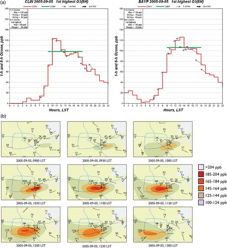
All days found using the four NTOC criteria were then analyzed, focusing on hourly spatial and temporal changes in observational data. Figure 6 shows an O₃ time series and contour plots of the highest measured 8-hr O₃ concentration at the BAYP and CLIN monitors. The time series shows the hourly averaged O₃ concentration in red and hourly resultant wind vectors in blue. The green line represents the peak 8-hr O₃ concentration, the 8-hr window that was used, and a black arrow shows the 8-hr resultant wind vector. The contour plots were generated by the TCEQ on the basis of interpolated concentrations observed at surface monitors.25 On this day, the CLIN monitor satisfies NTOC criteria 1–4, and the BAYP monitor satisfies NTOC criteria 2 and 4. In the case of BAYP, the maximum 8-hr O₃ time window was outside of the time of the 2-hr largest rise. At the bottom of this figure are snapshots of the O₃ contour animation showing a high-concentration plume starting to form between DRPK and Battleground Road and then heading toward a cluster of monitors near CLIN. Later in the day, its leading edge reached BAYP, causing a rapid 2-hr rise followed by a sustained multihour impact because the plume length was 4–5 times its width. Note that the plume was so narrow that monitors south of BAYP were not impacted.

Figure 6. O₃ (a) time series and (b) contour plots of the highest measured concentrations 8-hr O₃ concentration at the BAYP and CLIN monitors. The time series shows the hourly averaged O₃ concentration in red and hourly resultant wind vectors in blue. The green line represents the peak 8-hr O₃ concentration, the 8-hr window that was used, and a black arrow shows the 8-hr resultant wind vector. The contour plots were generated by the TCEQ on the basis of interpolated concentrations observed at surface monitors.25

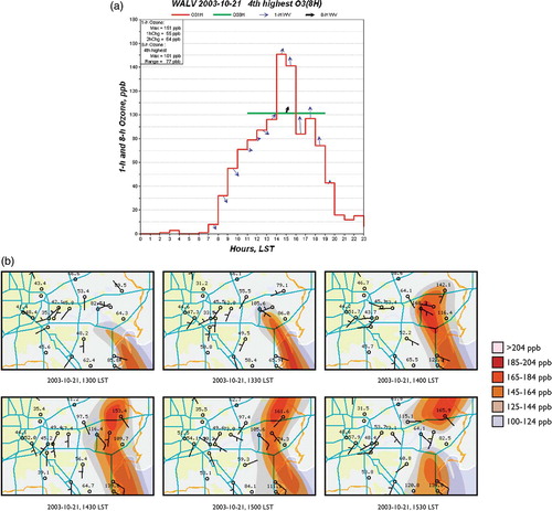
Figure 7 is an example of a case that satisfies all NTOC criteria for the WALV monitor. This is the fourth-highest annual 8-hr O₃ and is used in the DV_mfor this monitor. The 1-hr time series plot shows a large 1-hr increase of 55 ppb from 2:00 to 3:00 p.m. LST. This concentration spike, in the middle of already elevated O₃ values, was only 2 hr in duration at the monitor; the O₃ concentration decreased by 57 ppb 2 hr after the increase. Although the duration of this event was only 2 hr, its magnitude dramatically increases the 8-hr maximum O₃, making this day one of the top four highest observations of the year. Had the increase at 2:00 p.m. LST been only 13 ppb (the next greatest O₃ increase during the 8-hr time window), the daily maximum 8-hr average concentration would have been approximately 90 ppb and likely not the DV_m day at this monitor. Figure 7 shows that the O₃ plume is transported from the south to the WALV monitor. The concentration gradient within the narrow plume is high, which is consistent with the rapid increase in observed O₃ at the monitor. The timing of the animated plume strike and 1-hr peak from the time series is also in excellent agreement: both happen at 2:00 p.m. LST. Furthermore, the precipitous drop in O₃ seen in the time series plot occurs right after the plume has passed the monitor. As shown in the resultant wind vectors for WALV in Figure 2, the transport of high O₃ from the south occurs for every 8-hr O₃ concentration used in the DV_m calculation.

Figure 7. O₃ (a) time series and (b) contour plots of the highest measured concentrations 8-hr O₃ concentration at the WALV monitor. The time series shows the hourly averaged O₃ concentration in red and the ground-level hourly resultant wind vectors in blue. The green line represents the peak 8-hr O₃ concentration, the 8-hr window that was used, and a black arrow shows the 8-hr resultant wind vector. The contour plots were generated by the TCEQ on the basis of interpolated concentrations observed at surface monitors.25

The observational analysis shows that although some sites have had very large reductions in maximum O₃, O₃ plumes that originate near LaPorte and Bayport continue to impact several sites. The TCEQ generated O₃ contours plots for many events that also appear to originate near the Bayport area and are transported due north along the bay shore and right into WALV.25 These same figures also show that high O₃ observed at DRPK, HSMA, and BAYP are almost always due to narrow, high-O₃ plumes that originate near LaPorte/Bayport, often impacting or sideswiping DRPK, hitting HSMA, and later impacting or sideswiping BAYP. As shown in Figure 2, from 2003 to 2006, the 8-hr average ground-level wind vectors for the fourth-highest days at BAYP were from the east, identifying the ship channel as a possible source. In 2007 and 2008, the wind direction associated with the fourth-highest O₃ at BAYP shifted directions and the magnitude of the 8-hr O₃ also decreased significantly. This suggests that the sources causing the highest observed O₃ at BAYP have changed because of meteorological changes, effective emission reductions, or both.

The modeling scenarios used by the TCEQ include days that are recognized as NTOC days. Table 4 shows the dates of the observed top four highest 8-hr O₃ maxima for seven monitors for 2005 and 2006. Days in bold were classified as NTOCs, and the italics correspond to days that were simulated by TCEQ. In 2005, 2 of the 15 NTOC days were simulated, and in 2006, 9 of 10 NTOC days were simulated. In 2006, all four of the DRPK days were NTOC days and they were also simulated. If these NTOC days were impacted by emission events, the standard CAMx photochemical model using the typical baseline modeling inventory would not include these episodic emissions. Furthermore, if the model happened to produce a result that appeared to replicate the O₃ measurements on these days, this would surely be the result of compensating errors in the model and its input structures. Simply put, the standard regulatory modeling paradigm required by EPA cannot predict, for the right reasons, the 1-hr O₃ phenomena demonstrated here because the true cause-effect process phenomena do not exist in the modeling system.

Table 4. The dates (month/day) of the top four highest daily maximum 8-hr O₃ concentrations in ppb for 2005 and 2006 four seven monitors

	2005					2006
Sites	1st	2nd	3rd	4th	Total Simulated	1st	2nd	3rd	4th	Total Simulated
BAYP	09/05	08/02	06/21	06/22	3	08/31	06/29	09/07	06/28	2
HSMA	10/09	09/30	09/20	09/20	0	06/29	06/14	08/17	08/31	3
DRPK	07/08	08/21	10/17	06/22	1	09/01	06/08	08/17	06/12	4
WALV	06/02	08/21	10/18	07/11	1	06/05	06/04	06/08	06/10	4
HNWA	05/27	05/06	06/23	06/02	3	06/05	09/14	06/29	04/13	2
HALC	06/02	05/14	05/27	10/18	2	09/01	06/05	06/08	09/14	4
CLIN	09/05	10/17	08/01	10/12	0	06/29	09/01	08/31	09/07	3
Notes: The dates in bold were classified as having NTOCs, and the italic dates were days simulated by the TCEQ.

DISCUSSION

On the basis of the evidence presented in this work, parts of the O₃ problem in Houston cannot be effectively treated with EPA's current 8-hr O₃ modeling approach. However, this modeling approach is not a legal requirement and is simply guidance that can be altered with approval by the EPA. A plausible alternative approach would be to use the NTOC criteria to separate out those days and monitors that are better suited to be controlled by enforcement, or expansion of the existing short-term HRVOC rule, and to remove them from the DV_m calculation. By sorting the days at a monitor site and applying a protocol of tests and supporting evidence, the nontypical and the typical O₃ can be categorized. The nontypical O₃ days can be addressed by additional short-term rule-type actions, whereas the typical O₃ days can be treated by standard application of EPA's nominal photochemical modeling and emissions inventory guidance. Just such a dual-O₃ paradigm served as the technical foundation of the 2004 Houston 1-hr O₃ SIP mid-course review that was approved by the EPA.

Alternative Attainment Method

In this alternative method, the high-O₃ days that influence the DV_B,m for a monitor are first identified, and then the set of days are filtered to leave the typical ozone change (TOC) days. The term “natural” will be applied to the observational set without filtering, and the term “filtered” will be applied to the set that has NTOC days removed and the remaining TOC days moved up in the order. That is, the third-highest day in the natural set at a monitor may be a TOC day, but the first and the second natural day may be NTOC days. In this case, the first two days are set aside in a list of days to be regulated by the enhanced short-term rule, and the third-highest natural day becomes the first-highest filtered day. The process continues until 4 days that are only TOC-type days are found. The fourth-highest day of this filtered set becomes a part of the DV_m calculation for this monitor and is entered into the calculation of the DV_B,_m used in the attainment test.

Table 5 shows the calculation of the DV_F,m values at the four monitors. Only the DRPK monitor is predicted to remain above 80 ppb in 2018. These filtered DV_F,m values are close enough to 75 ppb that with improvements in the responsiveness of the model, they might be able to demonstrate attainment of the new 75-ppb standard. Supplemental Figures 2 and 3 compare the DV_m component plots for the natural and filtered days for years 2003–2008 at BAYP, WALV, DRPK, and HSMA. Most notable are the disappearance of the high 1-hr O₃ values, especially at DRPK and WALV.

Table 5. Listing of the monitors with the top four highest DV_F,m in ppb, their RRF, and the 2006 DV_B,m in ppb

Monitor	RRF	DVB,m	DVF,m	DVB,filtered	DVF,filtered	Difference
BAYP	0.900	96.7	87.0	88.7	79.8	−7.2
HSMA	0.934	90.3	84.3	82.3	76.9	−7.5
DRPK	0.958	92.0	88.1	86.3	82.7	−5.5
WALV	0.959	92.0	88.2	82.3	78.9	−9.3
Notes: Also shown are the recalculated 2006 DVB,filtered in ppb, where NTOC days were “filtered” from the dataset. The existing RRF values are multiplied by the DVB,filtered to calculate a new DVF,filtered. The difference in DVF,m is also shown (DVF,filtered – DVF,m).

This procedure logically follows from the conceptual model expressed in the 2004 SIP that led to an effective set of rules being adopted and resulted in unprecedented reductions of O₃ at monitors in as short of a time as 5 yr. Using observational analysis to bring the 2004 conceptual model and already-adopted and EPA-approved rules up to date to be consistent with 8-hr needs clearly falls within the weight-of-evidence domain.15

CONCLUSIONS

The commonly accepted “conceptual model” of gradual increases in O₃ concentrations and the means for O₃ control is a core element in EPA's O₃ attainment methodology. However, for Houston mounting evidence suggests that not all peak 1-hr and 8-hr O₃ concentrations of regulatory significance can be adequately explained by this traditional paradigm. When the EPA methodology is applied to Houston, the regulatory model is missing a critical cause for high O₃. This could be a plausible reason for why the model is not as responsive when compared with the real world. For example, ambient observations in Houston over the period 2007–2009 show that the area's measured O₃ DV_m had dropped below the 85-ppb standard, faster than the modeling results predicted. Furthermore, when attempting to construct future control requirements with the current regulatory approach, implausible attainment results are predicted. When regulatory modeling results are extrapolated to the levels of the expected lower NAAQS (60–70 ppb), the result is that only by eliminating virtually all industrial point-source NO_x and VOC emissions can Houston show attainment by 201824,28 Understanding the causes of high O₃ in Houston is critical to improving model performance.

There is a need to further understand all of the causes of peak 8-hr O₃ levels in Houston, simulate them correctly, and find the most cost-effective means for O₃ control. This work shows that observed spatial patterns in O₃ are not being predicted in the model and future work will focus on this issue. Model performance analysis is needed through trajectory29 and air mass30 analyses, process analysis,31–35 and source apportionment modeling experiments36 to more robustly link emission events of known or plausible location to measured and modeled O₃. Further study is also needed to understand how other processes (e.g., boundary layer transport phenomena) can influence NTOCs. Further examination of the ground-level wind quadrant analysis,31 in the context of the land-sea breeze circulations, air mass stagnation, and the seasonal evolution of regional-scale flow patterns, may shed additional light on the role that transport has for NTOCs.

ACKNOWLEDGMENTS

The authors thank Lola Brown, Mark Estes, Dick Karp, and Dr. Jim Smith from TCEQ for providing data and guidance. They also thank James Wilkinson of Alpine Geophysics for his assistance in the emission inventory analysis. The Texas Environmental Research Consortium through the Houston Advanced Research Center funded this work.

REFERENCES

- Banta , R.M. , Senff , C.J. , Nielsen-Gammon , J. , Darby , L.S. , Ryerson , T.B. , Alvarez , R.J. , Sanberg , S.P. , Williams , E.J. and Trainer , M. 2005 . A Bad Air Day in Houston , Bulletin of the American Meterological Society .
- Cowling , E. , Furiness , C. , Dimitriades , B. and Parrish , D. 2007 . Final Rapid Science Synthesis Report: Findings from the Second Texas Air Quality Study (TexAQSII)
- SIP Revision: Houston-Galveston-Brazoria: Ch. 101 and Ch. 115 Rules; Texas Commission on Environmental Quality: Austin, TX, 2004 http://www.tceq.state.tx.us/implementation/air/sip/dec2004hgb_mcr.html (http://www.tceq.state.tx.us/implementation/air/sip/dec2004hgb_mcr.html) (Accessed: 2010 ).
- 2004 . The State Implementation Plan for the Control of Ozone Pollution: Attainment Demonstration for the Houston/Galveston Ozone Non-attainment Area , Austin , TX : Texas Commission on Environmental Quality .
- Yarwood , G. , Ramsey , S.H. , Colville , C.J. and Bhat , S.B. 2008 . Cost Analysis of HRVOC Controls on Polymer Plants and Flares Project 2008–104 , Novato , CA : ENVIRON International Corporation .
- FLIR GF-Series Infrared Cameras; FLIR Systems: Boston, MA, 2010 http://www.flir.com/thermography/americas/us/content/?id=18296 (http://www.flir.com/thermography/americas/us/content/?id=18296) (Accessed: 2010 ).
- Forecast for Houston: Air Quality Improving. Natural Outlook 2008; Texas Commission on Environmental Quality: Austin, TX, 2008 http://www.tceq.state.tx.us/comm_exec/forms_pubs/pubs/pd/020/08-02/forecastforhouston.html (http://www.tceq.state.tx.us/comm_exec/forms_pubs/pubs/pd/020/08-02/forecastforhouston.html) (Accessed: 2010 ).
- Estes , M. , Harper , C.F. , Karp , D. and Jolly , J. 2006 . A New Spatial Emission Adjustment for HRVOCs , Houston , TX : Southeast Texas Photochemical Modeling Technical Committee .
- Hansen , S. Monitoring and Data Analysis Issue Area Report . Presented at the Houston Regional Monitoring Corporation 2009 Annual Members Meeting . Houston , TX .
- 2010 . Revision to the State Implementation Plan for the Control of Ozone Air Pollution Houston Galveston Brazoria 1997 Eight Hour Ozone Standard Nonattainment Area , Austin , TX : Texas Commission on Environmental Quality .
- 2009 . Houston-Galveston-Brazoria Eight-Hour Ozone SIP Modeling (2005, 2006 Episodes) , Austin , TX : Texas Commission on Environmental Quality .
- Parrish , D.D. , Allen , D.T. , Bates , T.S. , Estes , M. , Fehsenfeld , F.C. , Fein-gold , G. , Ferrare , R. , Hardesty , R.M. , Meagher , J.F. , Nielsen-Gammon , J.W. , Pierce , R.B. , Ryerson , T.B. , Seinfeld , J.H. and Williams , E.J. 2009 . Overview of the Second Texas Air Quality Study (TexAQS II) and the Gulf of Mexico Atmospheric Composition and Climate Study (GoMACCS) . J. Geophys. Res. Atmos. , 114 D00F13 doi: 10.1029/2009JD011842
- Yang , Y.J. , Stockwell , W.R. and Milford , J.B. 1995 . Uncertainties in Incremental Reactivities of Volatile Organic-Compounds . Environ. Sci. Technol. , 29 : 1336 – 1345 .
- Hogrefe , C. , Civerolo , K.L. , Hao , W. , Ku , J.Y. , Zalewsky , E.E. and Sistla , G. 2008 . Rethinking the Assessment of Photochemical Modeling Systems in Air Quality Planning Applications . Journal of the Air & Waste Management Association , 58 : 1086 – 1099 . doi: 10.3155/1047-3289.58.8.1086
- Jones , J.M. , Hogrefe , C. , Henry , R.F. , Ku , J.Y. and Sistla , G. 2005 . An Assessment of the Sensitivity and Reliability of the Relative Reduction Factor Approach in the Development of 8-hr Ozone Attainment Plans . Journal of the Air & Waste Management Association , 55 : 13 – 19 .
- Sistla , G. , Hogrefe , C. , Hao , W. , Ku , J.Y. , Zalewsky , E. , Henry , R.F. and Civerolo , K. 2004 . An Operational Assessment of the Application of the Relative Reduction Factors in the Demonstration of Attainment of the 8-hr Ozone National Ambient Air Quality Standard . Journal of the Air & Waste Management Association , 54 : 950 – 959 .
- 2007 . Guidance on the Use of Models and Other Analyses for Demonstrating Attainment of Air Quality Goals for Ozone,PM2.5, and Regional Haze , Research Triangle Park , NC : U.S. Environmental Protection Agency; Office of Air Quality Planning and Standards .
- Reynolds , S.D. , Roth , P.M. and Seinfeld , J.H. 1973 . Mathematical Modeling of Photochemical Air Pollution. 1. Formulation of Model . Atmos. Environ. , 7 : 1033 – 1061 .
- Lamb , R.G. and Seinfeld , J.H. 1973 . Mathematical Modeling of Urban Air-Pollution—General Theory . Environ. Sci. Technol. , 7 : 253 – 261 .
- Tesche , T.W. 1983 . Photochemical Dispersion Modeling: A Review of Model Concepts and Recent Applications Studies . Environ. Int. , 9 : 465 – 489 .
- Guideline for Regulatory Application of the Urban Airshed Model . EPA-450/4-91-013 . 1991 . U.S. Environmental Protection Agency; Office of Air Quality Planning and Standards: Research Triangle Park, NC
- Federal Register Rules and Regulation 40 CFR Parts 50 and 58 National Ambient Air Quality Standards for Ozone; Docket I.D. EPA-HQ-OAR-2005-0172; 73, 16436-16514 http://www.regulations.gov (http://www.regulations.gov)
- Hogrefe , C. and Rao , S.T. 2001 . Demonstrating Attainment of the Air Quality Standards: Integration of Observations and Model Predictions into the Probabilistic Framework . Journal of the Air & Waste Management Association , 51 : 1060 – 1072 .
- William , V. , Biton , L. , Jeffries , H.E. and Couzo , E. 2010 . Evaluation of Relative Response Factor Methodology for Demonstrating Attainment of Ozone in Houston, Texas . Journal of the Air & Waste Management Association , 60 : 838 – 848 . doi: 10.3155/1047-3289.60.7.838
- Kim , Y. , Fu , J.S. and Miller , T.L. 2010 . Improving Ozone Modeling in Complex Terrain at a Fine Grid Resolution: Part I. Examination of Analysis Nudging and All PBL Schemes Associated with LSMs in Meteorological Model . Atmos. Environ. , 44 : 523 – 532 .
- Zhang , Y. , Liu , X.-H. , Olsen , K.M. , Wang , W.-X. , Do , B.A. and Bridgers , G.M. 2010 . Responses of Future Air Quality to Emission Controls over North Carolina, Part II: Analyses of Future-Year Predictions and Their Policy Implications . Atmos. Environ. , 44 : 2767 – 2779 .
- Karp , D. 2009 . 2018 Future Year Matrix Modeling with 2006 Baseline Year NOX, VOC and NOX + VOC Reductions , Houston , TX : Southeast Texas Photochemical Modeling Technical Committee .
- Ozone Data; Texas Commission on Environmental Quality: Austin, TX, 2010 http://www.tceq.state.tx.us/nav/data/ozone_data.html (http://www.tceq.state.tx.us/nav/data/ozone_data.html) (Accessed: 2010 ).
- 2009 . User's Guide CAMx Comprehensive Air Quality Model with Extensions , Novato , CA : ENVIRON International Corporation .
- Allen , D. , Murphy , C. , Kimura , Y. , Vizuete , W. , Edgar , T. , Jeffries , H.E. , Kim , B.-U. , Webster , M. and Symons , M. 2004 . Final Report Texas Environmental Research Consortium Project H13: Variable Industrial VOC Emissions and Their Impact on Ozone Formation in the Houston Galveston Area , The Woodlands , TX : Houston Advanced Research Center .
- Karp , D. Initial 2018 HGB Modeling Results . Presented at the Southeast Texas Photochemical Modeling Technical Committee . Houston , TX .
- Sullivan , D. 2009 . Effects of Meteorology on Pollutant Trends , Austin , TX : University of Texas–Austin .
- Davis , R.E. , Normile , C.P. , Sitka , L. , Hondula , D.M. , Knight , D.B. , Gawtry , S.P. and Stenger , P.J. 2010 . A Comparison of Trajectory and Air Mass Approaches to Examine Ozone Variability . Atmos. Environ. , 44 : 64 – 74 .
- Vizuete , W. , Jeffries , H. , Valencia , A. , Couzo , E. , Christoph , E. , Wilkinson , J. , Henderson , B. , Parikh , H. and Kolling , J. 2009 . HARC Project H97: Multi-Model, Multi-Episode Process Analysis to Investigate Ozone Formation and Control Sensitivity in the 2000/2005/2006 Houston SIP Episode Models , The Woodlands , TX : Houston Advanced Research Center .
- Olaguer , E. , Rappengluck , B. , Lefer , B. , Stutz , J. , Dibb , J. , Griffind , R. , Brunee , B. , Shauck , M. , Buhrg , M. , Jeffries , H. , Vizuete , W. and Pinto , J. 2009 . Deciphering the Role of Radical Sources during the Second Texas Air Quality Study . Journal of the Air & Waste Management Association , 59 : 1258 – 1277 . doi: 10.3155/1047-3289.59.11.1258
- Kimura , Y. , McDonald-Buller , E. , Vizuete , W. and Allen , D.T. 2008 . Application of a Lagrangian Process Analysis Tool to Characterize Ozone Formation in Southeast Texas . Atmos. Environ. , 42 : 5743 – 5759 .
- Song , J. , Vizuete , W. , Chang , S. , Allen , D. , Kimura , Y. , Kemball-Cook , S. , Yarwood , G. , Kiournourtzoglou , M.A. , Atlas , E. , Hansel , A. , Wisthaler , A. and McDonald-Buller , E. 2008 . Comparisons of Modeled and Observed Isoprene Concentrations in Southeast Texas . Atmos. Environ. , 42 : 1922 – 1940 .
- Vizuete , W.V. , Kim , B.U. , Jeffries , H.E. , Kimura , Y. , Allen , D.T. , Kioumourtzoglou , M. , Biton , L. and Henderson , B. 2008 . Modeling Ozone Formation from Industrial Emission Events in Houston, Texas . Atmos. Environ. , 42 : 7641 – 7650 .
- Kemball-Cook , S. , Parrish , D. , Ryerson , T. , Nopmongcol , U. , Johnson , J. , Tai , E. and Yarwood , G. 2009 . Contributions of Regional Transport and Local Sources to Ozone Exceedances in Houston and Dallas: Comparison of Results from a Photochemical Grid Model to Aircraft and Surface Measurements . J. Geophys. Res. Atmos. , 114 D00F02 doi: 10.1029/2008JD010248