Modeling Transit Bus Fuel Consumption on the Basis of Cycle Properties

ABSTRACT

A method exists to predict heavy-duty vehicle fuel economy and emissions over an “unseen” cycle or during unseen on-road activity on the basis of fuel consumption and emissions data from measured chassis dynamometer test cycles and properties (statistical parameters) of those cycles. No regression is required for the method, which relies solely on the linear association of vehicle performance with cycle properties. This method has been advanced and examined using previously published heavy-duty truck data gathered using the West Virginia University heavy-duty chassis dynamometer with the trucks exercised over limited test cycles. In this study, data were available from a Washington Metropolitan Area Transit Authority emission testing program conducted in 2006. Chassis dynamometer data from two conventional diesel buses, two compressed natural gas buses, and one hybrid diesel bus were evaluated using an expanded driving cycle set of 16 or 17 different driving cycles. Cycle properties and vehicle fuel consumption measurements from three baseline cycles were selected to generate a linear model and then to predict unseen fuel consumption over the remaining 13 or 14 cycles. Average velocity, average positive acceleration, and number of stops per distance were found to be the desired cycle properties for use in the model. The methodology allowed for the prediction of fuel consumption with an average error of 8.5% from vehicles operating on a diverse set of chassis dynamometer cycles on the basis of relatively few experimental measurements. It was found that the data used for prediction should be acquired from a set that must include an idle cycle along with a relatively slow transient cycle and a relatively high speed cycle. The method was also applied to oxides of nitrogen prediction and was found to have less predictive capability than for fuel consumption with an average error of 20.4%.

IMPLICATIONS

It is unclear what direction the next major regulation will take, but greenhouse gas emissions are at the forefront of concern for mobile power sources. From a regulatory perspective for inventory purposes or from that of a fleet owner for reducing costs, a robust but simple model for estimation of fuel consumption is desired. This study developed a modeling methodology to predict the fuel consumption of a vehicle exercised over unseen cycles using limited chassis dynamometer data, reducing heavy-duty chassis dynamometer costs. This approach may also help to compare emissions or fuel economy between vehicles that were not tested over the same set of driving cycles.

INTRODUCTION

The primary emissions species of concern from heavy-duty diesel engines in on-road commercial vehicles have been particulate matter and oxides of nitrogen (NO_x), and these two exhaust species have been reduced by nearly 2 orders of magnitude since the late 1980s in the United States. It is unclear what direction the next major regulation in the United States and elsewhere will take, but greenhouse gas emissions are currently at the forefront of concern. Furthermore, there is a drive to improve fuel efficiency to conserve resources and bolster national security. The conversion of energy from a hydrocarbon fuel (e.g., diesel or natural gas) during combustion results in carbon dioxide (CO₂) being produced, and the amount of CO₂ emitted is inversely proportional to the conversion efficiency. Similarly, a vehicle's fuel economy (distance traveled per fuel consumed) is inversely proportional to the CO₂ mass rate. With heavy-duty diesel engines dominating the transportation sector and being a major source for CO₂ production, a reduction in fuel consumption, or an improvement in fuel economy, will result in less CO₂ being emitted into the atmosphere.

From a modeling perspective, from a regulatory perspective for inventory purposes or a from a fleet owner perspective for reducing costs, a robust but simple model is desired. A linear model was proposed by Clark et al.1 to predict emissions emitted by a vehicle exercised over an “unseen” chassis dynamometer cycle on the basis of data from other chassis dynamometer cycles using metrics of the cycles. This model was further detailed by Delgado et al.2 using additional metrics and focused on the fuel economy prediction capabilities of the model. The motivation for this modeling approach was to predict the emissions or fuel economy of a vehicle exercised over new or unseen cycles using limited chassis dynamometer data so as to reduce heavy-duty chassis dynamometer operation costs. This approach may also help to compare emissions or fuel economy between vehicles or technologies that were not tested over the same set of driving cycles. Although other methods exist for predicting emissions or fuel consumption for unseen vehicle activity,3–7 they generally require second-by-second emissions data or detailed knowledge of vehicle hardware and control strategies. The modeling approach discussed in this paper only requires aggregated emissions (average values over a cycle) and parameters calculated from the speed-time profiles.

This paper is directed toward developing and verifying a mathematical-empirical methodology for predicting heavy-duty vehicle fuel consumption during operation over unseen chassis dynamometer driving cycles on the basis of fuel consumption data that were gathered from operation on known chassis dynamometer cycles and properties of those cycles. The methodology allowed for the prediction of fuel consumption from vehicles operating on several different chassis dynamometer cycles on the basis of relatively few experimental measurements. West Virginia University (WVU) Center for Alternative Fuels, Engines, and Emissions heavy-duty chassis dynamometer data gathered from the Washington Metropolitan Area Transit Authority (WMATA) emission testing program8,9 were used to examine the method over an expanded number of chassis test cycles.

BACKGROUND

Road Load Equation

Vehicle fuel consumption depends on vehicle power demand as the vehicle is driven. The power requirement for a given vehicle can be calculated from the road load equation, which includes rolling resistance, aerodynamic drag, and inertial power required to accelerate the vehicle. Equation 1 shows the road load equation, where P represents the propulsion power demanded by the vehicle at the drive wheels, m is the mass of the vehicle, ρ represents the coefficient of rolling resistance, g is the acceleration because of gravity, V is the instantaneous velocity, ρ is the ambient air density, A is the frontal cross-sectional area of the vehicle, C _D is the aerodynamic drag coefficient, and t is time. Rotational inertia of the wheels, tires, and axles may be taken into account by adding an equivalent mass to the vehicle's total mass, but it has been neglected here because it was assumed as approximately 5% contribution.10 Road grade will also have an effect on vehicle power demand. Chassis dynamometer testing is usually executed assuming that level grade and road grade have been excluded.

(1)

Cycle Properties

A chassis dynamometer test cycle is customarily defined as a speed versus time array assuming a level road. A cycle has a defined test duration and target distance. A useful way to characterize a cycle is by means of cycle properties, or metrics, such as average velocity, standard deviation of velocity, average acceleration, and stops per distance. These metrics provide some information that the speed-time trace cannot give by itself. The most important metric to analyze fuel consumption is believed to be the average velocity because in eq 1 velocity appears in each term. Average velocity is a robust indicator of the type of activity exhibited during a given cycle. A low average velocity may represent a very transient cycle similar to what is expected in city traffic, whereas a high average velocity may represent a more steady behavior similar to what is expected in highway driving.

The main hypothesis of this research was that one might use cycle metrics to predict (with acceptable accuracy) the fuel consumption from a vehicle exercised through an unseen speed-time trace. The road load equation and the discussion above suggest that average velocity should be one of the metrics to be used; however, two different types of activity can be represented by the same value of average velocity, and another metric should be introduced to account for transient behavior. Average positive acceleration was selected for this purpose on the basis of previously published results.2,11 Note that other important properties such as standard deviation of speed, percentage of time idling, or stops per distance can be also taken into account to analyze fuel consumption. Vehicle-specific power is consistently identified as an explanatory variable that is highly correlated with emissions3 and may be another suitable cycle property to analyze fuel consumption. Note that transient vehicle operation implies transient engine operation, and for engines with cooled exhaust gas recirculation, emissions and fuel efficiency may be affected by the degree of transient behavior, even at the same instantaneous power level.

METHODS

Overview

A method for predicting emissions data for transient vehicle activity (such as a chassis dynamometer test cycle or in-use data) on the basis of information from measured chassis dynamometer test cycles has been identified and developed. The technique was presented by Taylor et al.12 and involves identifying the most important properties (metrics) of a cycle and developing a technique that proportions emissions for an unseen cycle on the basis of emissions from cycle data using those metrics for weighting. Using the same approach, this research predicted fuel consumption for a given vehicle over an unseen cycle as a linear combination of measured fuel consumption from a set of baseline cycles using an expanded set of test cycles. The weighting factors for the linear combination of cycles were determined by posing a simultaneous set of equations on the basis of cycle properties. In this way each baseline cycle will contribute to a percentage of the fuel consumption of the unseen cycle. The number (N) of baseline test cycles determines the number of simultaneous equations and hence the number of properties that can be used. One of the equations will always constrain the sum of the coefficients to be equal to 1, so there will be N − 1 properties that are used to solve the N simultaneous equations. In each case, the predicted fuel consumption (CO₂ emissions mass rate in g/sec as a surrogate) would be a weighted summation of the fuel consumption from the baseline cycles, with the weighting coefficients constrained to sum to unity.

Method Description

Assume that fuel consumption measurements (cycle averaged CO₂ emissions in g/sec) for three different test cycles are available and one wants to estimate fuel economy for a fourth, different cycle. The three measured cycles are termed the “baseline cycles” and the predicted cycle is termed an “unseen cycle.” The baseline cycles form the basis to estimate fuel economy for the unseen cycle. Each baseline cycle will have a weighting factor (w) that defines the relative proportion of that cycle to the unseen cycle in terms of the metrics used. It is expected that these weighting factors can also be used to estimate the unseen cycle fuel economy. Two cycle properties should be used for a unique solution because the number of baseline cycles is 3.

The prediction method consists of posing a set of three simultaneous equations, on the basis of the selected cycle properties, to calculate the weights of each baseline cycle to the unseen cycle. The three unknowns are the weighting factors for each baseline cycle. The equation set is shown in matrix form in eq 2. The first two equations are linear combinations using two different metrics. The first equation uses average velocity (V), the second equation uses average acceleration (A), and the third equation constrains the weights to sum to 1. Note that other metrics and a different number of metrics (and baseline cycles) may have been used in the method.

(2)

The next step is to solve the simultaneous equations to obtain the weighting factors. Once the weighting factors are calculated, they are used to calculate fuel consumption (FC) for the unseen cycle as shown in eq 3.

(3)

Geometric Explanation

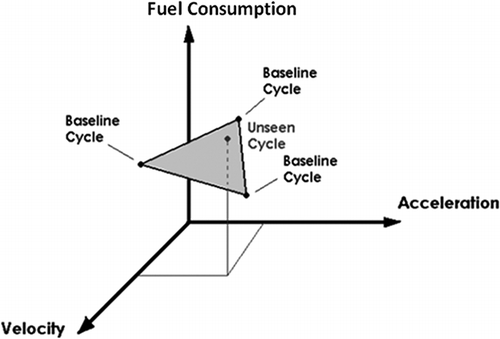
Solving a system of three equations and three unknowns as shown in the previous example is equivalent to finding the equation of a plane in a three-dimensional space. Figure 1 shows a geometric representation of the previous example. In this case, the dimensions of the three-dimensional space are average velocity, average acceleration, and fuel consumption. Information for each baseline cycle represents a point in that three-dimensional space. Once the three points have been specified, a plane that crosses the three points (unless the points are collinear) can be defined. This plane is unique because one and only one plane can cross through these three points. The plane can be used to predict other cycle's fuel economy a priori by just knowing these new cycle's properties (average velocity and average acceleration in this example). This modeling approach simplifies the real-world surface (which may be curvilinear) to a plane using minimum information. The prediction may use extrapolation (points on the plane but outside the triangle shown); however, as with other linear models, extrapolation should be exercised with caution.

Figure 1. Geometric interpretation of the linear model method.

Note that no regression technique is required for the method, which relies solely on the linear association of vehicle emissions with activity parameters. However, the key to successful prediction is the adequate selection of cycle properties and baseline cycles to be used in the model.

Data Used

The method was applied using previously published data gathered using the WVU heavy-duty chassis dynamometer. The data were available from the WMATA emission testing program in 2006.8,9 Chassis dynamometer data from two conventional diesel buses, two compressed natural gas (CNG) buses, and one hybrid diesel bus tested over 16 or 17 different driving cycles were used to verify the method with regard to fuel type, drive train configu-ration, and selected baseline test cycles. Cycle properties and vehicle fuel consumption measurements from three baseline cycles were selected to generate a linear model and then to predict unseen fuel consumption over the remaining 13 or 14 cycles. Average velocity and average positive acceleration were used as cycle properties in the model; it was assumed that negative acceleration (deceleration) events were not fueling conditions and hence zero emissions were produced. For each bus, all possible combinations of three baseline cycles were used to predict CO₂ mass rate (g/sec) over the remaining 13 or 14 cycles. A total of 3040 predictions were made, including 560 combinations among 16 cycles for three buses and 680 combinations among 17 cycles for two buses. The method was also applied to predict fuel economy (mpg) and NO_x mass rate emissions (g/sec).

Table 1 provides information on the buses. Table 2 shows the available cycles and average measured properties of velocity, acceleration, and stops per distance. The properties were determined from the actual speed-time values for each cycle. Target values were not used because differences in driving behavior are known to produce differences in emissions.13 However, for the unseen cycle, the target value must be used. In some applications in which the vehicle may be unable to follow the target cycle, the target cycle might be modified to estimate the most likely activity that the vehicle would actually demonstrate. Additional information on cycles and the WMATA program can be found elsewhere.8,9

Table 1. Transit buses analyzed in this research

Bus ID	Technology	Manufacturer	Bus Type and Model Year	Engine Type and Model Year	Gross Vehicle Weight (kg)	Available Cycles
32	CNG	John Deere	Orion 2005	RG6081 2005	19,334	16
35	CNG	Cummins	Orion 2005	Cummins CG 2005	19,334	16
37	Hybrid	Allison	New Flyer 2005	Cummins ISL280 2005	18,416	16
39	Diesel	DDC	Orion 1992	DDC S50 2003	17,896	17
41	Diesel	Cummins	New Flyer 2006	Cummins ISM280 2006	18,416	17

Table 2. Average measured properties over five buses for 17 cycles used

Number	Cycle Name	Cycle ID	Velocity (mph)	Acceleration (mph/sec)	Stops/Distance (stops/mi)
1	CARB Idle Cycle	Idle	0.06	0.00	0.00
2	New York Bus Cycle	NYBus	3.54	0.25	18.71
3	Paris Cycle	PARIS	6.68	0.32	12.40
4	Manhattan Cycle	Manhattan	6.86	0.37	9.76
5	Washington Metro Transit Authority Cycle	WMATA	8.43	0.30	6.26
6	New York Composite Cycle	NY-Comp	8.75	0.15	7.21
7	Orange County Transit Authority Cycle	OCTA	12.22	0.41	4.87
8	Central Business District Cycle	CBD	13.08	0.52	6.80
9	Braunschweig Cycle	BRAUN	13.88	0.45	4.19
10	City Suburban Heavy Vehicle Cycle	CSHVC	14.02	0.27	2.29
11	Beeline Cycle	Beeline	14.03	0.43	3.73
12	European Test Cycle Urban	ETCURBAN	14.11	0.28	1.92
13	CARB Transient Cycle	TRANS	15.33	0.28	1.69
14	Urban Dynamometer Driving Schedule	UDDS	18.71	0.20	2.04
15	King County Metro Cycle	KCM	23.35	0.41	1.85
16	Arterial Cycle	ART	25.58	0.55	1.47
17	Commuter Cycle	COMM	44.37	0.18	0.17

Goodness-of-Fit Criteria

Four criteria were selected to evaluate the goodness of fit between the measured and predicted fuel consumption data: average percentage error (eq 4, where x _p are predicted values and x _e are experimental values), maximum absolute error, average absolute error (eq 5, where x _p are predicted values and x _e are experimental values), and R ² correlation coefficients between the measured and predicted values.

(4)

(5)

RESULTS

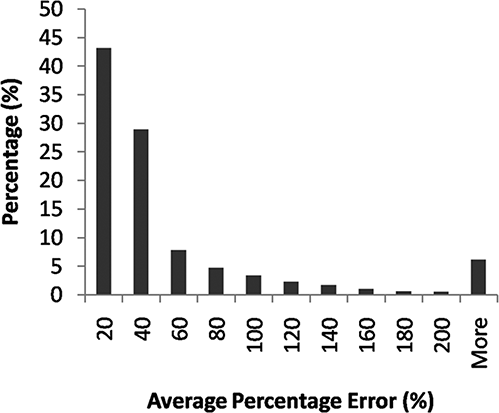
The key to successful prediction is the adequate selection of cycle properties and baseline cycles to be used in the model. In this way, it was expected that not all combinations of baseline cycles were suitable to perform a good prediction. Figure 2 illustrates this fact through a histogram of average percent error (among 13 or 14 predicted cycles) for CO₂ mass rate prediction. Approximately 44% of the combinations produced errors less than 20%, whereas approximately 6% of the combinations produced errors above 200%. The method is not suitable if the cycles are ill chosen. For example, using two very low average velocity cycles plus idle to predict high-speed behavior is fraught with difficulty that would be exacerbated if a poor combination of metrics were chosen.

Figure 2. Histogram of average percentage error for the prediction of CO₂ mass rate (g/sec).

Tables 3 and 4 show the predictions with the lowest average percent error for each bus for CO₂ mass rate and fuel economy, respectively. These tables show the baseline cycles used, average percentage error, average absolute error, maximum error, standard deviation of error, and R ² correlation coefficients between the measured and predicted values. Note that the idle cycle is present in the predictions with the lowest error for all vehicles. CO₂ prediction errors were below 8.88% whereas fuel economy prediction errors were at best 15.89%. The prediction of CO₂ mass rate showed a tendency to be a better method of prediction than a direct fuel economy prediction. This stems from the fuel economy at idle being equal for all vehicles (a value of zero by definition), whereas CO₂ mass rate for the idle cycle was different (and nonzero) for each vehicle. Using CO₂ mass rate provides additional information in the model. It is recommended that the prediction of fuel economy be done in terms of CO₂ and then convert to fuel economy, as was found by Clark et al.1 and Delgado et al.2 This paper will focus on CO₂ mass rate predictions rather than fuel economy predictions.

Table 3. CO₂ mass rate prediction results with lowest average percent error

Bus ID	Cycle 1	Cycle 2	Cycle 3	Percent Error	Average Error (g/sec)	Max Error (g/sec)	SD Error (g/sec)	R ^2
32	Idle	Beeline	KCM	8.48	0.54	1.12	0.37	0.92
35	Idle	PARIS	WMATA	7.53	0.53	1.20	0.37	0.95
37	Idle	OCTA	KCM	8.17	0.51	1.29	0.40	0.98
39	Idle	KCM	ART	8.70	0.83	2.45	0.68	0.93
41	Idle	PARIS	KCM	8.88	0.76	2.33	0.65	0.93
Notes: Metrics used: average velocity and average acceleration.

Table 4. Fuel economy predictions with lowest average percent error

Bus ID	Cycle 1	Cycle 2	Cycle 3	Percent Error	Average Error (mpg)	Max Error (mpg)	SD Error (mpg)	R ^2
32	Idle	Manhattan	OCTA	15.89	0.67	2.61	0.67	0.77
35	Idle	BRAUN	KCM	19.73	0.70	1.57	0.58	0.60
37	Idle	OCTA	COMM	22.26	1.19	2.43	0.93	0.18
39	Idle	Manhattan	KCM	20.34	0.85	2.12	0.76	0.38
41	Idle	Manhattan	KCM	22.17	1.01	2.19	0.77	0.39
Notes: Metrics used: average velocity and average acceleration.

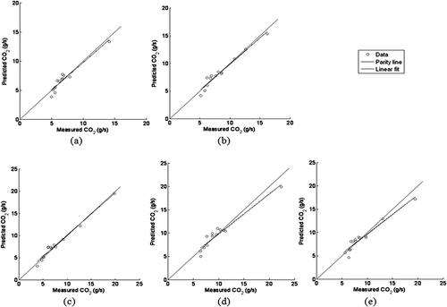
Note that most of the combinations presented in Table 3 include a cycle with a relatively high average velocity such as COMM, ART, KCM, or UDDS and a transient cycle with relatively low average velocity such as WMATA, Paris, or OCTA (see Table 2 for cycle names and IDs). The KCM cycle appears to be valuable because it worked relatively well as a low-speed cycle or as a high-speed cycle depending on the baseline cycle combination. Parity plots of measured versus predicted values for the lowest average percentage error for the prediction of CO₂ mass rate are shown in Figure 3. Figures 3a–3e represent the cases shown in Table 3 for buses 32, 35, 37, 39, and 41, respectively. On the basis of the results shown in Figure 3c, the hybrid vehicle can be modeled using the linear modeling methodology presented here. However, additional hybrid vehicles and hybrid vehicle architecture will need to be investigated to substantiate this claim. For diesel transit buses (Figure 3, d and e), fuel consumption was underpredicted for the COMM cycle because of extrapolation (predicting a cycle with higher average velocity than the baseline cycle with the highest average velocity) and this brought the linear regression line down for the CO₂ mass rate plot, causing the slope in the regression line to be less than 1. However, it appears that as long as a high-speed cycle was used as a baseline cycle, the extrapolation would not produce significant deviations between the measured and estimated values. CNG bus 35 (Figure 3b) illustrated an exception to this observation. The lowest error for bus 35 was obtained when using baseline cycles idle, Paris, and WMATA. The highest average velocity baseline cycle in this case was 8.43 mph for the WMATA cycle and the model was able to predict the COMM cycle with an average velocity of 44.37 mph within 1.12 g/sec. In this case, higher average speed extrapolation was possible.

Figure 3. CO₂ mass rate predictions with lowest error for (a) CNG bus 32, (b) CNG bus 35, (c) hybrid bus 37, (d) diesel bus 39, and (e) diesel bus 41.

Baseline Cycle Analysis

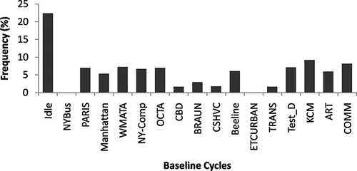
The key to obtaining a prediction with low error is the selection of suitable combinations of baseline cycles. A given baseline cycle is not “good” or “bad” by itself. Rather, it is the combination of individual baseline cycles that makes the predictive approach suitable or not. Also, a baseline cycle can have low errors with some metrics but have high errors with other metrics. Further, the success of the approach may vary according to the application because in some cases the best average prediction for a fleet of vehicles may be the objective, whereas in other applications there may be a need to constrain the worst individual error in the prediction. To this end, an analysis was performed to identify which cycles are more associated with predictions with low errors using average velocity and average acceleration. Figure 4 shows a histogram of the frequency of a given cycle in the combinations with percentage error less than 10%. The analysis was done using the CO₂ mass rate data. The plot shows that the idle cycle was present in more than 20% of the predictions. Idle activity is a desirable baseline cycle in this kind of modeling because it represents the case with minimum fuel consumption (under the no-grade constraint) for a given vehicle. Paris, WMATA, and OCTA cycles seem to be appropriate low-velocity baseline cycles, and KCM, UDDS, and COMM seem to be appropriate candidates as high-velocity baseline cycles. Note also that cycles like ETCURBAN or NYBus are not present in any combination with error less than 10%. The distinctive characteristic of these cycles with respect to other low-velocity cycles is that their values of average positive acceleration are relatively low (<0.3 mph/sec).

Figure 4. Frequency of a baseline cycle in predictions with average <10%.

Baseline Combination Analysis

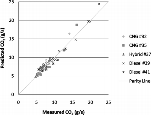
The three combinations of baseline cycles with the lowest errors for the prediction of CO₂ mass rate for the five buses considered are shown in Table 5. These combinations produced prediction results with less than 10% average error for all buses over a very wide range of cycles. The combination of idle cycle, a relatively low average speed with high average acceleration cycle (OCTA or PARIS), and a relatively high-speed cycle (KCM or COMM) was present in the three combinations. The best combination of baseline cycles in terms of average percentage error was idle, OCTA, and KCM cycles. The results of the combination are shown in Figure 5.

Table 5. Baseline combinations with lower average percentage error for CO₂ (g/sec) prediction

Baseline Cycles Used	Average Percent Error					Average Percent Error	Max Absolute Error (g/sec)
	CNG 32	CNG 35	Hybrid 37	Diesel 39	Diesel 41
Idle OCTA KCM	8.61	7.78	8.17	8.75	9.26	8.51	3.95
Idle PARIS KCM	9.11	7.55	8.89	8.72	8.88	8.63	3.18
Idle OCTA COMM	8.52	7.80	8.38	9.21	9.80	8.74	2.20
Notes: Metrics used: average velocity and average acceleration.

Figure 5. Parity plot for prediction of CO₂ mass rate using idle, OCTA, and KCM as baseline cycles and velocity and acceleration as metrics.

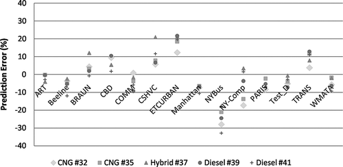
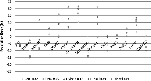
Figure 6 further illustrates how the combination of idle, OCTA, and KCM cycles predicted the other cycles with high fidelity and could be useful for seeing when fuel consumption for one cycle is consistently overpredicted or underpredicted. For example, it can be seen that CBD, CSHVC, ETCURBAN, and transient cycles' fuel consumption were overpredicted for all of the buses. The COMM cycle fuel consumption was mostly underpredicted (particularly for the diesel buses) because extrapolation appeared to be unable to account for the aerodynamic drag portion of the road load equation.

Figure 6. CO₂ mass rate prediction errors using idle, OCTA, and KCM as baseline cycles and average velocity and average acceleration as metrics.

Alternative Metrics

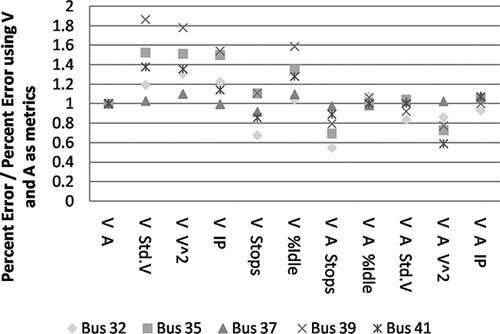
An exploratory analysis was completed to discern if other metrics had the potential to replace acceleration or to be used in conjunction with velocity and acceleration to obtain improved results. Figure 7 shows the ratio of average percentage error for alternative metrics over average percentage error using velocity and acceleration. A value less than 1 for this ratio meant that the alternative metrics combination had the potential to have lower errors than the velocity and acceleration combination alone. It can be seen that stops per distance (stops per mile) and average of velocity squared are metrics that could reduce the error when compared with using just the velocity and acceleration metrics. The information provided in this plot also shows that the accuracy of prediction could be improved by adding one more metric to the analysis but at the cost of adding one more baseline cycle; this is counter to the basic premise in the development of this approach. Only the best possible case (the case with minimum average percent error) was used for this analysis and further research should be done to validate these conclusions. The next section shows a more detailed analysis using stops per distance as an alternative metric.

Figure 7. Percentage error ratios when using other metrics combinations. V = velocity, A = acceleration, Std.V = standard deviation of speed, Stops = stops per unit distance, IP = inertial power.

Using Stops per Distance as a Metric

On the basis of the results shown in Figure 7, the bus data were modeled using the velocity and stops per distance metrics with different combinations of three baseline cycles. The results with the lowest prediction errors are shown in Table 6. The average percentage errors in the prediction of CO₂ mass rate (g/sec) are from 6.1% to 9.6% for individual buses. These results are about the same order of magnitude of those reported in Table 3 (7.5–8.9% error for individual buses). Note again that the idle cycle is present in all of the combinations with the lowest error.

Table 6. CO₂ mass rate prediction results with lowest average percentage error

Bus ID	Cycle 1	Cycle 2	Cycle 3	Average Percent Error	Average Error (g/sec)	Max Absolute Error (g/sec)	SD Error (g/sec)	R ^2
32	Idle	NYBus	CBD	6.08	0.47	1.89	0.49	0.97
35	Idle	NYBus	KCM	8.99	0.77	2.55	0.63	0.94
37	Idle	NYBus	WMATA	6.56	0.46	1.23	0.41	0.98
39	Idle	PARIS	UDDS	9.55	0.94	1.85	0.45	0.95
41	Idle	NYBus	COMM	7.82	0.59	1.42	0.51	0.89
Notes: Metrics used: velocity and stops per distance.

The idle, NYBus, and KCM combination of baseline cycles resulted in the lowest error for the bus data when the number of stops per distance metric was used. Figures 8 and 9 show the prediction results in detail. Note that when using velocity and acceleration as metrics, the best combination of baseline cycles was idle, OCTA, and KCM, and when using velocity and stops per distance as metrics, the best combination of baseline cycles was idle, NYBus, and KCM. The NYBus cycle was not a good baseline cycle when using average acceleration but was one of the best cycles when using stops per distance. Perhaps the fact that such a cycle is the one with the highest number of stops per distance helped the model to cover a wider envelope of vehicle operation.

Figure 8. Parity plot for prediction of CO₂ mass rate using idle, NYBus, and KCM as baseline cycles and velocity and stops per distance as metrics.

Figure 9. CO₂ mass rate prediction errors using idle, NYBus, and KCM as baseline cycles and average velocity and stops per distance as metrics.

Using an Additional Metric

The data were also evaluated using velocity, acceleration, and stops per distance using different combinations of four baseline cycles. Table 7 shows the results with the lowest errors for this case. It is worth mentioning that the idle cycle was still present in all of the cases. The use of an additional metric reduced the average error in the prediction of CO₂ mass rate (average error range from 4.92% to 8.15% for individual buses, compared with a 7.53–8.88% error range using just two metrics) but at the cost of having to test the vehicle over an additional cycle. On the basis of these results, the authors recommend using three baseline cycles to minimize the number of required tests and to reduce the model complexity. However, it may be beneficial in some cases to warrant additional testing to incrementally improve the model prediction.

Table 7. CO₂ mass rate prediction results with lowest average percentage error

Bus ID	Cycle 1	Cycle 2	Cycle 3	Cycle 4	Average Percent Error	Average Error (g/sec)	Max Absolute Error (g/sec)	SD Error (g/sec)	R ^2
32	Idle	NYBus	BRAUN	COMM	4.92	0.32	0.55	0.19	0.91
35	Idle	NYBus	WMATA	COMM	5.65	0.40	1.13	0.33	0.94
37	Idle	NYBus	PARIS	UDDS	6.97	0.48	1.23	0.42	0.98
39	Idle	NYBus	BRAUN	KCM	6.82	0.63	1.63	0.42	0.98
41	Idle	Manhattan	OCTA	UDDS	8.15	0.63	1.33	0.45	0.97
Notes: Metrics used: average velocity, average acceleration, and stops per distance.

NO_x Prediction

The method was also applied to predict NO_x mass rate emissions in grams per second. Average velocity and average positive acceleration were used as metrics. No attempt was made to increase the accuracy of the method using a more diverse set of metrics. Table 8 shows the lowest error combinations obtained for each bus. Engine technology seems to have an effect on the quality of the prediction. CNG buses' NO_x prediction resulted in higher percentage errors when compared with diesel buses (CNG bus 32 with ∼28% error, CNG bus 35 with ∼15% error, compared with ∼10% error for diesel buses 39 and 41). This may be occurring because of the high sensitivity of CNG engines' NO_x emissions to air-to-fuel ratios.14 The hybrid bus NO_x prediction had percentage errors about the same order of magnitude of CO₂ prediction errors (∼8%).

Table 8. NO_x mass rate prediction with lowest average percentage error

Bus ID	Cycle 1	Cycle 2	Cycle 3	Average Percent Error	Average Error (g/sec)	Max Error (g/sec)	SD Error (g/sec)	R ^2
32	Idle	CSHVC	COMM	27.76	0.015	0.047	0.013	0.03
35	Idle	ETCURBAN	COMM	14.93	0.011	0.042	0.013	0.29
37	Idle	WMATA	Trans	8.01	0.004	0.017	0.005	0.97
39	Idle	KCM	COMM	10.28	0.005	0.014	0.004	0.58
41	NY-Comp	CBD	ART	10.34	0.003	0.029	0.007	0.58
Notes: Metrics used: average velocity and average acceleration.

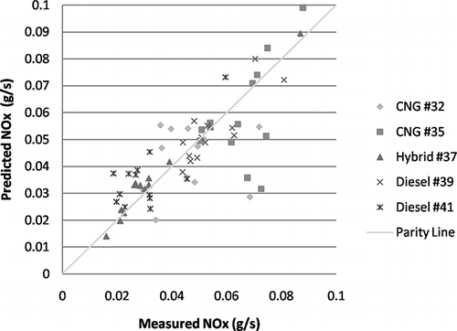
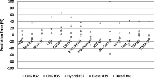
The combination idle, OCTA, and KCM was evaluated for prediction of NO_x using average velocity and average acceleration as metrics. Figure 10 shows a parity plot of NO_x emission mass rate measured versus predicted values for all of the predictions. Individual errors per cycle are illustrated in Figure 11. It can be seen that most of the predictions are within a percentage error range of ±60% (absolute error of ∼0.02 g/sec). Overall results are poorer than the previous CO₂ prediction (with an average NO_x rate error of 20.4% over the five buses compared with ∼10% for CO₂). Keep in mind that the method relies on an underlying linear association between cycle metrics and emissions. It seems from the results that NO_x emissions are not linearly related to the cycle metrics used. There was no attempt in this study to explore other metrics to increase the NO_x predictive ability. Additional research will be done to find more suitable cycle metrics for NO_x prediction.

Figure 10. Parity plot for prediction of NO_x mass rate using idle, OCTA, and KCM as baseline cycles and average velocity and average acceleration as metrics.

Figure 11. NO_x mass rate prediction errors using idle, OCTA, and KCM as baseline cycles and average velocity and average acceleration as metrics.

CONCLUSIONS

A linear model methodology for the prediction of heavy-duty vehicle fuel economy or fuel consumption on the basis of measured chassis dynamometer test cycles and properties of those cycles was expanded to explore how the test cycle affected the prediction. The methodology allowed for the prediction of fuel economy from vehicles operating on several different chassis dynamometer cycles on the basis of relatively few experimental measurements. The results of the application of the linear model to a set of five buses operating over up to 17 different cycles showed that average velocity, average positive acceleration, and number of stops per distance were suitable metrics to predict fuel consumption with reasonable accuracy (<10% average percentage error). The technique worked well for CO₂ mass rate prediction. In this way, vehicles of a chosen category can be tested using a limited number of cycles with sufficiently different properties, and behavior of any cycle in a wide envelope can be predicted. Appropriate cycle selection is important to ensure model accuracy and to define cycles that should be used if the methodology was ever to be used for regulatory purposes. It was found that baseline cycles must include an idle cycle along with a relatively slow transient cycle and a relatively high speed cycle, preferably with an average velocity at or above the average velocity of the unseen cycle. Any cycle could be viewed as lying on a line between very low and very high properties. It is desirable to choose baseline cycles and metrics that permit almost any other cycle metrics to lie between them. On the basis of the results obtained, it was recommended that the prediction be made in terms of CO₂ mass rate (g/sec) and then converted to fuel economy (mpg). The method was also applied to NO_x prediction. NO_x prediction was affected by the vehicle/fuel technology and was found to have less predictive capability than for fuel consumption with an average error of 20.4%.

ACKNOWLEDGMENTS

The authors acknowledge the International Council on Clean Transportation for sponsoring the study, and acknowledge the U.S. Department of Energy and the Washington Metropolitan Area Transit Authority for support of the prior research which yielded the data in references 8 and 9.

REFERENCES

- Clark , N.N. , Vora , K.A. , Wang , L. , Gautam , M. , Wayne , W.S. and Thompson , G. 2010 . Expressing Cycles and Their Emissions on the Basis of Properties and Results from Other Cycles . Environ. Sci. Technol. , 44 : 5986 – 5992 .
- Delgado , O.F. , Clark , N.N. and Thompson , G.J. 2011 . Heavy-Duty Truck Fuel Consumption Prediction Based on Driving Cycle Properties . Int. J. Sustain. Transport. , submitted for publication
- Zhai , H. , Frey , H.C. and Rouphail , N.M. 2008 . A Vehicle-Specific Power Approach to Speed- and Facility-Specific Emissions Estimates for Diesel Transit Buses . Environ. Sci. Technol. , 42 : 7985 – 7991 .
- Tong , H.Y. , Hung , W.T. and Cheung , C.S. 2000 . On-Road Motor Vehicle Emissions and Fuel Consumption in Urban Driving Conditions . Journal of the Air & Waste Management Association , 50 : 543 – 554 .
- Gao , D.W. , Mi , C. and Emadi , A. 2007 . Modeling and Simulation of Electric and Hybrid Vehicles . Proc. IEEE , 95 : 729 – 745 .
- Ahn , K. , Rakha , H. , Trani , A. and Van Aerde , M. 2002 . Estimating Vehicle Fuel Consumption and Emissions Based on Instantaneous Speed and Acceleration Levels . J. Transport. Eng. , 128 : 182 – 190 .
- Vora , K.A. , Clark , N.N. , Nine , R.D. , Gautam , M. , Wayne , W.S. , Thompson , G.J. and Lyons , D.W. 2004 . Correlation Study of PM and NOx for Heavy-Duty Vehicles across Multiple Drive Schedules; Society of Automotive Engineering (SAE) 2004-01-3022 , Warrendale , PA : SAE .
- Wayne , W.S. , Clark , N.N. , Khan , A.S. , Gautam , M. , Thompson , G. and Lyons , D. 2008 . Regulated and Non-Regulated Emissions and Fuel Economy from Conventional Diesel, Hybrid-Electric Diesel, and Natural Gas Transit Buses . J. Transport. Res. Forum , 47 : 105 – 125 .
- Melendez , M. , Taylor , J. , Zuboy , J. , Wayne , W.S. and Smith , D. Emission Testing of Washington Metropolitan Area Transit Authority (WMATA) Natural Gas and Diesel Transit Buses , 2005 Golden , CO : Technical Report; NREL/TP-540-36355; National Renewable Energy Laboratory .
- Giannelli , R.A. , Nam , E.K. , Helmer , K. , Younglove , T. , Scora , G. and Barth , M. 2005 . Heavy-Duty Diesel Vehicle Fuel Consumption Modeling Based on Road Load and Power Train Parameters; Society of Automotive Engineers (SAE) paper 05CV-3 , Warrendale , PA : SAE .
- Delgado , O.F. , Thompson , G.J. and Clark , N.N. 2010 . “ Modeling Heavy-Duty Vehicle Fuel Economy Based on Cycle Properties ” . In Proceedings of the 20th CRC On-Road Vehicle Emissions Workshop , Alpharetta , GA : Coordinating Research Council .
- Taylor , S.T. , Clark , N.N. , Gautam , M. and Wayne , W.S. 2004 . Diesel Emissions Prediction from Dissimilar Cycle Scaling . J. Auto. Eng. , 218 : 341 – 352 .
- St. Denis , M.J. , Cicero-Fernandez , P. , Winer , A.M. , Butler , J.W. and Jesion , G. 1994 . Effects of In-Use Driving Conditions and Vehicle/Engine Operating Parameters on “Off-Cycle” Events: Comparison with Federal Test Procedure Conditions . Journal of the Air & Waste Management Association , 44 : 31 – 38 .
- Wayne , W.S. , Clark , N.N. , Nine , R.D. and Elefante , D. A . 2004 . Comparison of Emissions and Fuel Economy from Hybrid-Electric and Conventional-Drive Transit Buses . Energy & Fuels , 18 : 257 – 270 .