Regional Source Identification Using Lagrangian Stochastic Particle Dispersion and HYSPLIT Backward-Trajectory Models

ABSTRACT

The main objective of this study was to investigate the capabilities of the receptor-oriented inverse mode Lagrangian Stochastic Particle Dispersion Model (LSPDM) with the 12-km resolution Mesoscale Model 5 (MM5) wind field input for the assessment of source identification from seven regions impacting two receptors located in the eastern United States. The LSPDM analysis was compared with a standard version of the Hybrid Single-Particle Lagrangian Integrated Trajectory (HYSPLIT) single-particle backward-trajectory analysis using inputs from MM5 and the Eta Data Assimilation System (EDAS) with horizontal grid resolutions of 12 and 80 km, respectively. The analysis included four 7-day summertime events in 2002; residence times in the modeling domain were computed from the inverse LSPDM runs and HYPSLIT-simulated backward trajectories started from receptor-source heights of 100, 500, 1000, 1500, and 3000 m. Statistics were derived using normalized values of LSPDM- and HYSPLIT-predicted residence times versus Community Multiscale Air Quality model-predicted sulfate concentrations used as baseline information. From 40 cases considered, the LSPDM identified first- and second-ranked emission region influences in 37 cases, whereas HYSPLIT-MM5 (HYSPLIT-EDAS) identified the sources in 21 (16) cases. The LSPDM produced a higher overall correlation coefficient (0.89) compared with HYSPLIT (0.55–0.62). The improvement of using the LSPDM is also seen in the overall normalized root mean square error values of 0.17 for LSPDM compared with 0.30–0.32 for HYSPLIT. The HYSPLIT backward trajectories generally tend to underestimate near-receptor sources because of a lack of stochastic dispersion of the backward trajectories and to overestimate distant sources because of a lack of treatment of dispersion. Additionally, the HYSPLIT backward trajectories showed a lack of consistency in the results obtained from different single vertical levels for starting the backward trajectories. To alleviate problems due to selection of a backward-trajectory starting level within a large complex set of 3-dimensional winds, turbulence, and dispersion, results were averaged from all heights, which yielded uniform improvement against all individual cases.

IMPLICATIONS

Backward-trajectory analysis is one of the standard procedures for determining the spatial locations of possible emission sources affecting given receptors, and it is frequently used to enhance receptor modeling results. This analysis simplifies some of the relevant processes such as pollutant dispersion, and additional methods have been used to improve receptor-source relationships. A methodology of inverse Lagrangian stochastic particle dispersion modeling was used in this study to complement and improve standard backward-trajectory analysis. The results show that inverse dispersion modeling can identify regional sources of haze in national parks and other regions of interest.

INTRODUCTION

Source and receptor models are applied to relate source emissions to ambient concentrations. Source models begin with emission rates and estimate ambient concentrations at receptors after considering transport, dispersion, deposition, and chemical transformation processes.1 Receptor models begin with chemical, spatial, and temporal characteristics measured at monitoring sites and estimate the source contributions that could reproduce those patterns.2–4 Source and receptor models are complementary, with the strengths of one compensating for the weaknesses of the other. They are used together to provide a weight of evidence for pollution control decisions.5

Eulerian source models represent the complexity of chemical transformations and interactions among source emissions, but they are limited in their representation of dispersion and numerical accuracy. Lagrangian models can accurately represent transport and dispersion on multiple scales and exhibit minimal numerical diffusion, but they generally do not represent complex chemical and physical transformation processes involving mixtures from multiple sources. Eulerian and Lagrangian models can be applied in source and receptor configurations. They are commonly used to track plume movements in the source-oriented mode, but they also are used to determine where pollutants come from in a receptor-oriented mode.6

The source, or forward, mode of a Lagrangian Stochastic Particle Dispersion Model (LSPDM) tracks many individual particles from different sources so they can be sorted out at the receptor.7,8 When source regions that affect a receptor, rather than individual emitters, are desired, the receptor mode is more efficient and often more useful.9 The receptor mode is also referred to as “inverse” or “backward” modeling in the Lagrangian perspective and as “adjoint” modeling in the Eulerian perspective. The number of LSPDM simulations needed in the receptor-mode is equal to the number of receptors, which requires much less computation than the source mode because sources usually outnumber receptors. Uliasz and Pielke,10 Flesch et al.,9 and Flesch and Wilson11 found the receptor mode useful in relating changes of tracer concentrations at a receptor to the spatial and temporal distribution of source emissions. Although Eulerian models can be used in their adjoint form,12–15 the Lagrangian modeling approach is simpler and more efficient.16–20 The Lagrangian particle models are inherently self-adjoint except for the sign of advection. Lagrangian particle dispersion modeling in the inverse mode is an efficient method for identifying source regions associated with excessive pollutant levels at one or more receptors.9,10,21–33 Seib ert and Frank34 showed that the LSPDM is not restricted to a neighborhood scale.35 It can be applied to urban, regional, and even global scales and is also used to infer emissions from nearby nonducted sources9,36–39 as well as large source regions.40–42

The aim of this paper is to compare two different tools, one of which (the single-particle Hybrid Single-Particle Lagrangian Integrated Trajectory (HYSPLIT) model43) is readily available for community use whereas the other is representative of emerging modeling tools (LSPDM44). The general premise is that the accuracy of forward-/backward-trajectory analysis depends on the resolution of the wind field data, computational methods, and characteristics of the associated meteorology.19,45 This premise is examined in greater detail in this study. The LSPDM44 and HYSPLIT43 models are evaluated for determining source regions for sulfate SO₄ ²⁻ concentrations at the Brigantine National Wildlife Refuge, New Jersey (BRIG; 39.46° north, 74.45° west), and Great Smoky Mountains National Park, Tennessee (GRSM; 35.63° north, 83.94° west) Interagency Monitoring of Protected Visual Environments monitoring sites.46 Pollutant concentrations were simulated at these sites by the Community Multiscale Air Quality (CMAQ)47 modeling system with emission inputs based on the 2002 U.S. National Emission Inventory.48–50 Chemical source profiles51 were associated with primary fine particulate matter (PM_2.5) emission rates for each source category. The CMAQ output includes concentrations of PM_2.5 mass, ions (SO₄ ²⁻, nitrate, and ammonia), elemental and organic carbon, and 22 chemical species; this was used as baseline information for the inverse LSPDM simulations and HYSPLIT backward-trajectory analyses. The contributions of each source type and source region to each of these components were tracked so that the real contributions from each source type and source region are known. The dataset can be used to evaluate the accuracy and precision of different chemical and meteorological receptor models.

MODELING APPROACH

Model Descriptions

The domain (shown in Figure 1) includes seven source regions in the eastern and central United States for which the Mesoscale Model 5 (MM5)52 and CMAQ47 models were previously applied.48,50 Meteorological and pollutant concentration fields were simulated for the period July–September 2002 at a horizontal grid resolution of 12 km with 180 grid points in the east-west direction and 190 grid points in the north-south direction. MM5 used 34 vertical layers extending from the surface to 14 km, whereas CMAQ used 19 vertical layers. The lower-resolution CMAQ layers above 500 m consisted of connected higher-resolution MM5 layers. Regional Planning Organization regions are shown in Figure 1 and the corresponding MM5 and CMAQ grid cells for each region are shown in Table 1. The inverse LSPDM simulations and the HYSPLIT backward-trajectory analyses were evaluated using SO₄ ²⁻ concentrations at BRIG and GRSM apportioned by region from the simulated CMAQ results.

Table 1. Emission source regions for the CMAQ and MM5 modeling domains according to the classification of the Regional Planning Organization boundaries.72

Regions	Identifier	Number of Grid Cells in CMAQ/MM5 Modeling Domain (horizontal grid resolution = 12 km)
R1	MANE-VU (Mid-Atlantic-Northeast Visibility Union; BRIG is located in R1)	497
R2	VISTAS-E (Visibility Improvement State and Tribal Association of the Southeast)	536
R3	VISTAS-W (GRSM is located in R3)	472
R4	VISTAS-S	967
R5	MIDWEST	905
R6	CENRAP-N (CENtral Regional Air Planning Association-North)	788
R7	CENRAP-S	789

Figure 1. Study domain. Locations of BRIG (New Jersey) and GRSM (Tennessee) receptor sites are indicated by the heavy black dots.

HYSPLIT version 4.7 was used to generate single-particle backward trajectories calculated for 7-day periods (Table 2) starting at the end of each period from 100, 500, 1000, 1500, and 3000 m above the receptor site. This model calculates the movement of an air parcel backward in time using the advection of a single particle driven by a mean 3-dimensional (3D) velocity field. The trajectories were archived at 1-hr intervals; that is, each trajectory segment represents 1 hr. There were two input wind fields for calculating backward trajectories: MM5 with a 12-km horizontal resolution (abbreviated as H^M in the subsequent text) and the National Oceanic and Atmospheric Administration (NOAA) Earth System Laboratory Eta Data Assimilation System (EDAS; abbreviated as H^E in the subsequent text) with a spatial resolution of 80 km.53,54 The back ward trajectories were selected starting every 3 hr from six different starting heights, leading to a total of 54 HYSPLIT trajectories within each day. H^M and H^E backward trajectories that remained in the domain were traced over the considered 7-day period or until they exited the domain.

Table 2. The first- (second-) highest contributing source regions for the selected periods on the basis of the CMAQ results

Case-ID (Receptor Location)	Period	First- (Second-) Highest Contributing Source Regions	CMAQ 7-Day Average SO4 ^2− Contribution from the First- (Second-) Highest Contributing Source Regions (μg/m^3)
B1 (BRIG)	July 20, 2002 00 UTC to July 13, 2002 00 UTC	R1 (R5)	4.6 (3.2)
B2 (BRIG)	July 31, 2002 00 UTC to July 24, 2002 00 UTC	R1 (R3)	2.3 (1.4)
B3 (BRIG)	August 17, 2002 00 UTC to August 10, 2002 00 UTC	R2 (R1)	3.4 (2.1)
B4 (BRIG)	September 5, 2002 00 UTC to August 29, 2002 00 UTC	R1 (R6)	2.0 (1.3)
G1 (GRSM)	July 20, 2002 00 UTC to July 13, 2002 00 UTC	R3 (R5)	8.8 (2.1)
G2 (GRSM)	July 31, 2002 00 UTC to July 24, 2002 00 UTC	R4 (R3)	6.5 (1.8)
G3 (GRSM)	August 17, 2002 00 UTC to August 10, 2002 00 UTC	R4 (R2)	7.4 (2.0)
G4 (GRSM)	September 5, 2002 00 UTC to August 29, 2002 00 UTC	R2 (R6)	5.7 (3.4)
Notes: UTC = Coordinated Universal Time.

LSPDM

The main concepts of a Lagrangian particle model are described in Pielke55 and Rodean.56 The basic algorithm of the model presented here is as follows. Particles are released at time t at a prescribed rate and the new position at time t + Δt of each particle is determined by using the standard random displacement method as

(1)

where x, y, and z are the particle positions; u, v, and w are predicted mean components of the velocity along the x-, y-, and z-axes, respectively; and u _r, v _r, and w _r are the corresponding subgrid-scale velocity components. The subgrid-scale velocity components are iteratively determined as

(2)

where R _u, R _v, and R _w are the Lagrangian autocorrelation functions for each velocity component, and u _s, v _s, and w _s are the random fluctuations of the velocity components.

The Lagrangian correlation functions are calculated from

(3)

where T _Lu, T _Lv, and T _Lw are the Lagrangian time scales for the corresponding velocity components. The time scales are determined from the following scaling arguments:

(4)

where z _i is the depth of the mixed layer, and , and are the maximum variances in the domain. The top of z _i is determined from the elevated minimum of the turbulence kinetic energy (TKE). The bounds for the random components are determined from the statistical properties of turbulent transfer and the following autocorrelation function:

(5)

where σ_u, σ_v, and σ_w are the standard deviations around zero mean for the range of random components u _s, v _s, and w _s, respectively, and , , and are the variances of the velocity components in the x, y, and z directions, respectively. Model parameterization includes options for spatially and temporarily variable (Hanna57) or constant time scales (Gifford 58), a drift correction term (Legg and Raupach 59), a plume rise algorithm, and three optional turbulence parameterizations (Donaldson,60 Mellor and Yamada,61 and Andrén62). Meteorological input to the LSPDM includes 3D fields of u, v, and w wind components and potential temperature simulated by a 3D regional/mesoscale model. The model can be applied to multiple point, line, area, and volume sources, with the rate of particle release for each source possibly varying in time.

The LSPDM was applied in its receptor backward-trajectory mode. The model and its applications are described by Koracin et al.,44 Luria et al.,63 Weinroth et al.,64 and Lowenthal et al.50 Because the MM5 inputs did not provide TKE, the LSPDM used the Mellor–Yamada level 2 scheme61,65 for turbulence parameterization. The backward (inverse) LSPDM algorithm follows Flesch et al.9 for the computation of the residence times.

The LSPDM introduces discrete particles at each receptor and moves them backward in time in the model domain using the hourly simulated MM5 winds interpolated to the location of the particle. Fifty particles were released every 30 sec, which was also the duration of the time step for the particle transport. This resulted in 1,014,000 particles released over the 168 hr (7 days) modeled for each LSPDM simulation.

Forty LSPDM inverse simulations were performed for the four selected cases (Table 2) using five different starting volumes at each of the receptor sites (4 cases × 2 receptors × 5 volume dimensions = 40 cases). The three different setups of locations and volumes for starting backward runs were as follows:

1.	Baseline simulations—starting volume at the receptor: Horizontal extension was 1° × 1° with varying depth (100, 500, 1000, 1500, and 3000 m) centered at the receptor.
2.	Sensitivity tests—starting volume at the receptor: Horizontal extension was 0.05° × 0.05° with varying depth same as above.
3.	Sensitivity tests—single location (point source) at starting heights of 100, 500, 1000, 1500, and 3000 m at the receptor.

Each particle starting from the locations of the receptors at BRIG and GRSM was traced by its instantaneous position and residence time was computed; that is, how long the emitted particle from the receptor site resided in each grid cell of the modeling domain (Figure 1). The residence times of all LSPDM particle trajectories were averaged over a period of 7 days for each individual region (R1–R7). The average residence times for HYSPLIT backward trajectories were calculated in the same manner as for the LSPDM. ArcView (http://www.esri.com) software was used to identify the regions in the model domain.

Modeling Cases

Warm and humid conditions prevail over the eastern United States from June through early September when the semipermanent subtropical anticyclone, also called the Bermuda High, is well developed and extends westward. Southeasterly winds from the Bermuda High bring warm and humid air from the Atlantic Ocean and Gulf of Mexico to dominate the weather throughout the eastern half of North America.66 The Bermuda High is strongest in July, and southerly winds intensify in the central Gulf Coast states (Louisiana, Mississippi, Alabama, Georgia, and parts of Florida) and Tennessee. The Bermuda High and associated sea-level pressure gradients from its ridge dictate stagnation conditions with weak winds over the eastern United States.67

Four 7-day periods during the summer of 2002, shown in Table 2, were simulated by the LSPDM in inverse mode with particles starting from the receptor locations BRIG (B1–B4) and GRSM (G1–G4). These cases represent high and low 24-hr SO₄ ²⁻ concentrations (Figure 2) as well as a combination of dominant source regions, as specified in Table 2. Cases B1 and G1 (July 13–20, 2002) and B4 and G4 (August 29 to September 5, 2002) are characterized by periods of higher SO₄ ²⁻ concentrations (14–18 μg m⁻³), compared with moderate concentrations for cases B2 and G2 (July 24–31, 2002) and B3 and G3 (August 10–17, 2002). SO₄ ²⁻ concentrations are higher for cases 1 and 4 because of the prevailing flow patterns from the west where major sources are located. Conditions characterized by southerly and southeasterly winds coming from areas with lower emissions are presented in cases 2 and 3.

Figure 2. CMAQ-simulated 24-hr average SO₄ ²⁻ concentrations (μg m⁻³) at BRIG (dashed line) and GRSM (solid line) from all regions R1–R7 (shown in Figure 1 and Table 1) for the four case periods shown in Table 2: (a) July 13–20, 2002, (b) July 24–31, 2002, (c) August 10–17, 2002, and (d) August 29 to September 5, 2002.

SOURCE REGION CONTRIBUTIONS

According to the CMAQ results, the identification of the highest source region contribution is better for the GRSM cases than for the BRIG cases; that is, the ratio of the firstto the second-highest source region contribution is approximately 3 for GRSM and approximately 1.6 for BRIG cases (Table 2). Cases B1–B4 show dominant impacts from R1 (BRIG is in R1), R2, R3, and R5, whereas cases G1–G4 indicate dominant impacts from R2, R3 (GRSM is in R3 near R2), R4, and R5.

For the evaluation and statistics assessment, the following outputs were analyzed:

•	CMAQ: Daily averaged SO4 2− concentrations (7-day total contribution) from each emission region
•	LSPDM: 7-day averaged residence times for periods shown in Table 2 (contribution from all modeled particle backward trajectories that originated within the starting volumes) for each region
•	HYSPLIT (HM and HE): 7-day averaged residence times (contribution from 54 single-particle backward trajectories).

To compare these different types of output information, each daily result is divided by the corresponding region's maximum contribution for the period, separately for CMAQ, LSPDM, and HYSPLIT. By this process, these three series (CMAQ, LSPDM, and HYSPLIT) have seven “normalized” values (R1–R7) between 0 and 1 and can be compared.

The correlation coefficients (CORs) and root mean square errors (RMSEs) were calculated from the seven pairs of normalized contributions for each region from CMAQ versus LSPDM and HYSPLIT. To evaluate the performance of the LSPDM and HYSPLIT trajectories and to determine the impact of the receptor locations and assumed starting volumes, the CORs were computed in two different ways. One type of overall COR (COR^a) was obtained from the normalized pairs LSPDM/CMAQ and HYSPLIT/CMAQ for all receptor sizes in each case (35 pairs = 1 case × 1 receptor × 7 regions × 5 vertical depths). Another COR (COR^b) was computed from normalized pairs for all four cases using each starting volume size (56 pairs = 4 cases × 2 receptors × 7 regions × 1 vertical depth). In addition to these two CORs, the RMSEs for all normalized pairs (280 pairs = 4 cases × 2 receptors × 7 regions × 5 vertical depths) were computed.

For consistency in the comparison of results obtained from LSPDM receptor volumes of different sizes against HYSPLIT backward trajectories, all of the available backward trajectories originating within the LSPDM starting volume were used. For example, residence times from all LSPDM trajectories originating within a starting box volume of 1000-m depth and all HYSPLIT backward trajectories started within 1000 m (i.e., at 100, 500, and 1000 m) were correlated with the normalized CMAQ concentrations. In this case, the COR obtained from the pairs of normalized values is denoted as ≤1000 m. COR^a and COR^b results are shown in Figure 3.

Figure 3. CORs obtained from the normalized CMAQ simulations, baseline LSPDM simulations, and HYSPLIT backward trajectories for all cases using (a and b) volume sources and (c and d) point sources. BRIG (GRSM) cases are described as B1–B4 (G1–G4). The LSPDM simulations used receptor sizes of 1° × 1° × (100, 500, 1000, 1500, 3000 m). (a and c) COR^a refers to the CORs obtained from normalized result pairs (n = 35) for all receptor sizes in each case, and (b and d) COR^b is obtained from normalized result pairs (n = 56) for all cases for each receptor size. HYSPLIT trajectory starting heights from and below 1500 m are indicated as ≤1500 m in COR^b.

The overall statistics obtained for all 280 baseline CMAQ versus LSPDM pairs (Figure 4) showed CORs as high as 0.89, and for all CMAQ versus H^M and H^E (each with 280 pairs) the CORs were 0.62 and 0.55, respectively. Using a 95% confidence interval, the CORs for CMAQ versus LSPDM are [0.82–0.89] with r ² = 0.78, CMAQ versus H^M are [0.61–0.73] with r ² = 0.42, and CMAQ versus H^E are [0.53–0.70] with r ² = 0.36. In addition, the Gaussian-fitted CORs and their means obtained from the 40 LSPDM simulations are shown in Figure 4. For the same pairs, this is also seen in the RMSE of 0.17 (in normalized values between 0 and 1) for the LSPDM compared with 0.3 and 0.32 for the H^M and H^E, respectively. The overall statistics obtained from CMAQ versus H^M and H^E are comparable to each other, and the small differences are attributed to the wind fields obtained from the relatively coarse horizontal grid resolution (80 km) of EDAS. Sensitivity experiments with smaller starting volumes of 0.05° × 0.05° with all considered depths and considering the exact receptor location as a point source (Figure 3) yielded similar results compared with the baseline runs with receptor area sizes of 1° × 1° (Figure 3) with all considered depths.

Figure 4. Frequency distribution and Gaussian fit of CORs (CMAQ vs. [LSPDM, HYSPLIT-MM5, and HYSPLIT-EDAS]) obtained for all cases (B1–B4, G1–G4): (a) baseline and (b) point source. The inset shows the statistical mean and standard deviation. A1 refers to the statistics used in Figure 3 (i.e., HYSPLIT back trajectories released during the first day) and A2 refers to the calculations that used HYSPLIT back trajectories during the 7-day period (see also the periods in Table 2). The sample size was n = 40.

CMAQ-simulated concentrations were higher for cases 1 and 4 (Figure 2) because of the prevailing flow patterns from the west (Figures 5a–5d and Figures 6e–6h) where the major sources are located. Figures 5 and 6 show snapshots of the LSPDM-simulated particles from the baseline simulation with superimposed HYSPLIT backward trajectories from the BRIG and GRSM receptor sites. Conditions characterized by southerly and southeasterly winds coming from areas with lower emissions or from the sea (Figures 5e–5h and Figures 6a–6d) were present in cases 2 and 3 (Figure 2). LSPDM and HYSPLIT backward trajectories were consistent with these prevailing wind directions. Figure 3 shows that CORs for the LSPDM were higher than for HYSPLIT for cases B1 (from the BRIG receptor) and G1 (from the GRSM receptor) for the same case period July 13–20, 2002. Figures 5a–5d show that LSPDM particles dispersed into all of the states in R5 (see also Table 2 for the CMAQ contributed emission source regions) and provided a longer estimate of average residence time than that obtained from a few HYSPLIT trajectories in R5 for case B1. In case G1 (Figure 5), the HYSPLIT trajectories were mostly confined to region R7 (Arkansas), with a greater number of LSPDM-simulated particles dispersed into region R2 than into R7 for the same MM5-simulated wind fields. Lack of stochastic dispersion can lead to underestimation of near-source regions and overestimation of the distant emission source areas. For example, in case 1 for GRSM (G1, Figures 5a–5d), the trajectories underestimate the influence of R3 but overestimate R7.

Figure 5. The spatial distribution of LSPDM particles (green dots) from the baseline simulations at 168 hr into the simulation for receptor depths of 100 and 3000 m for cases (a and b) B1, (e and f) B2, (c and d) G1, and (g and h) G2. HYSPLIT trajectories using MM5 (EDAS) inputs are shown as black (red) solid lines. Emission source region numbers and the receptor sites BRIG and GRSM are also shown in the figure.

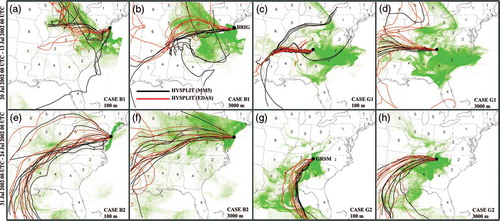
Figure 6. The spatial distribution of LSPDM particles (green dots) from the baseline simulations at 168 hr into the simulation for receptor depths of 100 and 3000 m for cases (a and b) B3, (e and f) B4, (c and d) G3, and (g and h) G4. HYSPLIT trajectories using MM5 (EDAS) inputs are shown as black (red) solid lines. Emission source region numbers and the receptor sites BRIG and GRSM are also shown in the figure.

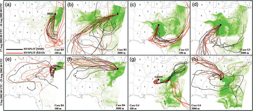
During weak vertical wind shear conditions and stronger southeasterly flow because of the southwestward ridge extension of the Bermuda High into the Gulf of Mexico (e.g., case 2), both LSPDM and HYSPLIT backward-trajectory analysis favor the receptor GRSM that is closer to the Gulf of Mexico. For case 3, the ridge extension is westward and more pronounced on the entire eastern maritime region because of the southern movement of the Bermuda High. Consequently, the success with respect to CMAQ simulations was similar for both receptors. However, during pronounced vertical wind shear conditions (e.g., case 4, Figures 6e–6h) the success of the HYSPLIT trajectory analysis highly depended on the selection of starting height for backward trajectories (Figure 3). In general, greater success can be obtained by including multiple particle backward trajectories from the deeper atmospheric layer compared with a few backward trajectories from selected heights.

Table 4 shows the regions that have the highest and second-highest contributions simulated by the CMAQ, LSPDM, and HYSPLIT models for each case. The LSPDM was better at identifying the first- and second-ranked source region contributions compared with HYSPLIT. The HYSPLIT trajectories largely underestimated the contributions of the nearby source regions (because of short residence time starting from the receptor sites, e.g., R1 for case B1) and overestimated the impacts of more distant regions (e.g., R7 for case B2). This can be attributed to differences in trajectory and stochastic dispersion methodologies.

Table 4. The first- (second-) highest contributing emission source regions estimated from the CMAQ SO₄ ²⁻ concentrations and from the average residence times of the backward trajectories

Case-ID (Receptor Location)	CMAQ (Shown in Table 2)	LSPDM (Baseline)		HYSPLIT (MM5)		HYSPLIT (EDAS)
		100 m	3000 m	100 m	≤3000 m	100 m	≤3000 m
B1 (BRIG)	R1 (R5)	R1 (R5)	R1 (R5)	R5 (R2)	R5 (R3)	R5 (R3)	R5 (R1)
B2 (BRIG)	R1 (R3)	R3 (R1)	R1 (R5)	R3 (R7)	R7 (R3)	R7 (R3)	R7 (R5)
B3 (BRIG)	R2 (R1)	R2 (R1)	R2 (R1)	R2 (R1)	R2 (R4)	R2 (R1)	R2 (R4)
B4 (BRIG)	R1 (R6)	R1 (R2)	R1 (R5)	R1 (R2)	R1 (R3)	R3 (R1)	R1 (R5)
G1 (GRSM)	R3 (R5)	R3 (R2)	R3 (R5)	R7 (R3)	R7 (R3)	R7 (R3)	R7 (R3)
G2 (GRSM)	R4 (R3)	R4 (R3)	R4 (R3)	R4 (R3)	R4 (R3)	R4 (R3)	R4 (R3)
G3 (GRSM)	R4 (R2)	R4 (R2)	R4 (R2)	R4 (R3)	R4 (R3)	R4 (R3)	R4 (R3)
G4 (GRSM)	R2 (R6)	R2 (R3)	R2 (R3)	R2 (R3)	R3 (R2)	R3 (R2)	R3 (R4)
Notes: Backward trajectories simulated by the LSPDM (receptor depths of 100 and 3000 m) and HYSPLIT (≤3000 m indicates HYSPLIT trajectory starting heights from and below 3000 m; i.e., 100, 500, 1000, 1500, and 3000 m). Exact agreement of LSPDM and HYSPLIT simulated source regions with CMAQ are shown in bold.

Regarding the CORs obtained from the normalized CMAQ SO₄ ²⁻ concentrations at the receptors versus normalized LSPDM and HYSPLIT residence times, except for case 2 (BRIG), the LSPDM results show similar correlations with CMAQ (0.7–0.99) for all heights. The results for case 2 indicate that the flow at the upper levels dominated most of the pollutant atmospheric transport. Consequently, inclusion of all depths from 100 to 3000 m improved the correlation for the LSPDM results. The overall COR for all LSPDM experiments ranged from 0.82 to 0.9 compared with H^M (H^E) CORs from 0.54 to 0.67 (0.48–0.61) (Figure 3). For example, in case G1 (Figures 5a–5d), the H^E trajectories significantly underestimate R1, R2, and R5 and overestimate R6 and R7.

There is a more uniform relationship between LSPDM-identified source region impact versus apportionment baseline impact simulated by the CMAQ model as compared with the H^M and H^E trajectories. The agreement is generally better for higher normalized concentrations. Average residence times from all heights above ground level improved the correlation of the normalized CMAQ concentrations versus normalized LSPDM residence times from 0.88 to 0.90. A slight improvement was found for the H^M (0.67) and H^E (0.61) CORs. As expected,34 the LSPDM with a smaller particle release volume, similar to the sensitivity tests described in the Modeling Approach section, yielded similar CORs. The LSPDM results with elevated starting points of particle releases at each receptor showed that the overall correlation dropped compared with the baseline and the smaller volume (Figure 3). This indicates the need to account for the spatial variations of the flow that are relevant to the atmospheric transport and uncertainties and errors in input wind fields.

The RMSE results are shown in Table 3. The LSPDM statistics obtained from the residence times averaged over all of the starting heights/depths in each region yielded uniform improvement. The statistical analysis confirmed that the LSPDM results generally produced half of the error compared with the backward-trajectory results. The values averaged over the volumes and heights slightly improved the RMSE for all cases. Although the backward-trajectory RMSEs vary for different cases, the lower-level particle releases appear to produce lower RMSEs than the higher-level releases. The backward trajectories starting from higher levels may exit the top boundary of the domain early because of overaccounting for subsidence.

Table 3. The RMSE obtained from the normalized results from the baseline LSPDM inverse simulations (receptor sizes: 1° × 1° × [100, 500, 1000, 1500, 3000 m]) and HYSPLIT backward trajectories for all cases with respect to the CMAQ results

Case ID	Comparison	≤100 m	≤500 m	≤1000 m	≤1500 m	≤3000 m	Mean^row
B1	CMAQ vs. LSPDM	0.09	0.08	0.12	0.13	0.12	0.11
	CMAQ vs. H^M (H^E)	0.33 (0.34)	0.34 (0.31)	0.33 (0.30)	0.33 (0.29)	0.35 (0.28)	0.33 (0.31)
B2	CMAQ vs. LSPDM	0.32	0.30	0.27	0.20	0.17	0.26
	CMAQ vs. H^M (H^E)	0.40 (0.40)	0.43 (0.43)	0.40 (0.44)	0.39 (0.45)	0.38 (0.45)	0.40 (0.43)
B3	CMAQ vs. LSPDM	0.07	0.05	0.06	0.09	0.25	0.13
	CMAQ vs. H^M (H^E)	0.12 (0.11)	0.15 (0.09)	0.27 (0.11)	0.30 (0.12)	0.33 (0.18)	0.25 (0.13)
B4	CMAQ vs. LSPDM	0.25	0.26	0.25	0.23	0.17	0.24
	CMAQ vs. H^M (H^E)	0.26 (0.39)	0.30 (0.42)	0.44 (0.42)	0.47 (0.47)	0.45 (0.43)	0.39 (0.43)
G1	CMAQ vs. LSPDM	0.14	0.14	0.14	0.14	0.14	0.14
	CMAQ vs. H^M (H^E)	0.37 (0.40)	0.38 (0.42)	0.38 (0.42)	0.38 (0.43)	0.38 (0.43)	0.38 (0.42)
G2	CMAQ vs. LSPDM	0.05	0.04	0.06	0.08	0.13	0.08
	CMAQ vs. H^M (H^E)	0.05 (0.03)	0.04 (0.04)	0.04 (0.07)	0.07 (0.12)	0.11 (0.18)	0.07 (0.10)
G3	CMAQ vs. LSPDM	0.06	0.06	0.06	0.07	0.09	0.07
	CMAQ vs. H^M (H^E)	0.11 (0.11)	0.11 (0.11)	0.12 (0.11)	0.12 (0.11)	0.11 (0.11)	0.11 (0.11)
G4	CMAQ vs. LSPDM	0.23	0.22	0.22	0.22	0.22	0.22
	CMAQ vs. H^M (H^E)	0.24 (0.38)	0.29 (0.38)	0.29 (0.38)	0.29 (0.39)	0.29 (0.36)	0.28 (0.38)
Mean^col	CMAQ vs. LSPDM	0.18	0.17	0.17	0.16	0.17	0.17
	CMAQ vs. H^M (H^E)	0.27 (0.31)	0.29 (0.32)	0.31 (0.32)	0.32 (0.33)	0.32 (0.33)	0.30 (0.32)
Notes: BRIG (GRSM) cases are indicated as B1–B4 (G1–G4). Mean^row = mean values by the row, Mean^col = mean values by the column; net result in bold.

The agreement between the reference simulations (CMAQ) and the LSPDM and backward-trajectory normalized residence times for each source region contribution is shown in Figure 7. Except for the R4 contributions, the LSPDM produced better agreement than the HYSPLIT results. H^M was more accurate than H^E over the entire range of source regions; however, it is somewhat surprising that the improvement of resolution from 80 km (H^E) to 12 km (H^M) yielded only modest improvement in the backward-trajectory comparisons with the reference simulations. It also confirms that the backward-trajectory calculations cannot accurately represent the impact of distant regions (R5–R7). The inverse modeling produced twice the number of normalized value pairs in agreement with the CMAQ-simulated results (123) compared with H^M (64) and H^E (60).

Figure 7. Histograms of the pairs of exact agreement for each emission source region R1–R7 between CMAQ and baseline LSPDM (left), CMAQ and H^M (center), and CMAQ and H^E (right).

One of the important questions is how accurately the inverse modeling techniques can rank contributions from different source regions. According to Figure 8, the highest contributing emission source regions were identified by the LSPDM (1° × 1° × depth volume) in 37 and for H^M (H^E) in 21 (16) of 40 cases. The second-highest contributing source regions were identified by the LSPDM in 21 and H^M (H^E) in 9 (11) of 40 cases. For the case of a single location as a starting point for inverse modeling and backward-trajectory analysis, the LSPDM shows similar success in identifying the first- and second-ranked regions of impact, whereas the results for H^M and H^E are noticeably lower. The latter results are mainly due to horizontal and vertical shear variations that are not taken into account for point location cases. The highest accuracy can be expected by using starting volumes compared with starting point locations.

Figure 8. Histograms of ranked pairs (from 280 pairs) in the simulations that used (a) a point source above the receptor and (b) a baseline area source centered at the receptor that are in exact agreement with the CMAQ-simulated first- and second-ranked emission source regions.

The work by Lowenthal et al.50 is an extension of a study to evaluate the ability of statistical- and trajectory-based receptor models to resolve regional contributions to PM_2.5 SO₄ ²⁻ using synthetic data at national parks in the eastern United States for the entire summer of 2002. Lowenthal et al.50 used the trajectory mass balance regression model to apportion SO₄ ²⁻ concentrations to regional-scale sources using HYSPLIT trajectories. The LSPDM was able to closely follow the CMAQ results in regions R1–R5 for both receptors, with some underestimation for R6 and overestimation for R7 (figure not shown). H^M and H^E show mixed results without any trends in success for all regions. Furthermore, the inclusion of all available HYSPLIT trajectories for all case periods in the verification only showed slight improvement in the correlations (Figure 4; shown as A2). Also, the HYSPLIT trajectories obtained from different horizontal grid resolutions (EDAS, 80 km; MM5, 12 km) did not significantly affect the correlations, which concurs with the HYSPLIT-based conclusions of other recent studies (Green,68 Pitchford et al.,69 Gebhart et al.,70 and Schichtel et al.71).

CONCLUSIONS

The LSPDM simulations and the HYSPLIT backward-trajectory analyses were able to determine source region contributions for many, but not all, cases of nearby and short-range transport. The LSPDM produced higher correlations (COR r = 0.89) compared with HYSPLIT using MM5 (r = 0.62) or EDAS (r = 0.55) wind fields. The LSPDM identified the primary emission source regions in 37 of 40 cases, whereas H^M (H^E) did so in 21 (16) of 40 cases. The second-ranked emission source regions were identified by the LSPDM in 21 of 40 cases and by H^M (H^E) in 9 (11) of 40 cases. Because LSPDM, CMAQ, and H^M use the same meteorological inputs from MM5, multiple particle trajectories in the same MM5 forcing environment reduce the uncertainty in the identification compared with those obtained from the single or very limited backward trajectories used in the HYSPLIT model calculations. The improvement of up to 45% in the CORs shows the direct benefit of using the LSPDM over the backward-trajectory analysis for identification of source regions. The RMSE analysis confirms that the LSPDM results generally produce half of the error compared with the backward-trajectory results.

In most of the cases considered in this study, H^E (HYSPLIT using EDAS inputs) trajectories showed more variability in the regional identification than H^M backward trajectories. In all considered cases, the trajectories tended to underestimate near-receptor sources because of the short residence time in the receptor area. On the other hand, the trajectories tended to overestimate the effects of distant sources because of intrinsic differences in trajectory and stochastic particle model methodologies.

HYSPLIT results were evaluated using different heights for the starting position of the backward trajectories (100, 500, 1000, 1500, and 3000 m). The results show better comparison with actual residence times using levels 1000 m and below than higher levels. The LSPDM was more accurate with a deeper layer of 3000 m. The contribution of the upper flows to the boundary layer winds can provide an important input for accurate estimates of the transport and dispersion.

Sensitivity experiments were conducted by changing the particle release volume at the receptor locations from 1° × 1° × depth to 0.05° × 0.05° × depth for all considered depths as well as considering the exact receptor location as a point source (Figure 3). The results of both tests yielded similar results compared with the baseline runs with 1° × 1° × depth for all considered depths. The baseline setup allowing for a wider range of horizontal flow shear still had the best overall correlation and the lowest RMSE (Table 3).

An additional test was conducted to examine the influence of turbulence and randomness on the Lagrangian stochastic particle results. Turbulence contribution was turned off and the same number of particle trajectories was selected as in the HYSPLIT computations for case 1. As expected, the COR between the CMAQ and LSPDM dropped to 0.52, whereas the full treatment of turbulence and randomness showed a COR of 0.91.

To reduce errors and uncertainties of the inverse Lagrangian modeling and backward-trajectory approaches because of the selection of a particular starting level within a large complex set of 3D winds, turbulence, and dispersion, an averaging of the results for all heights was computed as an ensemble average for the LSPDM results and HYSPLIT backward trajectories. These averaged values provided uniform improvement compared with all individual starting heights and volumes.

ACKNOWLEDGMENTS

This work was supported by a U.S. Environmental Protection Agency (EPA) Science to Achieve Results grant (EP-P21741/C10649) and an Electric Power Research Institute grant (C7750). The contents of this paper do not necessarily reflect the views and policies of EPA, nor does mention of trade names or commercial products constitute endorsement or recommendation for use.

REFERENCES

- Zannetti , P. 2005 . Air Quality Modeling: Theories, Methodologies, Computational Techniques, and Available Databases and Software—Volume II. Advanced Topics , Pittsburgh , PA : A&WMA .
- Watson , J.G. , Chow , J.C. and Fujita , E.M. 2001 . Review of Volatile Organic Compound Source Apportionment by Chemical Mass Balance . Atmos. Environ. , 35 : 1567 – 1584 .
- Watson , J.G. , Zhu , T. , Chow , J.C. , Engelbrecht , J.P. , Fujita , E.M. and Wilson , W.E. 2002 . Receptor Modeling Application Framework for Particle Source Apportionment . Chemosphere , 49 : 1093 – 1136 .
- Watson , J.G. , Chen , L.-W.A. , Chow , J.C. , Lowenthal , D.H. and Doraiswamy , P. 2008 . Source Apportionment: Findings from the U.S. Supersite Program . Journal of the Air & Waste Management Association , 58 : 265 – 288 . doi: 10.3155/1047-3289.58.2.265
- Guidance on the Use of Models and Other Analyses for Demonstrating Attainment of Air Quality Goals for Ozone, PM2.5, and Regional Haze; EPA-454/B-07-002; U.S. Environmental Protection Agency: Research Triangle Park, NC, 2007 http://www.epa.gov/ttn/scram/guidance/guide/final-03-pm-rh-guidance.pdf (http://www.epa.gov/ttn/scram/guidance/guide/final-03-pm-rh-guidance.pdf) (Accessed: 2011 ).
- Ashbaugh , L.L. 1983 . A Statistical Trajectory Technique for Determining Air Pollution Source Regions . J. Air Poll. Control Assoc. , 33 : 1096 – 1098 .
- Rodean , H. 1996 . Stochastic Lagrangian Models of Turbulent Diffusion . Meteorol. Mono. , 26 : 4740 – 4750 .
- Zannetti , P. and Zannetti , P. 1992 . Environmental Modeling , Edited by: Melli , P. Southampton , , United Kingdom : Computational Mechanics Publications .
- Flesch , T.K. , Wilson , J.D. and Yee , E. 1995 . Backward-Time Lagrangian Stochastic Dispersion Models and Their Application to Estimate Gaseous Emissions . J. Appl. Meteorol. , 34 : 1320 – 1332 .
- Uliasz , M. and Pielke , R.A. 1990 . Computer Techniques in Environmental Studies III , Edited by: Zannetti , P. 57 – 68 . Berlin , , Germany : Springer-Verlag .
- Flesch , T.K. and Wilson , J.D. 2005 . Micrometeorology in Agricultural Systems , Edited by: Hartfield , J.L. and Baker , J.M. 513 – 531 . Madison , WI : American Society of Agronomy .
- Giering , R. 1999 . Inverse Methods in Global Biogeochemical Cycles , 33 – 48 . Washington , DC : American Geophysical Union .
- Hourdin , F. and Issartel , J.P. 2000 . Subsurface Nuclear Tests Monitoring through the CTBT Xenon Network . Geophys. Res. Lett. , 27 : 2245 – 2248 .
- Robertson , L. and Persson , C. 1992 . Air Pollution Modeling and Its Applications , Edited by: van Dop , H. and Kallos , G. 365 – 373 . New York : Plenum .
- Uliasz , M. and Pielke , R.A. 1992 . Air Pollution Modeling and Its Applications , Edited by: van Doop , H. 171 – 178 . New York : Plenum .
- Eliassen , A. 1980 . A Review of Long-Range Transport Modeling . J. Appl. Meteorol. , 19 : 231 – 240 .
- Fisher , B.E.A. 1983 . A Review of the Processes and Models of Long-Range Transport of Air Pollutants . Atmos. Environ. , 17 : 1865 – 1880 .
- Holmes , N.S. and Morawska , L. 2006 . A Review of Dispersion Modelling and Its Application to the Dispersion of Particles: an Overview of Different Dispersion Models Available . Atmos. Environ. , 40 : 5902 – 5928 .
- Stohl , A. 1998 . Computation, Accuracy and Applications of Trajectories—a Review and Bibliography . Atmos. Environ. , 32 : 947 – 966 .
- Wilson , J.D. 1996 . Review of Lagrangian Stochastic Models for Trajectories in the Turbulent Atmosphere . Bound. Layer Meteorol. , 78 : 191 – 210 .
- Cao , J.J. , Lee , S. , Zheng , X. , Ho , K. , Zhang , X. , Guo , H. , Chow , J.C. and Wang , H. 2003 . Characterization of Dust Storms to Hong Kong in April 1998 . Water Air Soil Pollut. , 3 : 213 – 229 .
- Chen , L.-W.A. , Doddridge , B.G. , Dickerson , R.R. , Chow , J.C. and Henry , R.C. 2002 . Origins of Fine Aerosol Mass in the Baltimore-Washington Corridor: Implications from Observation, Factor Analysis, and Ensemble Air Parcel Back Trajectories . Atmos. Environ. , 36 : 4541 – 4554 .
- Gebhart , K.A. , Schichtel , B.A. and Barna , M.G. 2005 . Directional Biases in Back Trajectories Due to Model and Input Data . Journal of the Air & Waste Management Association , 55 : 1649 – 1662 .
- Kang , C.M. , Kang , B.W. and Lee , H.S. 2006 . Source Identification and Trends in Concentrations of Gaseous and Fine Particulate Principal Species in Seoul, South Korea . Journal of the Air & Waste Management Association , 56 : 911 – 921 .
- Kavouras , I.G. , Etyemezian , V. and DuBois , D.W. 2009 . Development of a Geospatial Screening Tool to Identify Source Areas of Windblown Dust . Environ. Model. Software , 24 : 1003 – 1011 .
- Louie , P.K.K. , Watson , J.G. , Chow , J.C. , Chen , L.-W.A. , Sin , D.W.M. and Lau , A.K.H. 2005 . Seasonal Characteristics and Regional Transport of PM2.5 in Hong Kong . Atmos. Environ. , 39 : 1695 – 1710 .
- Occhipinti , C. , Aneja , V.P. , Showers , W. and Niyogi , D. 2008 . Back-Trajectory Analysis and Source-Receptor Relationships: Particulate Matter and Nitrogen Isotopic Composition in Rainwater . Journal of the Air & Waste Management Association , 58 : 1215 – 1222 . doi: 10.3155/1047-3289.58.9.1215
- Sprovieri , F. and Pirrone , N. 2008 . Particle Size Distributions and Elemental Composition of Atmospheric Particulate Matter in Southern Italy . Journal of the Air & Waste Management Association , 58 : 797 – 805 . doi: 10.3155/1047-3289.58.6.797
- Xu , J. , DuBois , D.W. , Pitchford , M.L. , Green , M.C. and Etyemezian , V. 2006 . Attribution of Sulfate Aerosols in Federal Class I Areas of the Western United States Based on Trajectory Regression Analysis . Atmos. Environ. , 40 : 3433 – 3447 .
- Zhou , L. , Hopke , P.K. and Zhao , W.X. 2009 . Source Apportionment of Airborne Particulate Matter for the Speciation Trends Network Site in Cleveland, OH . Journal of the Air & Waste Management Association , 59 : 321 – 331 . doi: 10.3155/1047-3289.59.3.321
- Lin , J.C. , Gerbig , C. , Wofsy , S.C. , Andrews , A.E. , Daube , B.C. , Davis , K.J. and Grainger , C.A. 2003 . A Near-Field Tool for Simulating the Upstream Influence of Atmospheric Observations: The Stochastic Time-Inverted Lagrangian Transport (STILT) Model . J. Geophys. Res.-Atmos. , 108 doi: 10.1029/2002JD003161
- Seibert , P. 2001 . Air Pollution Modeling and Applications , Edited by: Schiermeiser , F. and Gryning , E. New York : Plenum .
- Thomson , D.J. 1987 . Criteria for the Selection of Stochastic Models of Particle Trajectories in Turbulent Flows . J. Fluid Mechan. , 180 : 529 – 556 .
- Seibert , P. and Frank , A. 2004 . Source-Receptor Matrix Calculation with a Lagrangian Particle Dispersion Model in Backward Mode . Atmos. Chem. Phys. , 4 : 51 – 63 .
- Chow , J.C. , Engelbrecht , J.P. , Watson , J.G. , Wilson , W.E. , Frank , N.H. and Zhu , T. 2002 . Designing Monitoring Networks to Represent Outdoor Human Exposure . Chemosphere , 49 : 961 – 978 .
- Huang , A.H. and Head , S.J. 1978 . Estimation of Fugitive Hydrocarbon Emissions from an Oil Refinery by Inverse Modeling , Washington , DC : U.S. Environmental Protection Agency .
- Sattler , M. and Devanathan , S. 2007 . Which Meteorological Conditions Produce Worst-Case Odors from Area Sources? . Journal of the Air & Waste Management Association , 57 : 1296 – 1306 . doi: 10.3155/1047-3289.57.11.1296
- Gao , Z.L. , Desjardins , R.L. , van Haarlem , R.P. and Flesch , T.K. 2008 . Estimating Gas Emissions from Multiple Sources Using a Backward Lagrangian Stochastic Model . Journal of the Air & Waste Management Association , 58 : 1415 – 1421 . doi: 10.3155/1047–3289.58.11.1415
- Flesch , T.K. , Harper , L.A. , Desjardins , R.L. , Gao , Z.L. and Crenna , B.P. 2009 . Multi-Source Emission Determination Using an Inverse Dispersion Technique . Bound. Layer Meteorol. , 132 : 11 – 30 .
- Zhang , S. , Penner , J.E. and Torres , O. 2005 . Inverse Modeling of Biomass Burning Emissions Using Total Ozone Mapping Spectrometer Aerosol Index for 1997 . J. Geophys. Res. Atmos. , 110 doi: 10.1029/2004JD005738
- Chen , Y.H. and Prinn , R.G. 2006 . Estimation of Atmospheric Methane Emissions between 1996 and 2001 Using a Three-Dimensional Global Chemical Transport Model . J. Geophys. Res. , 111 doi: 10.1029/2005JD006058
- Stohl , A. , Seibert , P. , Arduini , J. , Eckhardt , S. , Fraser , P. , Greally , B.R. , Lunder , C. , Maione , M. , Muhle , J. , O'Doherty , S. , Prinn , R.G. , Reimann , S. , Saito , T. , Schmidbauer , N. , Simmonds , P.G. , Vollmer , M.K. , Weiss , R.F. and Yokouchi , Y. 2009 . An Analytical Inversion Method for Determining Regional and Global Emissions of Greenhouse Gases: Sensitivity Studies and Application to Halocarbons . Atmos. Chem. Phys. , 9 : 1597 – 1620 .
- HYSPLIT—HYbrid Single Particle Lagrangian Integrated Trajectory Model; National Oceanic and Atmospheric Administration; Air Resources Laboratory: Silver Springs, MD, 2009 http://ready.arl.noaa.gov/HYSPLIT.php (http://ready.arl.noaa.gov/HYSPLIT.php) (Accessed: 2011 ).
- Koracin , D. , Panorska , A. , Isakov , V. , Touma , J. S. and Swall , J. 2007 . A Statistical Approach for Estimating Uncertainty in Dispersion Modeling: an Example of Application in Southwestern USA . Atmos. Environ. , 41 : 617 – 628 .
- Stohl , A. , Haimberger , L. , Scheele , M.P. and Wernli , H. 2001 . An Intercomparison of Results from Three Trajectory Models . Meteorol. Appl. , 8 : 127 – 135 .
- VIEWS Visibility Information Exchange Web System; Colorado State University: Fort Collins, CO, 2010 http://vista.cira.colostate.edu/views (http://vista.cira.colostate.edu/views) (Accessed: 2011 ).
- Byun , D. and Schere , K.L. 2006 . Review of the Governing Equations, Computational Algorithms, and Other Components of the Models-3 Community Multiscale Air Quality (CMAQ) Modeling System . Appl. Mechan. Rev. , 59 : 51 – 77 .
- Wheeler , N. , Craig , K. and Reid , S. Simulating IMPROVE-Like Data for Use in Evaluating Receptor Models . STI-906046.01-3179 . 2007 . Sonoma Technology: Petaluma, CA
- Chen , L.-W.A. , Lowenthal , D.H. , Watson , J.G. , Koracin , D. , Kumar , N. , Knipping , E.M. , Wheeler , N. , Craig , K. and Reid , S. 2010 . Toward Effective Source Apportionment Using Positive Matrix Factorization: Experiments with Simulated PM2.5 Data . Journal of the Air & Waste Management Association , 60 : 43 – 54 . doi: 10.3155/1047-3289.60.1.43
- Lowenthal , D.H. , Watson , J.G. , Koracin , D. , Chen , L.-W.A. , DuBois , D. , Vellore , R. , Kumar , N. , Knipping , E.M. , Wheeler , N. , Craig , K. and Reid , S. 2010 . Evaluation of Regional Scale Receptor Modeling . Journal of the Air & Waste Management Association , 60 : 26 – 42 . doi: 10.3155/1047-3289.60.1.26
- Chow , J.C. , Watson , J.G. and Chen , L.-W.A. 2006 . Contemporary Inorganic and Organic Speciated Particulate Matter Source Profiles for Geological Material, Motor Vehicles, Vegetative Burning, Industrial Boilers, and Residential Cooking , Springfield , VA : Prepared by Desert Research Institute, Reno, NV, for Pechan and Associates .
- Grell , G.A. , Dudhia , J. and Stauffer , D.R. 1994 . A Description of the Fifth-Generation Penn State/NCAR Mesoscale Model (MM5) , Boulder , CO : National Center for Atmospheric Research (NCAR) Technical Note NCAR/TN-398+STR; NCAR .
- Black , T.L. 1994 . The New NMC Mesoscale Eta Model: Description and Forecast Examples . Weather Forecast. , 9 : 265 – 278 .
- Rolph , G.D. NCEP Model Output—EDAS Archive . TD-6141 . 2002 . National Oceanic and Atmospheric Administration; Air Resources Laboratory: Silver Spring, MD
- Pielke , R.A. 1984 . Mesoscale Meteorological Modeling , New York : Academic .
- Rodean , H.C. 1996 . Stochastic Lagrangian Models of Turbulent Diffusion , Boston , MA : American Meteorological Society .
- Hanna , S.R. 1982 . Atmospheric Turbulence and Air Pollution Modeling , Edited by: Nieuwstadt , F.T.M. and Van Dop , H. Dordrecht , , The Netherlands : Kluwer .
- Gifford , F.A. 1995 . Some Recent Long-Range Diffusion Experiments . J. Appl. Meterol. , 34 : 1727 – 1730 .
- Legg , B.J. and Raupach , M.R. 1982 . Markov Chain Simulation of Particle Dispersion in Inhomogenous Flows: the Mean Drift Velocity Induced by a Gradient in Eulerian Velocity Variance . Bound. Layer Meteorol. , 24 : 3 – 13 .
- Donaldson , C.P. 1973 . “ Three-Dimensional Modeling of the Planetary Boundary Layer ” . In Proceedings of a Workshop on Micrometeorology , Edited by: Haugen , A. Boston , MA : American Meteorological Society .
- Mellor , G.L. and Yamada , T. 1974 . A Hierarchy of Turbulence Closure Models for Planetary Boundary Layers . J. Atmos. Sci. , 31 : 1791 – 1806 .
- Andrén , A. 1990 . Evaluation of a Turbulence Closure Scheme Suitable for Air-Pollution Applications . J. Appl Meterol. , 29 : 224 – 239 .
- Luria , M. , Tanner , R.L. , Valente , R.J. , Bairai , S.T. , Koracin , D. and Gertler , A. W. 2005 . Local and Transported Pollution over San Diego, California . Atmos. Environ. , 39 : 6765 – 6776 .
- Weinroth , E. , Stockwell , W.R. , Koracin , D. , Kahyaoglu-Koracin , J. , Luria , M. , McCord , T. , Podnar , D. and Gertler , A.W. 2008 . A Hybrid Model for Ozone Forecasting . Atmos. Environ. , 42 : 7002 – 7012 .
- Mellor , G.L. and Yamada , T. 1982 . Development of a Turbulence Closure Model for Geophysical Fluid Problems . Rev. Geophys. , 20 : 851 – 875 .
- Hidy , G.M. 1994 . Atmospheric Sulfur and Nitrogen Oxides. Eastern North American Source-Receptor Relationships , San Diego , CA : Academic .
- Wang, J.X.L.; Angell, J.K. Air Stagnation Climatology for the United States (1949–1998); National Oceanic and Atmospheric Administration: Silver Spring, MD, 1999 http://www.arl.noaa.gov/documents/reports/atlas.pdf (http://www.arl.noaa.gov/documents/reports/atlas.pdf) (Accessed: 2011 ).
- Green , M. , Pitchford , M. and Tomback , I. A Summary of Findings from the Big Bend Regional Aerosol and Visibility Observational (BRAVO) Study . Presented at the 96th Annual A&WMA Conference . San Diego , CA . Pittsburgh , PA : A&WMA .
- Pitchford, M.L.; Tombach, I.; Barna, M.; Gebhart, K.A.; Green, M.C.; Knipping, E.; Kumar, N.; Malm, W.C.; Pun, B.; Schichtel, B.A.; Seigneur, C. Big Bend Regional Aerosol and Visibility Observational Study; Final Report; 2004 http://vista.cira.colostate.edu/improve/studies/BRAVO/reports/FinalReport/bravofinalreport.htm (http://vista.cira.colostate.edu/improve/studies/BRAVO/reports/FinalReport/bravofinalreport.htm) (Accessed: 2011 ).
- Gebhart , K.A. , Schichtel , B.A. and Barna , M.G. 2005 . Directional Biases in Back Trajectories Caused by Model and Input Data . Journal of the Air & Waste Management Association , 55 : 1649 – 1662 .
- Schichtel , B.A. , Gebhart , K.A. , Barna , M.G. and Malm , W.C. 2006 . Association of Airmass Transport Patterns and Particulate Sulfur Concentrations at Big Bend National Park, Texas . Atmos. Environ. , 40 : 992 – 1006 .
- Watson , J.G. 2002 . Visibility: Science and Regulation—2002 Critical Review . Journal of the Air & Waste Management Association , 52 : 628 – 713 .