Spatial modelling of wetness for the Antarctic Dry Valleys

Abstract

This paper describes a method used to model relative wetness for part of the Antarctic Dry Valleys using Geographic Information Systems (GIS) and remote sensing. The model produces a relative index of liquid water availability using variables that influence the volume and distribution of water. Remote sensing using Moderate Resolution Imaging Spectroradiometer (MODIS) images collected over four years is used to calculate an average index of snow cover and this is combined with other water sources such as glaciers and lakes. This water source model is then used to weight a hydrological flow accumulation model that uses slope derived from Light Detection and Ranging (LIDAR) elevation data. The resulting wetness index is validated using three-dimensional visualization and a comparison with a high-resolution Advanced Land Observing Satellite image that shows drainage channels. This research demonstrates that it is possible to produce a wetness model of Antarctica using data that are becoming widely available.

• GIS
• water
• Antarctica
• remote sensing.

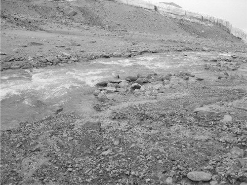
In Antarctica the severely limited availability of liquid water is a significant factor governing the distribution of terrestrial life. Antarctica has a vast store of ice with an average thickness of over 2 km covering over 95% of the continent (Peck et al. 2006), but very little of this water is available to life since it is not in liquid form. Antarctica's cold climate means humidity is extremely low, precipitation is scarce and the combined effects of cold and wind create a high rate of sublimation. For these reasons, Antarctica is often described as the driest continent on Earth. Water is the essential ingredient of all terrestrial ecosystem functions including chemical and physical change, nutrient transportation and leaching and biological activity and interactions (Campbell et al. 1997). The freezing and melting of water can be seen as a binary switch, turning off and on biological activity (Kennedy 19931999; Fountain et al. 1999). For short periods of the summer (December and January) there can be large amounts of liquid water available as lakes, pools and streams. Even in the southern Dry Valleys, the runoff of water can be significant in the summer, with reasonably fast flowing streams forming (Fig. 1).

Fig. 1.  Stream flow in Garwood Valley, southern Victoria Land, Antarctica, January 2009. Garwood Glacier is in the background.

The aim of this paper is to demonstrate a method to model the relative distribution of available water. The intention is that this model can feed into other research projects that are attempting to model the distribution of species in Antarctica. The research presented in this paper is part of a larger project that aims to improve understanding of the complex relationship between the different terrestrial life forms in Antarctica including bacteria, soil microbes, microarthropods, algae, lichens and moss.

The isolation and cold climate makes it difficult to obtain abiotic data for Antarctic but this has changed recently with increased availability of remotely sensed data, which includes a range of satellite data of various spatial, spectral and temporal resolutions. It also includes data collected by sensors located on aircraft including height detecting devices such as Light Detection and Ranging (LIDAR) technology and stereography that have produced elevation surfaces (digital elevation models [DEM]). The use of remote sensing to model abiotic character has advantages because it reduces the need for field surveys and associated logistical requirements that are greatly increased due to Antarctica's isolation and the extreme environment. Fieldwork in Antarctica also has high risks of negative environmental impacts because of the relatively pristine environment and the fact that small amounts of contamination can significantly alter the environments and reduce the potential for future research.

The Dry Valleys

The Dry Valleys are an important research site because they are the continent's largest continuous expanse of ice-free ground—approximately 6000 km2 (Hemmings 2001). Terrestrial life on the Antarctic continent exists in the relatively limited ice-free areas and approximately half of this ice-free ground occurs within the Ross Sea region, particularly in the McMurdo Dry Valleys of southern Victoria Land.

The Dry Valleys were formed by glaciers gouging deep valleys in a generally east–west orientation. These valleys were cut off from the flow of glaciers and ice from Antarctica's interior by the uplift of the Transantarctic Mountains. They remain ice-free through ablation of snow and ice, which exceeds any accumulation (Horowitz et al. 1972; Friedmann 1982; Fountain et al. 1999; Fitzsimons et al. 2001; Hopkins et al. 2006).

The Dry Valleys of Antarctica contain alpine, piedmont and terminal glaciers, lakes mostly under permanent ice cover, bare soils and stream channels (Gooseff et al. 2003). Their mean annual air temperature is –20 to –25°C (Doran et al. 2002) and in summer the temperature rarely rises more than 0°C. However, the ground temperature may reach higher than 15°C for short periods during the day (Horowitz et al. 1972). For two to three months during the austral summer there is continual daylight and during the winter months there is continual darkness with valley floor temperatures falling as low as –40°C (Fountain et al. 1999). The cold temperatures vastly decrease water vapour content in the atmosphere and precipitation is scant (Horowitz et al. 1972), therefore qualifying the valleys as cold deserts (Peck et al. 2006). In the Dry Valley region the mean precipitation is limited to around 10 cm per year in the form of snow (Fountain et al. 1999). This aridity is enhanced in the Dry Valleys by the dry katabatic (downslope) winds off the Antarctic plateau increasing ablation and creating true desert conditions (Friedmann 1982). Ventifacts and wind-drifted pebble ridges are created by these constant winds and, due to the low humidity, the snow often sublimes without any visible wetting of the ground (Horowitz et al. 1972).

According to Gooseff et al., “The hydrologic system of the coastal McMurdo Dry Valleys, Antarctica, is defined by snow accumulation, glacier melt, stream flow and retention in closed-basin, ice-covered lakes” (2006: 1). This hydrologic system will vary between different valleys in the Dry Valley region depending on variation in snow fall, the number of glaciers flowing into the valleys and the topographical surface of the valleys.

Study area

The study area of this project is three valleys in the Denton Hills area of southern Victoria Land, the Garwood, Marshall and Miers valleys, and has a total area of approximately 300 km2 (Fig. 2). These valleys are smaller than the large Dry Valleys further north, yet the diversity of these valleys is representative of the Antarctic Dry Valley environment. The elevation of the study area ranges from sea level to approximately 1300 m.

Fig. 2.  Garwood, Marshall and Miers valleys, southern Victoria Land, Antarctica. Map, by Glen Stichbury, is based on data from the US Geological Survey's 1:250,000-scale topographic map (1986) and the Antarctic Digital Database.

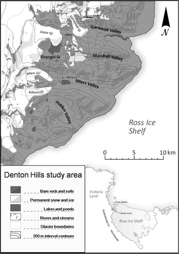
The study area contains many glaciers and as a result is likely to be wetter than some of the northern Dry Valleys such as the Baltham, McKevey and Wright valleys that have fewer glaciers feeding into them, relative to their sizes. The study area does not have large closed basins that prevent water flow, unlike the northern Dry Valleys. All three valleys in the study area have streams in the summer months that flow to the Ross Sea.

Wetness modelling

The wetness model brings together a combination of models that individually have been used and tested extensively, but together become an original and relatively simple method for representing a wetness surface for the Antarctic environment. The core of the model is the compound topographic index (CTI), also referred to as a compound terrain index or topographic wetness index. This is a steady-state wetness index that is based on a function of both slope and upstream contributing area (Moore et al. 1993; Yang et al. 2005).

Using a DEM, a CTI will compute the likely wetness of a given unit within the watershed by calculating the amount of water flowing into that unit. The value assigned is affected by slope. Where slope is steep, water drains quickly but where areas are flat, water accumulates especially if there is a large watershed flowing into this flat area. A CTI requires a DEM and can be calculated relatively easily using Geographic Information Systems (GIS). Detail on the source of the DEM used and the individual steps for calculating the CTI are described in a later section.

The standard CTI assumes that water is evenly distributed throughout the area of interest and flows overland according to the steepest slope. This would be the case when you have even rainfall over a catchment. However, in Antarctica rainfall is unlikely and the main sources of water are melting snow, glaciers and lakes, which are unevenly distributed. The CTI can be modified to include this uneven distribution of water by using a weighted grid to represent the irregular distribution of water sources. The CTI used in this research represents an average index of wetness over several seasons given the mean snow cover and locations of glaciers and lakes.

The wetness index therefore requires the input of several sub-models of water sources. Glaciers and lakes are relatively simple to model since their locations are static and can be easily identified from satellite images and digitized or classified using image analysis. Modelling the distribution of snow is more difficult because it fluctuates with seasons and by year. The following two sections describe the methods for calculating a snow index and the flow path algorithm. These are then integrated with the CTI.

Mean snow cover index

Snow cover can be modelled using complex algorithms that consider precipitation and the effects of wind and terrain. However, a much simpler method, which was used in this research, is to observe snow cover distribution using the increasingly available number of satellite images. Observations of snow distribution over an extended time can be combined to produce a probability model of snow distribution.

The Moderate Resolution Imaging Spectroradiometer (MODIS) sensors aboard the Terra and Aqua satellites of the National Aeronautics and Space Administration (NASA) provide frequent images of the study area (up to six passes a day due to their polar orbits) and can be downloaded freely from the MODIS Rapid Response System website (http://rapidfire.sci.gsfc.nasa.gov/). These provide a subset of true-colour (MODIS bands 1: 620–670 nm, 3: 459–479 nm and 4: 545–565 nm) and shortwave infrared images (SWIR; MODIS bands 5: 1230 nm, 6: 1652 nm and 7: 2105 nm). The spatial resolution of MODIS images varies with the bands: bands 1–2 are 250 m, 3–7 are 500 m and 8–36 are 1000 m.

The available images begin in November 2004 and continue to be updated daily. However, as MODIS is a passive system, images of the study area are only available from early September to early April, coinciding with the austral summer. For the remaining months, the study area is under constant darkness so data cannot be captured. This period of no data capture does not pose a problem in this project as any liquid water only exists in the Dry Valleys during the summer when the data are being captured. For this study, cloud-free images were downloaded from the Terra mission only as the Aqua satellite has a malfunctioning band 6. In total, 167 images were used from the four available summer seasons.

A technique known as the normalized difference snow index (NDSI) is available for identifying snow and is based on the relative magnitude between visible and shortwave infrared reflectance of snow (Hall et al. 2001). The MODIS instrument's version of the NDSI is:where r4 is the reflectance in band 4 and r6 is the reflectance in band 6 (Hall et al. 2001.

The MODIS NDSI data (MOD10A1.5) for the study area were obtained from the Earth Observing System data pool at the National Snow and Ice Data Center (http://nsidc.org/index.html). This data set contains snow cover data based on the MODIS NDSI algorithm and automatic cloud detection. The data is obtained in 1200 km×1200 km tiles at a 500-m resolution. These tiles provide excellent information for use in large-scale regional snow cover studies but were unsuitable for this study. There were often no data or clouds reported for sections of the study area when this was not the case. This may be because the study area was located near the periphery of the tiles and there would have been complications due to the angle from the instrument to the study area.

For this study an unsupervised classification method was used to distinguish snow from rock. Unsupervised classification uses a clustering technique to assign pixels to classes (Rees 1999). The 167 images were classified using the Isodata clustering algorithm in the ArcGIS software program. Each image was cloud-free for the study area, based on manual selection, which meant that the process was not complicated by cloud-masking techniques. The signature file used for the unsupervised classification was identified from an image captured on 18 September 2005. This image was selected, after investigating a range of images, because the sun is low and the effects of different lighting are exaggerated. Since 167 images required classification, this process was automated and this was made easier by using just the one signature file. A limitation with snow detection is the difficulty of identifying snow in the dark shadows, which are generally on the south-facing slopes.

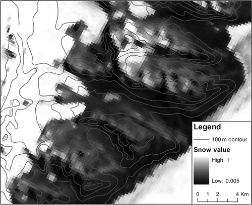
From the classification of 167 images, the proportion each pixel was classified as snow was calculated. This resulted in a grid (Fig. 3) showing the probability of snow cover based on the average of four summer seasons: (0) indicated permanently bare rock and (1) permanent snow and ice cover. This output is based on empirical data and provides a very good indication of the distribution of ice and snow. As expected, the permanent glaciers and frozen lakes have a high value. It is apparent from this analysis that there is more snow in the higher elevations and on the northern slopes. The latter could be because the south-facing slopes in the study area are generally steeper than the north-facing slopes. Also, as previously mentioned, the south-facing slopes are more likely to be in shadow, making it difficult to detect snow.

Fig. 3.  Mean snow cover index.

Flow path accumulation

In the austral summer of 2001/02, NASA's Airborne Topographic Mapper (ATM) system was used to collect almost 4000 km² of elevation data at several sites in the McMurdo Sound region. The ATM system uses LIDAR technology from an aircraft platform to produce a highly detailed surface topography (Wilson & Csathó 2007). The Denton Hills was an area captured. The average laser spot density was at least one point per 6 m² and the overall vertical accuracy of the operation was identified to be 0.2 m (Wilson & Csathó 2007). This data set is a huge improvement compared to the only alternative data set—the 200-m contours from the Antarctic Digital Database (Thomson & Cooper 1993).

Various algorithms have been devised for the calculation of water-flow paths for wetness indices, stream networking and other watershed analysis functions including D8 (O'Callaghan & Mark 1984), Rho8 (Fairfield & Leymarie 1991), Multiple Flow (Quinn et al. 1991), DEMON (Costa-Cabral & Burges 1994) and D-Infinity (Tarboton 1997). These different approaches to calculating the direction of water flow, and thus upslope contributing area, all follow the principle that gravity causes water to flow overland in a downslope direction (Wilson & Gallant 2000). The approach to flow-path calculation used in this study was the D-Infinity (D-Inf) algorithm (Tarboton 1997). D-Inf divides each 3×3 cell window (centred on the cell of interest) into eight triangular facets using the cell centres as vertices. From these facets, slope, flow direction and magnitude are calculated, flowing either down one of the 45° angles between cells or proportionally into multiple downhill cells (Tarboton 19972003).

Contributing area calculated for each grid cell is taken as its own contribution plus the upslope cells that drain into that cell (Tarboton 2003). With a standard upslope contributing area calculation, each cell is counted using a value of one. Each cell value is then calculated recursively to its value plus that of the neighbouring cell(s) at the steepest upslope angle. The mean snow cover index (Fig. 3) is used as a weighted grid representing heterogeneous water availability and it assumes that some of the snow will melt rather than sublime. The recursive procedure sums the weighted cell value, which is a proportion of one. The flow accumulation is therefore based on the potential availability of melt water that flows into each cell.

Weighted CTI

The final step in the process of creating the model is the calculation of the CTI. This is done through the use of an Arc Macro Language script called Compound Topographic Index (Evans 2003) obtained from Esri's (Redlands, CA, USA) ArcScripts website (http://arcscripts.esri.com). This script was run in ArcInfo Workstation using the GRID extension. The inputs used in running this script were a 10-m resolution DEM of the study area and the optional weighted flow accumulation grid calculated above. The 10-m resolution DEM was used because the flow paths are computationally intensive and 10-m resolution was the best compromise between detail and functionality. Wilson & Gallant (2000) have also confirmed that the differences in results with finer resolutions are minimal.

The overall formula for the CTI can be shown as:where a=area value calculated as (flow accumulation)×(cell size) and β is the slope expressed in radians (Evans 2003). The flow accumulation value is calculated from the weighted contributing area grid and the cell size is 10 m. A linear cell dimension is used for cell size rather than the actual pixel area.

Results and validation

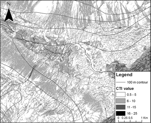
Fig. 4 shows the final wetness model, which is an index of the predicted spatial availability of liquid water, given the spatial distribution of water sources and the effects of gravity and topography. Fig. 5 shows an enlargement of the lower Miers Valley. Although moraine dominates much of this area, this image clearly shows the drainage channel of the Miers stream and the minor drainage channels on the sides of the valley. For the whole study area, the index varies from 23.8 at its wettest to 0.5 at its driest. Lakes Miers and Budda have CTI values from 10 to 15, while the higher CTI values (>20) are found in the lower stream beds. The highest values are found at the mouth of the Garwood and Miers streams. The lower values are found on the steep slopes, which for this study area also tend to have southern aspect. The slopes with southern aspect may have exaggerated dryness because of the difficulty in identifying snow from the shadows in the MODIS images. The mean and median values for the entire study area are 6.8 and 12.1, respectively.

Fig. 4.  Final wetness model showing the compound topographic index (CTI).

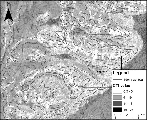
Fig. 5.  Enlargement of the Lower Miers Valley showing the compound topographic index (CTI) in the final wetness model.

Although observations in the field support the model, qualitative GIS visualization techniques were used for validating the method. Quantitatively validating the method using systematically collected wetness measurements in the field is not practical given the isolated environment and the temporal and spatial variability of available water. Instead, qualitative assessment was used based on two different visualization techniques: three-dimensional visualization and an overlay comparison with a high-resolution satellite image.

ArcGlobe software was used to construct a three-dimensional perspective view of the study area, which allowed viewing of the underlying terrain and the wetness model. This software enabled the wetness model to be compared with the topography and assessed as to whether the model fitted with expected drainage patterns. The three-dimensional view, using a 4-m-resolution DEM, clearly shows ridges and gullies and micro-relief features. The wetness index was qualitatively assessed to ensure that the drainage associated with these features conformed to what is expected. Some caution is required with this assessment because the Dry Valleys contains many relict stream channels, preserved due to the extremely slow geomorphic processes in the valleys and the lack of water and vegetation. Therefore, the existence of a stream channel on the landscape does not necessarily mean that liquid water will be found in that location under our modern climate.

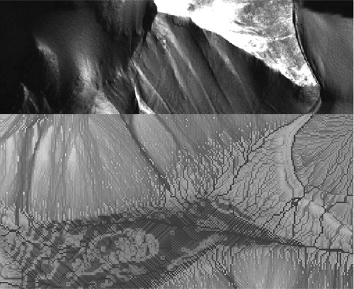
The wetness index was also overlaid on a high-resolution (<4 m²) Advanced Land Observing Satellite (ALOS) panchromatic image captured on 30 November 2007 (Fig. 6). This high-resolution image shows rills and gullies on the valley sides where meltwater flows. Also visible are streams on the valley floors, alluvial fans, lakes and ponds. Figure 6 shows how the wetness index and ALOS image can be overlaid and “swiped” to show the underlying image using ArcMap's Effects toolbar. By clicking and dragging on the overlaying image layer, the data underneath are revealed. From this it can be seen that the drainage patterns and ponds are aligned, showing higher water accumulation in drainage streams visible in the ALOS image. Values are increasing at lowering elevations and increased stream orders. Based on the visual comparison with drainage patterns shown in the ALOS image and the three-dimensional views, the weighted CTI index appears to provide a realistic model of wetness.

Fig. 6.  The swipe tool shows alignment of drainage channels between the wetness model and Advanced Land Observing Satellite (ALOS) image. (The ALOS PRISM image used in this figure incorporates data that is copyrighted by the Japan Aerospace Exploration Agency [JAXA] 2007. The data have been used in this figure with the permission of JAXA and the Commonwealth of Australia [Geoscience Australia]. The JAXA and the Commonwealth of Australia have not evaluated the data as altered and incorporated within the image used and therefore give no warranty regarding its accuracy, completeness, currency or suitability for any particular purpose.)

A further test for the wetness model will be how well the model can predict the abundance of life. This has yet to be completed. Field surveys on the distribution of species are expected to show abundance in the wetter environments. Although species abundance is dependent on many variables, it is expected that this wetness index will explain a significant proportion of the variation in the spatial distribution of biota.

Discussion and conclusion

This research has investigated the use of recently available data sets (LIDAR and MODIS satellite images) to develop a wetness model that includes the main drivers of wetness in the Antarctic region (glacier- and snowmelt and drainage). This model has been applied to a remote and inaccessible region and demonstrates the power of remotely sensed data and GIS spatial analysis. The model can be applied to the region without stepping foot in the area and has the advantages of mapping the wetness of a region without disturbing the environment and being cost effective. Both data sets used for the model are freely available through the Internet. The model provides a relative scale of the accumulation and dispersal of water within the study area and this has been shown, using visualization techniques, to have close resemblance to drainage patterns in the region. As water is an important component of life, the model in theory will provide predictive capability for mapping the distribution of biological activity. Even though this research has been successful, it is important to identify the limitations and weaknesses of the model so that it can be further researched.

The model assumes that there is overland water flow, i.e., water flowing over the ground towards a channel, either due to saturation of the soil or because water supply exceeds infiltration. This can be regarded as different to stream flow, which has a recognizable channel and mostly originates from melting glacier ice. Research has shown that overland flow in the Dry Valleys is rare because snow (limited to 10-cm water equivalent annually) mostly sublimates rather than melts and any melting that does occur infiltrates the local soil (Gooseff et al. 2006; Fountain et al. 2009). The Denton Hills region appears to be different to the main Dry Valley area to the north because, during January 2009 and 2010, overland flow was observed, especially in the mid- to upper reaches of the Miers, Marshall and Garwood valleys. There was snowfall and snowmelt on a large scale and snowmelt flowed overland and accumulated in channels. There were many stream channels that had flowing water during late December and early January and their catchments do not have glaciers.

Even though the model is based on overland flow and such flow is rare in the northern Dry Valleys, the model could still be useful for modelling biological activity in this region. A rare occurrence of overland flow will still be highly significant to terrestrial life, which has adapted to prolonged dry conditions. The model provides a relative index, which could be used together with other variables important to life, to generate a relative index of biological activity. The model can also be altered to include only melt from glaciers by changing the snow weighting to only include glaciers. This would reduce the complexity of the model because it would not be necessary to analyse past MODIS images for snow.

This current model should be applicable to other regions in the Dry Valleys but caution is required in comparing the relative wetness across different climatic regions. The MODIS images and LIDAR data are available for many of the northern Dry Valleys so a snow cover index and flow accumulation scores can be mapped. There are fewer glaciers in the northern Dry Valleys and a snow cover index for this area is likely to be very low, but there are large flow accumulation catchments. The current model should show the effects of the closed basins as the flow accumulation algorithm will be influenced by this. Colder temperatures and more windy conditions will influence the melting and consequently the wetness. These are factors that are not considered in the current model. Future research on the application of this wetness model to other regions, such as the northern Dry Valleys, would be worthwhile. The integration of an index that incorporates the degree of melting will improve the model and enable different climate regions to be compared. This model could play an important role in simulating the effect of climate change on wetness and ultimately biological activity. Perhaps with climate change there might be periodic rainfall as well as increased snow fall.

The identification of a mean snow cover index using the Ross Sea region subset available from the MODIS Rapid Response System website gave a high temporal resolution (daily) and free access but only moderate spatial resolution (250–500 m²). Although snow contrasts with bare rock, this is not the case in areas of shadow and this further limits the model. This index is therefore only an approximation of the snow cover. In general, snowfall does not vary significantly over 250 m but the movement of the snow by wind and the effect of micro-relief such as boulder fields has an important influence on the distribution of settled snow. The snow index is very good at identifying large semi-permanent and permanent snow patches and glaciers and these are the primary sources of meltwater (Hoffman et al. 2008). The identification of boulder fields may be possible using a roughness index generated from spatial analysis and the detailed LIDAR data and this could potentially improve the model.

This model does not include factors that influence the melt rate of frozen water sources in the Dry Valleys and these are highly complex and difficult to quantify. The rate of sublimation—which contributes most to snow and ice ablation in the study area—is particularly influenced by humidity, wind, the age of the snow patch and therefore how compact it is (which lowers albedo) and the influence of optical properties of the snow on subsurface melting. Attempting to quantify the effects of sublimation on the study area's hydrological regime is another research project in its own right. Other notable variables influencing melt rates are solar radiation reception, aspect, micro-terrain and temperature (surface and air).

The model shows variability in wetness on areas known to be lakes. This variability results from difficulty that the path flow algorithm has in identifying drainage channels on flat surfaces. The model therefore does not work on flat landscapes and requires some topography.

Increasing our understanding of the Antarctic environment is important to the conservation and protection of this unique environment for future generations to study and explore. Remotely sensed data using satellite sensors and LIDAR provides empirical data over a long time period. Combined with GIS, these observations improve our understanding and reduce the requirement for complex mathematical calculations for modelling fundamental layers such as snowfall and temperature. Such layers can now be used to model more complex concept such as wetness, habitats and ecosystems. It can be concluded that such methods of data collection and analysis are highly valuable as they are environmentally friendly, cost effective and safe and can easily analyse large areas. This research has developed and demonstrated a new method for hydrological modelling in Antarctica.

Acknowledgements

The authors would like to thank the two anonymous reviewers for their very helpful questions and suggestions. This research was supported by special International Polar Year funding from the Foundation for Research Science and Technology, New Zealand. Antarctic New Zealand provided logistical support for fieldwork in the study area. Gateway Antarctica (University of Antarctica), in particular Irfon Jones and Bryan Storey, assisted with data compilation. Ian Hogg (University of Waikato) and Ashley Sparrow (University of Nevada) provided conceptual advice on abiotic and biotic constraints for Antarctic terrestrial biology. The University of Waikato provided a Master's scholarship and facilities to support this research.

References

- Campbell I.B. Claridge G.G.C. Balks M.R. Campbell D.I. Moisture content in soils of the McMurdo Sound and Dry Valley region of Antarctica. Ecosystem processes in Antarctic ice-free landscapes. Lyons W.B. et al.. A.A. Balkema. Rotterdam, 1997; 61–76.
- Costa-Cabral M.C. Burges S.J. Digital Elevation Model Networks (DEMON): a model of flow over hillslopes for computation of contributing and dispersal areas. Water Resources Research. 1994; 30: 1681–1692.
- Doran P.T, McKay C.P, Clow G.D, Dana G.L, Fountain A.G, Nylen T. & Lyons W.B. 2002. Valley floor climate observations from the McMurdo Dry Valleys, Antarctica, 1986–2000. Journal of Geophysical Research—Atmospheres. 107, article no. 4772, 1–12. 10.3402/polar.v30i0.6330.
- Evans J. 2003. Compound topographic index. Accessed on the internet at http://arcscripts.esri.com/details.asp?dbid = 11863 on 24 June 2010..
- Fairfield J. Leymarie P. Drainage networks from grid digital elevation models. Water Resources Research. 1991; 27: 709–717.
- Fitzsimons S, Campbell I, Balks M, Green T.G.A. & Hawes I. 2001. The state of the Ross Sea region terrestrial environment. In E.J. Waterhouse: Ross Sea region 2001: a state of the environment report for the Ross Sea region of Antarctica. Section 4.2–4.8. Christchurch: New Zealand Antarctic Institute.
- Fountain A.G. Lyons W.B. Burkins M.B. Dana G.L. Doran P.T. Lewis K.J. McKnight D.M. Moorhead D.L. Parsons A.N. Priscu J.C. Wall D.H. Wharton R.A. Jr. Virginia R.A. Physical controls on the Taylor Valley ecosystem, Antarctica. BioScience. 1999; 49: 961–971.
- Fountain A.G. Nylen T.H. Monaghan A. Basagic H.J. Bromwich D. Snow in the McMurdo Dry Valleys Antarctica. International Journal of Climatology. 2009; 30: 633–642.
- Friedmann E.I. Endolithic microorganisms in the Antarctic Cold Desert. Science New Series. 1982; 215: 1045–1053.
- Gooseff M.N. Barrett J.E. Doran P.T. Fountain A.G. Lyons W.B. Parsons A.N. Snow-patch influence on soil biogeochemical processes and invertebrate distribution in the McMurdo Dry Valleys, Antarctica. Arctic, Antarctic, and Alpine Research. 2003; 35: 91–99.
- Gooseff M.N. Lyons W.B. McKnight D.M. Vaughn B.H. Fountain A.G. Dowling C. A stable isotopic investigation of a polar desert hydrologic system, McMurdo dry valleys, Antarctica. Arctic, Antarctic, and Alpine Research. 2006; 38: 60–71.
- Hall D.K. Riggs G.A. Salomonson V.V. Algorithm theoretical basis document (ATBD) for the MODIS snow and sea ice-mapping algorithms. Goddard Space Flight Center. Greenbelt MD, 2001
- Hemmings A. 2001. Ross Sea region overview. In E.J. Waterhouse: Ross Sea region 2001: a state of the environment report for the Ross Sea region of Antarctica. Section 2.3–2.18. Christchurch: New Zealand Antarctic Institute.
- Hoffman M.J, Fountain A.G. & Liston G.E. 2008. Surface energy balance and melt thresholds over 11 years at Taylor Glacier, East Antarctica. Journal of Geophysical Research—Earth Surface. 113, F04014., 1–13 10.3402/polar.v30i0.6330.
- Hopkins D.W. Sparrow A.D. Novis P.M. Gregorich E.G. Elberling B. Greenfield L.G. Controls on the distribution of productivity and organic resources in Antarctic Dry Valley soils. Proceedings of the Royal Society of London B. 2006; 273: 2687–2695.
- Horowitz N.H. Cameron R.E. Hubbard J.S. Microbiology of the Dry Valleys of Antarctica. Science New Series. 1972; 176: 242–245.
- Kennedy A.D. Water as a limiting factor in the Antarctic terrestrial environment: a biogeographical synthesis. Arctic and Alpine Research. 1993; 25: 308–315.
- Kennedy A.D. Modeling the determinants of species distributions in Antarctica. Arctic, Antarctic. and Alpine Research. 1999; 31: 230–241.
- Moore I.D. Lewis A. Gallant J.C. Terrain attributes: estimation methods and scale effects. Modelling change in environmental systems. Jakeman A.J. et al.. John Wiley & Sons. Chichester, 1993; 189–214.
- O'Callaghan J.F. Mark D.M. The extraction of drainage networks from digital elevation data. Computer Vision, Graphics, and Image Processing. 1984; 28: 323–344.
- Peck L.S. Convey P. Barnes D.K.A. Environmental constraints on life histories in Antarctic ecosystems: tempos, timings and predictability. Biological Reviews. 2006; 81: 75–109.
- Quinn P. Beven K. Chevallier P. Planchon O. The prediction of hillslope flow paths for distributed hydrological modelling using digital terrain models. Hydrological Processes. 1991; 5: 59–79.
- Rees W.G. The remote sensing data book. Cambridge University Press. Cambridge, 1999
- Tarboton D.G. A new method for the determination of flow directions and upslope areas in grid digital elevation models. Water Resources Research. 1997; 33: 309–319.
- Tarboton D.G. 2003. Terrain analysis using digital elevation models in hydrology. In: Proceedings of the 23rd ESRI International Users Conference, July 7_11, 2003. Redlands, California. Accessed on the internet at http://proceedings.esri.com/library/userconf/proc03/p1038.pdf on 4 March 2011.
- Thomson J.W. Cooper A.P.R. The SCAR Antarctic digital topographic database. Antarctic Science. 1993; 5: 239–244.
- US Geological Survey. 1986. Ross Island and vicinity, Antarctica. RestonVA: US Geological Survey..
- Wilson T.J. & Csathó B. 2007. Airborne laser swath mapping of the Denton Hills, Transantarctic Mountains, Antarctica: applications for structural and glacial geomorphic mapping. Paper presented at the 10th International Symposium on Antarctic Earth Sciences. 26 August–1 September, Santa Barbara, CA. Accessed on the internet at isaes.confex.com/isaes/2007/techprogram/P1370.HTM on 24 June 2010.
- Wilson J.P. Gallant J.G. Terrain analysis: principles and applications. John Wiley & Sons. New York, 2000
- Yang X, Chapman G.A, Young M.A. & Gray J.M. 2005. Using compound topographic index to delineate soil landscape facets from digital elevation models for comprehensive coastal assessment. In A. Zerger & R.M. Argent: MODSIM 2005 International Congress on Modelling and Simulation. pp. 1511–1517. Modelling and Simulation Society of Australia and New Zealand. Accessed on the internet at http://mssanz.org.au/modsim05/papers/yang_x.pdf on 24 June 2010.