A new DEM of the Austfonna ice cap by combining differential SAR interferometry with ICESat laser altimetry

Abstract

We present a new digital elevation model (DEM) of the Austfonna ice cap in the Svalbard Archipelago, Norwegian Arctic. Previous DEMs derived from synthetic aperture radar (SAR) and optical shape-from-shading have been tied to airborne radio echo-sounding surface profiles from 1983 which contain an elevation-dependent bias of up to several tens of metres compared with recent elevation data. The new and freely available DEM is constructed purely from spaceborne remote sensing data using differential SAR interferometry (DInSAR) in combination with ICESat laser altimetry. Interferograms were generated from pairs of SAR scenes from the one-day repeat tandem phase of the European Remote Sensing Satellites 1/2 (ERS-1/2) in 1996. ICESat elevations from winter 2006–08 were used as ground control points to refine the interferometric baseline. The resulting DEM is validated against the same ground control points and independent surface elevation profiles from Global Navigation Satellite Systems (GNSS) and airborne laser altimetry, yielding root mean square (RMS) errors of about 10 m in all cases. This quality is sufficient for most glaciological applications, and the new DEM will be a baseline data set for ongoing and future research at Austfonna. The technique of combining satellite DInSAR with high-resolution satellite altimetry for DEM generation might also be a good solution in other glacier regions with similar characteristics, especially when data from TanDEM-X and CryoSat-2 become available.

• SAR
• ICESat
• DEM
• Austfonna
• ice cap
• glacier.

Surface topography is important input data for most glaciological and remote-sensing studies of glaciers and ice caps. On Austfonna, digital elevation models (DEMs) have been used to delineate glacier drainage basins (Dowdeswell 1986), to extrapolate elevation measurements and surface mass balance (Moholdt, Hagen et al. 2010), to extract surface velocities from two-pass synthetic aperture radar (SAR) interferometry (Dowdeswell et al. 1999), and to model surface mass balance (Schuler et al. 2007) and glacier dynamics (Dunse et al. 2011). Most glacier DEMs are made from airborne or spaceborne stereo photogrammetry (e.g., Nuth et al. 2007; Kääb 2008). Large and featureless ice caps are however difficult to map accurately due to low image contrast in the firn area and low availability of ground control points (GCPs). Airborne SAR interferometry (Dall et al. 2001) and laser scanning (Arnold et al. 2006) are good alternatives but typically too expensive for large-scale topographic mapping. High-resolution satellite altimeters like ICESat (Zwally et al. 2002) and CryoSat-2 (Wingham et al. 2006) provide accurate elevation profiles with a sufficient spatial sampling for DEM generation over the gentle ice sheets of Greenland and Antarctica (DiMarzio et al. 2007). In the case of Arctic glaciers and ice caps, data gaps between satellite altimetry profiles need to be filled with other elevation data. Satellite differential SAR interferometry (DInSAR) is ideal for this purpose since it provides a continuous high-resolution topographic surface that can be tied to more accurate elevation profiles from airborne or spaceborne altimetry (Joughin et al. 1996; Kwok & Fahnestock 1996; Unwin & Wingham 1997; Baek et al. 2005; Drews et al. 2009; Palmer et al. 2010). Here we present a new DEM of the Austfonna ice cap by performing DInSAR on ERS-1/2 tandem SAR imagery from 1996 with ICESat laser altimetry profiles from winter 2006–08 as GCPs.

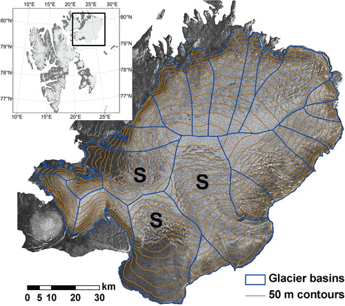
Austfonna (7800 km²) is located on the Nordaustlandet island in the north-east of the Svalbard Archipelago (Fig. 1). The ice cap geometry is characterized by one major ice dome which rises gently up to about 800 m a.s.l. and feeds a number of drainage basins. Apart from a few fast-flowing units, most of the ice cap is slow-moving with typical velocities less than 10 m y⁻¹ (Dowdeswell et al. 1999; Strozzi et al. 2008). Glacier surges have been reported for three of the basins (Fig. 1), but not during the last 70 years (Lefauconnier & Hagen 1991). The most detailed mapping of Austfonna was done in 1983 by airborne radio echo-sounding (RES) (Dowdeswell et al. 1986). Surface and bedrock elevations were obtained along a dense grid of altimetry profiles. It was found that 30% of the ice cap is grounded below sea level, with ice thicknesses ranging from <300 m in the marine south-east to 500 m in the interior. The RES surface elevations were used by the Norwegian Polar Institute to improve their topographic map series (NPI 2011). Others have made DEMs of Austfonna based on DInSAR (Unwin & Wingham 1997) and optical shape-from-shading applied to Landsat imagery (Bingham & Rees 1999). Owing to the lack of more recent GCPs, both of these DEMs were tied to a selection of 1983 RES data with relative accuracies of 8 and 14 m, respectively. Recent elevation data from ICESat, airborne laser altimetry and GNSS surface profiles indicate that the RES-dependent DEMs are systematically 30–50 m too low in the summit area and 10–30 m too high close to the margins. These deviations can be partly explained by interior thickening and peripheral thinning (Bamber et al. 2004), but there might also be an elevation-dependent bias in the 1983 data related to the pressure-altitude recordings (Moholdt 2010). The large deviation between existing DEMs and the current geometry implies a need for a new baseline DEM to be used in current and future glaciological work at Austfonna.

Fig. 1  Glacier topography (50 m contour interval) and drainage basins of Austfonna derived from the DInSAR/ICESat digital elevation model. An orthorectified version of a synthetic aperture radar intensity image from 5 March 1996 is also shown. The inset map shows the location of Austfonna (79.8°N, 24°E) in Svalbard. Glacier basins that are known to have surged are indicated with an S.

Data sets

Most SAR satellites have a repeat pass period of 10–50 days (Rott 2009), which limits the phase coherence over temporally variable surfaces like glaciers. Shorter repeat-times are available for the three-day ice phase of the first European Remote Sensing Satellite (ERS-1) in winter 1992 and 1994, and from the tandem phase of ERS-1/2 in 1995–96 when ERS-2 was following the ERS-1 orbit at a 24-h delay. We selected two tandem SAR image pairs from a descending track covering the entire Austfonna with baseline configurations that are beneficial for extracting topographic phases from DInSAR (Table 1, Fig. 2). The same set of SAR scenes have previously been used to estimate down-slope surface velocities across the ice cap (Bevan et al. 2007). Other InSAR studies at Austfonna (Unwin & Wingham 1997; Dowdeswell et al. 1999; Dowdeswell et al. 2008; Strozzi et al. 2008) have used SAR scenes from satellite tracks where the image frames do not cover the entire ice cap. Our selection of scenes avoids the problem of mosaicing between incoherent interferograms from different satellite tracks. The SAR data were delivered by the European Space Agency (ESA) as pre-processed single-look complex (SLC) images that contain both amplitude and phase information. Partly overlapping SLC frames from the same satellite pass were merged together ahead of the interferometric processing to obtain scenes with full ice cap coverage. This was done by resampling the second frame into the geometry of the first frame based on the azimuth offset, which was estimated by image cross-correlation between the corresponding intensity images. Finally, we replaced the original ESA satellite ephemerides with precise post-processed ERS-1/2 orbits obtained from the Delft University of Technology (Scharroo & Visser 1998).

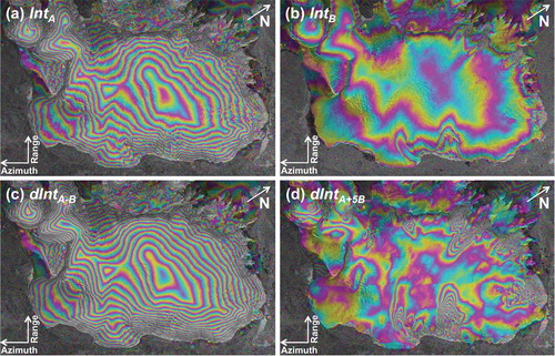
Fig. 2  Two-pass interferograms (Int) and smoothed combined interferograms (dInt): (a) Int _A from 5–6 March 1996 with dominating topographic fringes (B _⊥ ca. 178 m), (b) Int _B from 9–10 April 1996 with some visible movement fringes (B _⊥ ca. 34 m), (c) dInt _A-B with topography only (B _⊥ ca. 212 m), and (d) dInt _A + 5B with most topography removed (B _⊥ ca. 8 m) and upscaled movement fringes remaining.

The Geoscience Laser Altimeter System (GLAS) onboard ICESat acquires surface elevations from ground footprints of ca. 70 m diameter spaced at ca. 170 m along each track (Zwally et al. 2002). Elevation accuracies of a few centimetres have been demonstrated under optimal conditions (Fricker et al. 2005), but the performance degrades over sloping terrain and under conditions favourable to atmospheric forward scattering and detector saturation (Brenner et al. 2007). An elevation precision of less than 0.5 m has been found from crossover points within individual ICESat observation campaigns (<35 days) at Austfonna (Moholdt, Hagen et al. 2010). We used the GLA06 altimetry product release 31 which is based on the ice sheet waveform parametrization (Zwally et al. 2010). Ground control points were selected from a subset of ICESat observations collected in the February/March observation campaign in 2006, 2007 and 2008. Priority was given to the observations with the lowest detector gain setting whenever data were available from multiple profiles along the same ICESat reference track. Gain thresholds are commonly used as cloud filters to remove observations susceptible to forward scattering (Yi et al. 2005; Brenner et al. 2007).

The boundary of the glacier DEM was determined from optical satellite imagery. New glacier outlines were manually digitized from an orthorectified SPOT-5 2008 scene (Korona et al. 2009) covering the northern and western margins of the ice cap and a Landsat-7 2001 scene covering the tidewater front to the south-east (Fig. 3). The total ice cap area was calculated to be 7800 km², which is less than previously published values (Hagen et al. 1993) but consistent with the general glacier front retreat of a few tens of metres per year over the past few decades (Dowdeswell et al. 2008).

Fig. 3  Validation of the digital elevation model (DEM) with respect to ICESat ground control points from winter 2006–08 (profiles with no outlines), Global Navigation Satellite Systems surface profiles and airborne light detection and ranging (LIDAR) (black outlines). The vertical root mean square error of the DEM was 9–11 m with respect to each of the three reference data sets (Fig. 4). The underlying images are a SPOT-5 scene from 14 August 2008 and a Landsat-7 scene from 10 July 2001 which were used to digitize new glacier outlines.

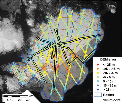
Independent surface elevation profiles from surface GNSS and airborne laser altimetry acquired in spring 2007 were used to validate the DEM (Fig. 3). The GNSS data were obtained from a dual-frequency receiver mounted on a tripod on a sledge which was pulled by a snowmobile (Eiken et al. 1997). The measurements were differentially post-corrected against a base station at the summit. Airborne light detection and ranging (LIDAR) data were collected in diagonal swipes within a 300 m wide ground swathe (Forsberg et al. 2002). Most of the LIDAR profiles were overlapping with the GNSS profiles, yielding a relative elevation accuracy of a few decimetres which is more than sufficient for DEM validation purposes. The GNSS and LIDAR data were separately averaged within 50 m clusters to obtain a comparable resolution to the DInSAR/ICESat DEM.

DInSAR processing

The procedure for deriving glacier topography from differential SAR interferometry is well established (Joughin et al. 1996; Kwok & Fahnestock 1996). The four-pass DInSAR processing was done in the Gamma Remote Sensing software (Wegmüller & Werner 1997) in a stepwise manner: (1) co-registration of SLC image pairs (Img _A1 vs. Img _A2 and Img _B1 vs. Img _B2 , Table 1); (2) generation of multi-look (2×range, 10×azimuth) complex interferograms (Int _A and Int _B ); (3) calculation of baselines (B) and removal of phase trends from the curved Earth (flattening, Fig. 2a,b); (4) co-registration of the interferograms (Int _A vs. Int _B ) using their intensity images; (5) topographic phase isolation by interferogram differencing (dInt _A-B =Int _A –Int _B ) (Fig. 2c); and (6) adaptive filtering and phase unwrapping using the branch-cut algorithm (dInt _A-B => dInt _unw ). Image offsets for the co-registration of SLC images and interferograms were estimated to an accuracy of better than 0.1 pixels by cross-correlating the corresponding intensity images at a decreasing number of multi-looks. The flattened interferograms contain phase differences that are due to topography, movement and noise (Fig. 2a,b). The topographic phase contribution in an interferogram increases with an increasing perpendicular baseline (B _⊥ ) while the phase contribution from surface movement is independent from the baseline. Hence, it is possible to remove the effect from glacier movement by differential InSAR assuming that the line-of-sight velocities are similar in both interferograms (Fig. 2c). Continuous GNSS measurements of stake positions in two dynamic basins on Austfonna show that surface velocities were fairly stable during winter 2009 and 2010 (Dunse 2011).

Table 1 The three interferograms that were generated and their associated pairs of ERS-1/2 tandem synthetic aperture radar scenes with satellite track number, acquisition dates and baseline lengths of the parallel (B _|| ) and perpendicular (B _⊥ ) components at the interferogram centre point. The third interferogram (dInt _A-B ) is a differential interferogram between the two first ones (Int _A –Int _B ).

Interferogram	Track	Date 1	Date 2	B ||	B ⊥
Int A	223 desc.	5 Mar 1996	6 Mar 1996	78 m	178 m
Int B	223 desc.	9 Apr 1996	10 Apr 1996	−13 m	−34 m
Dint A-B	223 desc.	5–6 Mar 1996	9–10 Apr 1996	91 m	212 m

The most critical step in DInSAR processing is phase unwrapping. It is the process of adding the correct multiple of 2π to the interferogram fringes which are otherwise only known modulo 2π. We used a branch-cut algorithm (Goldstein et al. 1988) which isolates potential discontinuities in the interferogram and then unwraps along paths of integration between the branch-cut barriers. The phase coherence was mostly good for both interferograms, and the gentle slope and smooth surface of the ice cap surface ensures a good continuity between the fringes. The resulting unwrapped interferogram (dInt _unw ) defines a topographic surface of absolute phases at a combined perpendicular baseline of 212 m (Table 1), corresponding to a topographic sensitivity of about 50 m per fringe.

DEM generation

The unwrapped phases of the topographic interferogram (dInt _unw ) were transformed into real elevations and a geocoded DEM through the following steps: (1) transformation of ICESat GCPs from UTM coordinates to SAR coordinates (range, azimuth); (2) least-squares baseline refinement using the transformed ICESat GCPs; (3) phase-to-height transformation and geocoding into map geometry (UTM); (4) removal and smoothing of topographic inconsistencies (erroneous holes and cliffs); and (5) resampling into a 50×50 m DEM and clipping to the glacier outlines (Fig. 1).

Precise Delft ephemerides were used to transform the ICESat GCPs from map to SAR geometry and to geocode the DEM from SAR to map geometry. We also attempted to refine the geocoding by matching one of the SAR intensity images with a simulated intensity image from an external DEM in map geometry, but that proved difficult due to the large fraction of uncorrelated surfaces over the ice cap and the ocean. The quality of the geocoding was instead evaluated by checking for correlations between aspect and elevation deviation (normalized by slope) between the geocoded DEM and ICESat (Nuth & Kääb 2011). No significant trends were found, and the corresponding orthorectified intensity image (Fig. 1) fitted well to the coastline and glacier outlines. We did not therefore perform any further geo-referencing of the DEM. Higher-order geo-referencing is precarious at Austfonna due to the lack of ground reference on the south-east side of the ice cap.

Although the Delft orbits have an estimated radial root mean square (RMS) error of only 5 cm (Scharroo & Visser 1998), the baseline uncertainty will still have a major impact on the precision of the topographic surface of unwrapped phases. The height-equivalent RMS error of the linear fit between ICESat GCPs and unwrapped phases decreased from ca. 40 m to ca. 10 m after the refinement of the interferometric baseline. The refinement procedure optimizes the baseline coordinates (along-track, cross-track and normal) at each point along the SAR track based on a non-linear least-squares solution of the fit between unwrapped phases and elevations at GCP locations. Hence, the baseline parameters are not necessarily adjusted to the exact SAR acquisition geometry of 1996, but rather to the optimal baseline configuration for fitting the DEM with the GCPs from 2006 to 2008. Ideally, we should have used GCPs and SAR scenes acquired at the same time. A few airborne laser profiles are available from spring 1996 (Bamber et al. 2004), but unfortunately the spatial coverage was not sufficient to refine precise baseline parameters across the whole ice cap.

Discontinuous phases and errors in the phase unwrapping can cause data gaps and elevation jumps in the resulting DEM. The entire ice cap interior was continuous and smooth, but a few smaller data voids and topographic inconsistencies were present along the margins. We suspected that pixels with a DEM-derived surface slope higher than 10° were erroneous. These pixels were classified as data voids and then filled in linearly from the surrounding pixels. Surface slopes were then calculated over again, and new error areas were identified. This process was repeated iteratively until all slopes were brought below 10°. About 1% of the pixels were interpolated in this way, and the maximum interpolation distance was 500 m.

The main DEM was produced from GCPs with orthometric heights (above sea level) relative to the EGM2008 geoid. Since most satellite systems operate in ellipsoidic reference systems, we also constructed a DEM with ellipsoidic heights relative to the WGS84 ellipsoid. The ICESat GCP coordinates were first transformed from the TOPEX/Poseidon ellipsoid to the WGS84 ellipsoid, and then the DEM was generated in the same way as for the orthometric DEM. The DEM validation with respect to GNSS and LIDAR data was done for the ellipsoidic DEM rather than transforming the data into orthometric heights. The geoid height of EGM2008 with respect to the WGS84 ellipsoid varies from 25 to 29 m across Austfonna from the east to the west.

DEM validation and errors

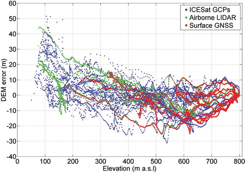
The DEM was validated against ICESat GCPs and independent surface profiles from GNSS and airborne LIDAR (Figs. 3, 4). The point elevations were compared with the DEM by means of bilinear interpolation, yielding 5–6000 points of comparison for each data set. The mean bias of the DEM was close to zero for the ICESat and LIDAR data sets and –4 m for the GNSS data set. The standard deviations were 11 m, 10 m and 8 m respectively. The larger bias and smaller standard deviation of the GNSS comparison is because the GNSS profiles are spatially biased towards the higher elevations of the ice cap (Fig. 4). The ICESat data set has the best spatial coverage for validation, but there is a dependency between the ICESat GCPs and the DEM since they are used to refine the baseline parameters. The preferred error estimator is therefore airborne LIDAR, which indicates a DEM precision of roughly 10 m with no significant overall bias.

Fig. 4  Elevation differences between the digital elevation model (DEM) and the three validation data sets: ICESat ground control points (GCPs), airborne light detection and ranging (LIDAR) and surface Global Navigation Satellite Systems (GNSS) profiles. The root mean square error of the DEM with respect to the three data sets is 11 m, 10 m and 9 m, respectively. The spatial distribution of the data can be seen in Fig. 3.

DEM errors can be due to low phase coherence, atmospheric disturbance, residual glacier movement, signal penetration and temporal elevation change. The baseline refinement procedure adjusts the DEM to the average elevation of the GCPs and accounts for elevation errors that vary linearly with elevation. Such elevation-dependent errors can be atmospheric disturbances and spatial variations in signal penetration and temporal elevation change. Elevation changes between the 1996 SAR acquisitions and the 2006–08 ICESat observations are probably on the order of ±5–10 m with thickening in the interior and thinning towards the margins (Bamber et al. 2004; Moholdt, Hagen et al. 2010). Most of this regular pattern should be incorporated in the baseline refinement, but local and non-linear elevation changes will remain in the resulting DEM. The elevation bias from the penetration of SAR signals into snow and ice will be corrected for the average penetration-depth and potential linear trends with elevation. The depth of the C-band phase centre is less than a few metres in exposed ice, but it can be up to 10 m in cold and dry firn (Rignot et al. 2001). Surface profiles with C-band ground-penetrating radar at Svalbard have shown a variation in the phase-centre depth from about 1 m in the ablation area to up to 5 m in the firn area (Müller 2011). The effect of small-scale errors like speckle noise has most likely been reduced by the multi-look averaging in the interferogram generation and the adaptive filtering prior to the phase unwrapping.

The DEM is consistently too high in the lowermost parts of the ice cap (Figs. 3, 4). This is probably due to a strong frontal thinning of 1–3 m y⁻¹ which is not compensated by the baseline refinement because the relation between elevation and elevation change has more of a curved trend than a linear trend at Austfonna (Moholdt, Hagen et al. 2010). The elevation overestimation along the margins is compensated by a slight underestimation in the interior, especially in the three known surge-type basins in the central south (Figs. 1, 3). These quiescent basins might have been thickening faster than the other basins (Bamber et al. 2004; Bevan et al. 2007) although this was not evident between 2002 and 2008 (Moholdt, Hagen et al. 2010).

DEMs can be used to derive maps of slope, aspect and topographic shading (e.g., Wilson & Gallant 2000) which can further be used to validate the DEM. The slope precision of the DEM is estimated to about 0.3° at spatial scales of 50–200 m as compared with slopes derived from GNSS and ICESat. Compared to ICESat repeat-track planes (Moholdt, Nuth et al. 2010), the standard deviation of slopes and aspects are 0.5° and 24°, respectively. The mean slope difference was close to zero in both cases, indicating a similar degree of smoothness between the data sets. The variation in slope and aspect across Austfonna is visualized in a hillshade model in Fig. 5. The major drainage divides can be clearly identified, as well as some areas with rolling topography and phase noise.

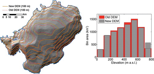
Fig. 5  A comparison of contour lines for the new and old digital elevation models (DEM) of Austfonna. The old DEM is a smoothed merge (K. Melvold, pers. comm.) of the radio-echo-sounding-tied InSAR DEM (Unwin & Wingham 1997) and photogrammetric data from the Norwegian Polar Institute (2011). The corresponding glacier hypsometries for 100 m elevation bins are shown to the right. The contour lines are underlain by a hillshade model of the new DEM, showing the major drainage divides of the ice cap.

The quality of the DEM could potentially have been improved by additional smoothing and bias corrections. We tried applying a low-pass mean filter to reduce small-scale noise, but it did not improve the overall precision of the DEM nor the local slope correspondence between the DEM and pairs of neighbouring ICESat observations separated by ca. 170 m. Hence, we concluded that the DEM was already sufficiently smooth. The elevation-dependent bias in the DEM could have been removed by fitting a curve to the errors in Fig. 4 and correcting the DEM elevations accordingly. This would have improved the precision of the DEM by about 2 m, but we chose to keep it in the original format rather than applying empirical adjustments that might not apply everywhere.

The two previous Austfonna DEMs from DInSAR (Unwin & Wingham 1997) and from optical shape-from-shading (Bingham & Rees 1999) have been reported to have elevation precisions of 8 m and 14 m with respect to the 1983 RES data. The precision of the DInSAR DEM was, however, calculated over a small rectangular area in the interior of the ice cap where the quality of the RES data was best. The standard deviation of the DEM increased to 42 m if all RES data were included in the comparison, but part of this uncertainty is due to the rough RES elevations which have a precision of 17 m as calculated from 256 crossover points. Recent optical stereo DEMs from the International Polar Year (IPY) project SPOT 5 Stereoscopic Survey of Polar Ice: Reference Images and Topographies (SPIRIT; Korona et al. 2009) and the Advanced Spaceborne Thermal Emission and Reflection Radiometer Global DEM (ASTER GDEM) project (Fujisada et al. 2005) have good precision in glacier areas with high image correlation, but the usage of these DEMs at Austfonna is so far limited by holes and artefacts in the summit area where the image matching has failed.

DEM applications

DEMs have a wide range of applications in glaciology. They are used to orthorectify satellite imagery, to remove topographic fringes from displacement interferograms, and to convert slant range and azimuth displacements in SAR interferometry or feature tracking to downslope displacements (e.g., Strozzi et al. 2002). Slopes and aspects derived from DEMs are input parameters for calculating incoming solar radiation at a particular location in surface mass balance models (Hock 1999; Schuler et al. 2007). Surface slopes are also used to calculate driving stresses in studies of glacier dynamics (Dowdeswell 1986; Dunse et al. 2011). Local surface slopes are essential for elevation change analysis of repeat-track satellite altimetry if a DEM is used to correct for the cross-track slope between near repeat-tracks (Slobbe et al. 2008; Moholdt, Hagen et al. 2010). The average slope of the Austfonna DEM was calculated to 1.4°, which infers a relative elevation difference of 2.4 m between two parallel tracks separated by 100 m. Such cross-track elevation differences need to be corrected in order to detect elevation changes of less than a metre. The DEM has already been applied for this purpose in two studies of repeat-track ICESat elevation changes (Moholdt, Hagen et al. 2010; Moholdt, Nuth et al. 2010).

Glacier drainage basins can be determined from a DEM by assuming down-slope movement of ice. Accurate basin outlines are important for studies of glacier dynamics (Dowdeswell 1986; Bevan et al. 2007) and surface mass balance (Moholdt, Hagen et al. 2010). DEM-derived maps of aspect, slope and topographic shading were used to update the existing basin outlines (Dowdeswell 1986; Hagen et al. 1993) to the current geometry (Fig. 1). The basins were further adjusted according to visual ridges in the SPOT-5 and Landsat-7 scenes (Fig. 3) and the SAR intensity images (Fig. 1). The digitized basin outlines were finally checked against the scaled movement interferogram dInt _A + 5B (Fig. 2d) to ensure that the topographic divides were consistent with the dynamic divides. The detectable glacier flow fields generally fitted well to the topographic basins, so no further adjustments were necessary.

Glacier hypsometry is the distribution of glacier area with elevation. Hypsometry is a major control on the glacier-wide surface mass balance, and it is often used to extrapolate elevation-dependent measurements to unsampled glacier areas. We calculated glacier areas within 100 m elevation bins for the new and old Austfonna DEM (Fig. 5). Although the lower elevations have been thinning over the past few decades (Bamber et al. 2004; Moholdt, Hagen et al. 2010), there is no apparent change in the hypsometry at the lowermost elevations due to the simultaneous retreat of the tidewater fronts (Dowdeswell et al. 2008). At medium elevations (200–600 m), the new DEM has slightly smaller areas than the old one, which is fully compensated by a 65% higher area in the uppermost bin (700–800 m). The maximum elevation of the new DEM is 800 m (a.s.l.) whereas it is only 760 m for the old DEM. The impact of the hypsometric difference on surface mass balance extrapolations is large locally in the summit area, but only 0.01 m w.e. y⁻¹ on average when a specific balance of 0.5 m w.e. y⁻¹ (Pinglot et al. 2001) in the uppermost bin is averaged over the entire ice cap area. Assuming a constant climate, the long-term hypsometric trend of interior thickening combined with peripheral thinning and retreat will cause an increasingly positive specific surface mass balance until it is compensated by glacier acceleration or surging.

Conclusions

We have generated a new DEM of Austfonna by performing differential SAR interferometry (DInSAR) on two pairs of ERS-1/2 tandem images from 1996. The precision of DInSAR DEMs depends mainly on the length and accuracy of the interferometric baseline. We used ICESat laser altimetry from winter 2006–08 as GCPs to refine the baseline parameters. ICESat is ideal for this purpose since it provides accurate surface elevations at a homogeneous spatial distribution. The baseline refinement with ICESat improved the precision of the DEM from ca. 40 m to ca. 10 m as compared to ICESat GCPs and independent surface profiles from GNSS and airborne LIDAR. The DEM has no significant overall bias, but there is an elevation-dependent bias with too high elevations along the margins and slightly too low elevations in the interior. This is most likely due to non-linear elevation change in the decade between the SAR and ICESat acquisitions. With the availability of coincident SAR and altimetry data from new satellite systems like TanDEM-X (Krieger et al. 2007) and CryoSat-2 (Wingham et al. 2006), it will probably be possible to generate ice cap DEMs in a similar way with significantly better accuracies than in this study.

The new Austfonna DEM has proven useful for elevation change studies where multitemporal ICESat altimetry data need to be corrected for the cross-track slope between near repeat-tracks (Moholdt, Hagen et al. 2010; Moholdt, Nuth et al. 2010). It is also well suited for delineating glacier drainage basins and calculating glacier hypsometries. The new glacier DEM and basin outlines will serve as a baseline data set for future and ongoing research on Austfonna, including surface mass balance monitoring and modelling, studies of glacier dynamics and elevation change analysis. All data presented here will be freely available through the University of Oslo and the IPY project Dynamic Response of Arctic Glaciers to Global Warming (GLACIODYN).

Acknowledgements

This work was supported by funding to the CryoSat Calibration and Validation Experiment (CryoVEX), the IPY GLACIODYN project and the Ice2sea programme within the European Union Seventh Framework Programme (grant no. 226375, Ice2sea contribution no. 018). GM was also supported through an Arctic Field Grant from the Svalbard Science Forum. We are thankful to the numerous data contributors, namely the European Space Agency proposal AOCRY.2683 (SAR data), the Delft University of Technology (ERS ephemerides), the National Snow and Ice Data Center (ICESat data), the National Space Institute at the Technical University of Denmark (LIDAR data), the US Geological Survey GloVis (Landsat data), the IPY SPIRIT project, the US National Aeronautical and Space Administration and Japan's Ministry of Economy, Trade and Industry (ASTER GDEM), the Norwegian Polar Institute (topographic data), and to J. Dowdeswell and T. Benham (RES data). Fieldwork at Austfonna is a joint project between the University of Oslo and the Norwegian Polar Institute, and all participants are acknowledged. We also thank C. Nuth for helping out with the DEM validation.

References

- Arnold N.S. Rees W.G. Devereux B.J. Amable G.S. Evaluating the potential of high-resolution airborne LiDAR data in glaciology. International Journal of Remote Sensing. 2006; 27: 1233–1251. 10.3402/polar.v31i0.18460.
- Baek S. Kwoun O.I. Braun A. Lu Z. Shum C.K. Digital elevation model of King Edward VII Peninsula, West Antarctica, from SAR interferometry and ICESat laser altimetry. IEEE Geoscience and Remote Sensing Letters. 2005; 2: 413–417. 10.3402/polar.v31i0.18460.
- Bamber J, Krabill W, Raper V. & Dowdeswell J. 2004. Anomalous recent growth of part of a large Arctic ice cap: Austfonna, Svalbard. Geophysical Research Letters 31. , L12402, 10.3402/polar.v31i0.18460.
- Bevan S. Luckman A. Murray T. Sykes H. Kohler J. Positive mass balance during the late 20th century on Austfonna, Svalbard, revealed using satellite radar interferometry. Annals of Glaciology. 2007; 46: 117–122. 10.3402/polar.v31i0.18460.
- Bingham A.W. Rees W.G. Construction of a high-resolution DEM of an Arctic ice cap using shape-from-shading. International Journal of Remote Sensing. 1999; 20: 3231–3242. 10.3402/polar.v31i0.18460.
- Brenner A. C. DiMarzio J.R. Zwally H.J. Precision and accuracy of satellite radar and laser altimeter data over the continental ice sheets. IEEE Transactions on Geoscience and Remote Sensing. 2007; 45: 321–331. 10.3402/polar.v31i0.18460.
- Dall J. Madsen S.N. Keller K. Forsberg R. Topography and penetration of the Greenland ice sheet measured with airborne SAR interferometry. Geophysical Research Letters. 2001; 28: 1703–1706. 10.3402/polar.v31i0.18460.
- DiMarzio J. Brenner A. Schutz B. Shuman C.A. Zwally H.J. GLAS/ICESat laser altimetry digital elevation models of Greenland (1 km) and Antarctica (500 m). Digital media. National Snow and Ice Data Center. Boulder, 2007
- Dowdeswell J.A. Drainage-basin characteristics of Nordaustlandet ice caps, Svalbard. Journal of Glaciology. 1986; 32: 31–38.
- Dowdeswell J.A, Benham T.J, Strozzi T. & Hagen J.O. 2008. Iceberg calving flux and mass balance of the Austfonna ice cap on Nordaustlandet, Svalbard. Journal of Geophysical Research—Earth Surface 113. F03022., 10.3402/polar.v31i0.18460.
- Dowdeswell J.A. Drewry D.J. Cooper A.P.R. Gorman M.R. Liestøl O. Orheim O. Digital mapping of the Nordaustlandet ice caps from airborne geophysical investigations. Annals of Glaciology. 1986; 8: 51–58.
- Dowdeswell J.A. Unwin B. Nuttall A.M. Wingham D.J. Velocity structure, flow instability and mass flux on a large Arctic ice cap from satellite radar interferometry. Earth and Planetary Science Letters. 1999; 167: 131–140. 10.3402/polar.v31i0.18460.
- Drews R. Rack W. Wesche C. Helm V. A spatially adjusted elevation model in Dronning Maud Land, Antarctica, based on differential SAR interferometry. IEEE Transactions on Geoscience and Remote Sensing. 2009; 47: 2501–2509. 10.3402/polar.v31i0.18460.
- Dunse T. 2011. Glacier dynamics and subsurface classification of Austfonna, Svalbard: interferences from observations and modelling. PhD thesis, University of Oslo.
- Dunse T. Greve R. Schuler T.V. Hagen J.O. Permanent fast flow versus cyclic surge behavior: numerical simulations of the Austfonna ice cap, Svalbard. Journal of Glaciology. 2011; 57: 247–259. 10.3402/polar.v31i0.18460.
- Eiken T. Hagen J.O. Melvold K. Kinematic GPS survey of geometry changes on Svalbard glaciers. Annals of Glaciology. 1997; 24: 157–163.
- Forsberg R, Keller K. & Jacobsen S.M. 2002. Airborne lidar measurements for Cryosat validation. In: IEEE International Geoscience and Remote Sensing Symposium: 24th Canadian symposium on remote sensing. Vol. 3. Pp. 1756–1758. New York: Institute of Electrical and Electronics Engineers.
- Fricker H.A, Borsa A, Minster B, Carabajal C, Quinn K. & Bills B. 2005. Assessment of ICESat performance at the Salar de Uyuni, Bolivia. Geophysical Research Letters. 32, L21S06, 10.3402/polar.v31i0.18460.
- Fujisada H. Bailey G.B. Kelly G.G. Hara S. Abrams M.J. ASTER DEM performance. IEEE Transactions on Geoscience and Remote Sensing. 2005; 43: 2707–2714. 10.3402/polar.v31i0.18460.
- Goldstein R.M. Zebker H.A. Werner C.L. Satellite radar interferometry—two-dimensional phase unwrapping. Radio Science. 1988; 23: 713–720. 10.3402/polar.v31i0.18460.
- Hagen J.O. Liestol O. Roland E. Jorgensen T. Glacier atlas of Svalbard and Jan Mayen. Meddelelser 129. Norwegian Polar Institute. Oslo, 1993
- Hock R. A distributed temperature-index ice- and snowmelt model including potential direct solar radiation. Journal of Glaciology. 1999; 45: 101–111.
- Joughin I. Winebrenner D. Fahnestock M. Kwok R. Krabill W. Measurement of ice-sheet topography using satellite radar interferometry. Journal of Glaciology. 1996; 42: 10–22.
- Kääb A. Glacier volume changes using ASTER satellite stereo and ICESat GLAS laser altimetry. A test study on Edgeoya, eastern Svalbard. IEEE Transactions on Geoscience and Remote Sensing. 2008; 46: 2823–2830. 10.3402/polar.v31i0.18460.
- Korona J. Berthier E. Bernard M. Remy F. Thouvenot E. SPIRIT. SPOT 5 Stereoscopic Survey of Polar Ice: Reference Images and Topographies during the fourth International Polar Year (2007–2009). ISPRS Journal of Photogrammetry and Remote Sensing. 2009; 64: 204–212. 10.3402/polar.v31i0.18460.
- Krieger G. Moreira A. Fiedler H. Hajnsek I. Werner M. Younis M. Zink M. TanDEM-X: a satellite formation for high-resolution SAR interferometry. IEEE Transactions on Geoscience and Remote Sensing. 2007; 45: 3317–3341. 10.3402/polar.v31i0.18460.
- Kwok R. Fahnestock M.A. Ice sheet motion and topography from radar interferometry. IEEE Transactions on Geoscience and Remote Sensing. 1996; 34: 189–200. 10.3402/polar.v31i0.18460.
- Lefauconnier B. Hagen J. O. Surging and calving glaciers in eastern Svalbard. Meddelelser 116. Norwegian Polar Institute. Oslo, 1991
- Moholdt G. 2010. Elevation change and mass balance of Svalbard glaciers from geodetic data. PhD thesis, University of Oslo.
- Moholdt G. Hagen J.O. Eiken T. Schuler T. V. Geometric changes and mass balance of the Austfonna ice cap, Svalbard. The Cryosphere. 2010; 4: 21–34. 10.3402/polar.v31i0.18460.
- Moholdt G. Nuth C. Hagen J.O. Kohler J. Recent elevation changes of Svalbard glaciers derived from ICESat laser altimetry. Remote Sensing of Environment. 2010; 114: 2756–2767. 10.3402/polar.v31i0.18460.
- Müller K. 2011. Microwave penetration in polar snow and ice: Implications for GPR and SAR. PhD thesis, University of Oslo.
- Norwegian Polar Institute. 2011. Svalbard 1:100 000 (S100). Tromsø: Norwegian Polar Institute.
- Nuth C. Kääb A. Co-registration and bias corrections of satellite elevation data sets for quantifying glacier thickness change. The Cryosphere. 2011; 5: 271–290. 10.3402/polar.v31i0.18460.
- Nuth C. Kohler J. Aas H.F. Brandt O. Hagen J. O. Glacier geometry and elevation changes on Svalbard (1936–90): a baseline dataset. Annals of Glaciology. 2007; 46: 106–116. 10.3402/polar.v31i0.18460.
- Palmer S. J, Sheperd A, Sundal A, Rinne E. & Nienow P. 2010. InSAR observations of ice elevation and velocity fluctuations at the Flade Isblink ice cap, eastern North Greenland. Journal of Geophysical Research. 115, F04037., doi: 10.1029/2010JF001686.
- Pinglot J.F. Hagen J. O. Melvold K. Eiken T. Vincent C. A mean net accumulation pattern derived from radioactive layers and radar soundings on Austfonna, Nordaustlandet, Svalbard. Journal of Glaciology. 2001; 47: 555–566. 10.3402/polar.v31i0.18460.
- Rignot E. Echelmeyer K. Krabill W. Penetration depth of interferometric synthetic-aperture radar signals in snow and ice. Geophysical Research Letters. 2001; 28: 3501–3504. 10.3402/polar.v31i0.18460.
- Rott H. Advances in interferometric synthetic aperture radar (InSAR) in earth system science. Progress in Physical Geography. 2009; 33: 769–791. 10.3402/polar.v31i0.18460.
- Scharroo R. Visser P. Precise orbit determination and gravity field improvement for the ERS satellites. Journal of Geophysical Research—Oceans. 1998; 103: 8113–8127. 10.3402/polar.v31i0.18460.
- Schuler T.V. Loe E. Taurisano A. Eiken T. Hagen J.O. Kohler J. Calibrating a surface mass-balance model for Austfonna ice cap, Svalbard. Annals of Glaciology. 2007; 46: 241–248. 10.3402/polar.v31i0.18460.
- Slobbe D.C. Lindenbergh R.C. Ditmar P. Estimation of volume change rates of Greenland's ice sheet from ICESat data using overlapping footprints. Remote Sensing of Environment. 2008; 112: 4204–4213. 10.3402/polar.v31i0.18460.
- Strozzi T. Kouraev A. Wiesmann A. Wegmüller U. Sharov A. Werner C. Estimation of Arctic glacier motion with satellite L-band SAR data. Remote Sensing of Environment. 2008; 112: 636–645. 10.3402/polar.v31i0.18460.
- Strozzi T. Luckman A. Murray T. Wegmüller U. Werner C.L. Glacier motion estimation using SAR offset-tracking procedures. IEEE Transactions on Geoscience and Remote Sensing. 2002; 40: 2384–2391. 10.3402/polar.v31i0.18460.
- Unwin B. Wingham D. Topography and dynamics of Austfonna, Nordaustlandet, Svalbard, from SAR interferometry. Annals of Glaciology. 1997; 24: 403–408.
- Wegmüller U. Werner C. Gamma SAR processor and interferometry software. Third ERS Symposium on Space at the Service of Our Environment: soil moisture, hydrology, land use, forestry, DEM, geology, hazards. Florence, Italy, 14–21 March 1997. Guyenne T.-D. Danesy D. European Space Agency. Pp. Paris, 1997; 1687–1692.
- Wilson J. Gallant J. Terrain analysis: principles and applications. John Wiley & Sons. New York, 2000
- Wingham D.J. Francis C.R. Baker S. Bouzinac C. Brockley D. Cullen R. de Chateau-Thierry P. Laxon S.W. Mallow U. Mavrocordatos C. Phalippou L. Ratier G. Rey L. Rostan F. Viau P. Wallis D.W. CryoSat: a mission to determine the fluctuations in Earth's land and marine ice fields. Natural Hazards and Oceanographic Processes from Satellite Data. 2006; 37: 841–871.
- Yi D. H. Zwally H.J. Sun X.L. ICESat measurement of Greenland ice sheet surface slope and roughness. Annals of Glaciology. 2005; 42: 83–89. 10.3402/polar.v31i0.18460.
- Zwally H.J. Schutz B. Abdalati W. Abshire J. Bentley C. Brenner A. Bufton J. Dezio J. Hancock D. Harding D. Herring T. Minster B. Quinn K. Palm S. Spinhirne J. Thomas R. ICESats laser measurements of polar ice, atmosphere, ocean, and land. Journal of Geodynamics. 2002; 34: 405–445. 10.3402/polar.v31i0.18460.
- Zwally H.J, Schutz R, Bentley C, Bufton J, Herring T, Minster B, Spinhirne J. & Thomas R. 2010. GLAS/ICESat L1B global elevation data. V031, 20 February 2003 to 11 October 2009. Digital media. Boulder: National Snow and Ice Data Center.