The potential response of the hydrate reservoir in the South Shetland Margin, Antarctic Peninsula, to ocean warming over the 21st century

Abstract

In the South Shetland Margin (SSM), Antarctic Peninsula, a bottom-simulating reflector indicates the presence of hydrate between ca. 500 and 3000 m water depth (mwd). The cold seabed temperatures allow hydrate stability at shallower water depths. During the past five decades, the Antarctic Peninsula has been warming up faster than any other part of the Southern Hemisphere, and long-term ocean warming could affect the stability of the SSM hydrate reservoir at shallow waters. Here, we model the transient response of the SSM hydrate reservoir between 375 and 450 mwd to ocean warming for the period 1958–2100. For the period 1958–2010, seabed temperatures are given by oceanographic measurements in the area, and for 2010–2100 by two temperature scenarios represented by the observed trends for the periods 1960–2010 (0.0034°C y⁻¹) and 1980–2010 (0.023°C y⁻¹). Our results show no hydrate-sourced methane emissions for an ocean warming rate at the seabed of 0.0034 °C y⁻¹. For a rate of 0.023°C y⁻¹, emissions start in 2028 at 375 mwd and extend to 442 mwd at an average rate of about 0.91 mwd y⁻¹, releasing ca. 1.13×10³ mol y⁻¹ of methane per metre along the margin by 2100. These emissions originate from dissociation at the top of the hydrate layer, a physical process that steady-state modelling cannot represent. Our results are speculative on account of the lack of direct evidence of a shallow water hydrate reservoir, but they illustrate that the SSM is a key area to observe the effects of ocean warming-induced hydrate dissociation in the coming decades.

• Hydrate
• ocean warming
• methane emissions
• transient modelling
• South Shetland Margin
• Antarctic Peninsula.

Hydrate is an ice-like compound in which gas molecules are lodged within the clathrate crystal lattice (Sloan & Koh 2008) and is stable at high pressure–low temperature conditions. Hydrate is most sensitive to global warming at high latitudes (e.g., Hunter et al. 2013), and at present there is evidence—in the form of methane bubble plumes emanating from the seabed—of warming-induced hydrate dissociation at ca. 400 m water depth (mwd) offshore west of Svalbard (e.g., Westbrook et al. 2009; Sahling et al. 2014), a process likely to propagate to deeper waters during the 21st century (e.g., Reagan et al. 2011; Marín-Moreno et al. 2015). The seabed waters of the Antarctic Peninsula may be sufficiently cold to allow the formation of hydrate at shallow water depths (less than ca. 450 m), as occurs in the Arctic (e.g., Buffett & Archer 2004), if the dissolved methane concentration in the pore water, within the hydrate stability zone (HSZ), is at or above saturation value.

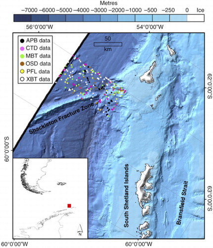
In the past five years, scientists interested in modelling warming-induced hydrate dissociation have almost exclusively focused on the Arctic, perhaps underestimating the importance of this process in other potential sensitive areas of our planet, such as the South Shetland Margin (SSM), Antarctic Peninsula (Fig. 1). In the SSM, multichannel seismic reflection profiles and ocean bottom seismograph data were acquired during the Italian Antarctic expeditions in the Austral summers 1989/90 (Lodolo et al. 1993), 1996/97 (Lodolo et al. 2002), and 2004/05 (Tinivella et al. 2008) in water depths ranging between 500 and 5000 m. During these expeditions, a strong and continuous bottom-simulating reflector (BSR; Shipley et al. 1979) was identified between ca. 500 and 3000 mwd. This BSR has been associated with the presence of a gas reservoir below the hydrate (e.g., Tinivella & Accaino 2000; Tinivella et al. 2009; Loreto & Tinivella 2012) and with diagenetic alteration of biogenic silica—Opal-A/Opal-CT transition (Neagu et al. 2009)—as suggested by Ocean Drilling Program Leg 178 results near the area (e.g., Volpi et al. 2003). North-east of the Antarctic Peninsula, in the central and southern Scotia Sea, three different BSRs caused by Opal-A/Opal-CT transition (deep), Opal-CT/Quartz transition (middle) and gas/hydrate contact (shallow) have been also identified (Somoza et al. 2014). In this area, both the breaching of diagenetic BSRs and the presence of a hydrate-related BSR may indicate the formation of sub-seabed hydrate by upwards migration of gas from a deep reservoir through faults (Somoza et al. 2014). Here we assume a gas/hydrate-related BSR, and that the associated gas and hydrate reservoirs can be extended to shallower water depths where the thermodynamic conditions for hydrate stability are satisfied.

Fig. 1  Bathymetric map (Arndt et al. 2013) with seabed temperature measurements at our study location in the South Shetland Margin (red square in the inset) downloaded from the National Oceanographic Data Center (www.nodc.noaa.gov/cgi-bin/OC5/WOA09/woa09.pl). The seabed temperatures are from: autonomous pinniped bathythermograph (APB) data; high and bottle-low resolution conductivity–temperature–depth (CTD) and expendable CTD (XCTD) data; mechanical/digital bathythermograph (MBT and DBT, respectively) and expendable bathythermograph (XBT) data; ocean station data (OSD); profiling float (PFL) data. The map is projected with the coordinate system Polar Stereographic 65°S (Datum: WGS84).

The sedimentary deposits of the Antarctic Peninsula capture the influence of bottom-current processes along the seafloor and show contouritic drifts and erosional features (e.g., Maldonado et al. 2014). The only proximal borehole to our study area is located east of the SSM, in the Jane Basin, and comprises hemipelagic and pelagic sediments on the top 300 m (site 697B; Barker et al. 1988). Seismic data shows polygonal faults in the central and southern Scotia Sea (Somoza et al. 2014), reverse faults at the foot of the SSM and mass transport deposits especially over the margins of the banks (Maldonado et al. 2014).

Over the period 1958 to 2008, the Antarctic Peninsula shows an unusually high rate of warming (Mulvaney et al. 2012), the strongest of the Southern Hemisphere and one of three strongest on Earth (Vaughan et al. 2003). Predicting future warming in this area is challenging because of the lack of a sound physical mechanism that explains the present regional warming (Vaughan et al. 2003), but some models predict that in the 21st century the Antarctic Peninsula may not experience the strongest warming of Antarctica (Chapman & Walsh 2007). Ocean warming in West Antarctica is predicted to be of 0.5±0.4°C by 2100, about half of global mean warming, considering the A1B scenario (Yin et al. 2011), which assumes modest reductions in greenhouse-gas emissions after mid-21st century. A long-term ocean warming similar to that predicted in West Antarctica may be sufficient to trigger dissociation of a shallow hydrate reservoir in the SSM. This hypothesis has been previously tested by Tinivella et al. (2011) based on steady-state modelling of the evolution of the base of the HSZ assuming a 1°C increase by the end of the 21st century.

Here we model the transient response to ocean warming of the hydrate system in the SSM between 375 and 450 mwd for the period 1958–2100 CE, using constraints in input parameters from seismic observations (Tinivella et al. 2011). Our focus on a single geographical area that has been well characterized geophysically means we make fewer assumptions about the physical parameters involved. The models employ the TOUGH+HYDRATE (T+H) code (Moridis et al. 2012), with past temperatures given by the US National Oceanographic Data Center and two future temperature scenarios given by extrapolation of the temperature trends over the periods 1960–2010 and 1980–2010. For comparison, we also model the steady-state response of the system using Moridis’ (2003) stability curve. To our knowledge, this is the first dynamic modelling study of ocean warming-induced hydrate dissociation in what is today Antarctica's most sensitive area to the effects of global warming (Vaughan et al. 2003; Chapman & Walsh 2007). Our results likely represent an upper-bound scenario of potential future hydrate dissociation offshore Antarctica.

One-dimensional transient modelling approach

Processes modelled

We ran one-dimensional (1D) T+H models for water depths of 375, 400, 425 and 450 m. A model at 350 mwd was also tested, but the hydrate was not stable with the initial pressure and temperature conditions. We adopted a 1D approach because in the SSM between 300 and 500 mwd the slope is about 1°, and differences between 1D and 2D results for such gentle slope and low hydrate saturations (Table 1) are minor (Reagan et al. 2011). Besides, Thatcher et al. (2013) states that an aquifer with a 1° slope generates a horizontal component of the head gradient of about 2% of the vertical component.

Table 1 Model parameters of the hydrate system in the South Shetland Margin

Parameter	Value	Reference
Initial salinity (wt^a%)	3.5	1999
Initial thickness of HFZ^b (m)	1	This study
Gas composition	100% CH4	Tinivella et al. 2011
BSR^c-based geothermal gradient (°C km^−1)	38	2009
Sediments thermal conductivity in fully water-saturated conditions k Tw (W m^−1 K^−1)	1	This study
Sediments thermal conductivity in dry conditions k Td (W m^−1 K^−1)	0.55	Marín-Moreno et al. 2015
Bulk thermal conductivity of the sediments (W m^−1 K^−1)	^d	2005
Solid grain density (kg m^−3)	2650	1999
Water density above the seabed (kg m^−3)	1046	Tinivella et al. 2011
Solid grain specific heat (J kg^−1 K^−1)	1000	Thatcher et al. 2013
Pore compressibility (Pa^−1)	3×10^−8	Marín-Moreno et al. 2015
Initial porosity function (z in km)	^e φ=φ 0 −0.8165z+0.031z ^2 φ 0 =0.65	2009
Intrinsic permeability function (m^2)		2004
Initial diffusivity (m^2 s^−1)		Marín-Moreno et al. 2013
CH4: aqueous phase, gas phase	2×10^−9, 2×10^−5
H2O: aqueous phase, gas phase	1×10^−9, 3×10^−5
NaCl: aqueous phase, gas phase	1.5×10^−9, 0
Relative permeability model:	^g
Modified version of Stone's first three-phase relative permeability method		1970
Capillary pressure model	^h	van Genuchten 1980
Seismic constraints
Hydrate and gas distributions and concentrations estimated at water depths above 1000 m (% vol^i)	Random/uniform	2009
0≤z<250 mbsf^j (hydrate)	5.8/6.9
250≤z<595 mbsf (hydrate)	14.8/17.7
595≤z<695 mbsf (gas)	8.9/0.3
695≤z≤1000 mbsf	0

^aWeight total. ^bHydrate-free zone. ^cBottom-simulating reflector. ^d S _A , S _G and S _H are saturations for aqueous, gas and hydrate phases. ^e φ and φ ₀ are the porosity and porosity at surface conditions. ^f k _i and k _io are the initial intrinsic permeability and initial intrinsic permeability at surface conditions, and n _k is a fitting parameter. ^g k _rA and k _rG are relative permeabilities for aqueous and gas phases, S _irA and S _irG are irreducible aqueous and gas saturations and S _mxA is the maximum water saturation. ^h P _cap is the capillary pressure; P _max is the maximum value of capillary pressure; P ₀ is the capillary entry pressure; and n, n _G and λ are fitting parameters. ⁱMetres below seafloor. ^jVolume.

T+H is a thermo-hydrodynamic numerical code to model multiphase fluid flow and heat flow in porous media coupled with methane hydrate dissociation and formation. We imposed equilibrium conditions for hydrate formation and dissociation and considered three possible mass components (water, methane and sodium chloride) and heat. These mass components were partitioned among four possible phases: hydrate (for water and methane), aqueous (for water and sodium chloride), gas (for water and methane) and ice (for water). Heat exchanges due to diffusion, convection, hydrate formation and dissociation and gas and salt dissolution were modelled. Water and methane flows driven by pressure changes were modelled using Darcy's law. Darcy's law and a Fick's type law were adopted for the advective and molecular diffusive transport, respectively, of methane and salt within the aqueous phase. However, the molecular diffusive transport of methane in our models is negligible. Estimated seabed emissions include contributions from both methane bubble flow and dissolved methane. Though, over the time span of our runs, the contribution from the latter, in the models producing seabed emissions, is more than two orders of magnitude smaller. Methane and water relative permeabilities were computed according to a modified version of Stone's (1970) first three-phase relative permeability method and the capillary pressure was calculated using van Genuchten's (1980) law (Table 1). Both models were initially developed for unsaturated sediments, but they can also be used to model fluid flow in hydrate systems with minor modifications depending on hydrate saturation (Dai & Santamarina 2013; Dai & Seol 2014). We adjusted both models for changes in porosity and hydrate saturation applying the Evolving Porous Medium (EPM) model #2 (Moridis et al. 2012). More detailed information is available from the user's manual (Moridis et al. 2012).

Model parameters

The 1-D models have a total thickness of 1001 m and a variable cell size of 0.01 m for the top cell (where the top boundary condition is applied), 0.1 m from 0.01 to 100 m below seafloor (mbsf), 0.25 m from 100 to 200 mbsf, 0.5 m from 200 to 250 mbsf, 1 m from 250 to 695 mbsf, and 2 m for the rest of the model. For each model and before the production run, we performed an initialization run to establish steady-state initial pressure, temperature and gas and hydrate conditions. To obtain an initial temperature profile with a constant geothermal gradient of 38°C km⁻¹, we (1) imposed the seabed temperature at 1958 on the top cell and a heat flow source on the bottom cell of 3.8×10⁻² W m⁻², (2) assumed a sediment thermal conductivity in fully water-saturated conditions of 1 W m⁻¹ K⁻¹ and (3) ran the model long enough to achieve convergence (steady-state conditions). We imposed the heat flow instead of geothermal gradient because this changes with the phase (water, gas, hydrate and ice) occupying the pore space. A geothermal gradient of 38°C km⁻¹ was estimated, assuming steady-state conditions, from the base of the BSR in the SSM (Giustiniani et al. 2009). This is within the BSR-derived geothermal gradient range of 25–45°C km⁻¹ estimated between the late Pliocene and Quaternary in the central and southern Scotia Sea (Somoza et al. 2014). A thermal conductivity of 1 W m⁻¹ K⁻¹ is consistent with a few measurements around the area, provided by the Global Heat Flow Database of the International Heat Flow Commission. To obtain the initial gas and hydrate distribution profiles, we used thicknesses and two concentration cases of hydrate and free gas as given by Tinivella et al. (2009): (1) a uniform distribution of hydrate and free gas and (2) a random distribution of hydrate and a patchy distribution of free gas. The concentrations are estimated using seismic velocities and applying Tinivella's (1999) approach. For the production runs, we initialized the models using the hydrostatic pressure, temperature and gas and hydrate distributions profiles obtained during the initialization process, and the top 1 m of hydrate-free sediment to represent the sulphate reduction zone—the zone below the seabed where a proportion of the hydrate-sourced dissolved and free methane may be consumed by anaerobic oxidation (e.g., Boetius & Wenshöfer 2013). We did not attempt to model this process. No data are available to constrain the hydrate-free zone, but similar studies offshore West Svalbard have considered it thicker (7 m; e.g., Marín-Moreno et al. 2013). However, a thinner zone generates emissions sooner (Thatcher et al. 2013) and gives an upper bound of the amount of hydrate-sourced methane liberated to the ocean. In a thinner hydrate-free zone, a smaller proportion of methane remains in solution or in gas bubbles below the irreducible gas saturation (defined as the concentration of gas above which gas flows). The influence of the hydrate-free zone on the onset of seabed emissions is driven by (1) the time taken for the interstitial water to saturate in methane and then for the free methane to overcome the irreducible gas saturation in the hydrate-free zone and (2) the distance that methane needs to travel to reach the seabed if dissociation occurs in the top of the hydrate layer. We assumed an irreducible gas saturation of 2%, consistent with other modelling studies (e.g., Liu & Fleming 2007; Thatcher et al. 2013), and a high initial intrinsic permeability of 10⁻¹³ m² (e.g., Thatcher et al. 2013), two to four orders of magnitude larger than that of pristine samples of the types of fine-grained sediments present in the SSM. However, when rapid hydrate dissociation occurs, it is unlikely that a small permeability can be maintained because of natural hydrofracturing (Thatcher et al. 2013). Besides, this value of permeability embodies the assumption that the seismically inferred faults in our study area increase the effective permeability of the system.

To model warming-induced hydrate dissociation during the production runs, we step-changed the temperature of the top cell (representing the seabed) annually while keeping a constant source of heat flow at the bottom of the model equal to that used during the initialization process. The heat supply by seabed temperature changes does not have sufficient time to diffuse down and reach the deeper part of the model. The bottom temperature therefore remains constant, even without considering the heat flow source at the base. However, when hydrate disappears completely, and given sufficient time, this source of heat allows recovering the initial steady-state geothermal gradient of 38°C km⁻¹ in the entire column.

The applied physical properties of the hydrate system and imposed seismic constraints are shown in Table 1.

Seabed temperatures

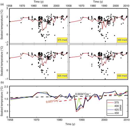
Seabed temperature series for the period 1958–2100 were constructed for each water depth modelled. From 1958 to 2010, we applied an annual interpolation between annually averaged seabed temperatures from oceanographic measurements (Fig. 1). For the rest of the 21st century, we used the rates from the linear temperature trends for the periods 1960–2010 and 1980–2010 of 0.0034°C y⁻¹ and of 0.023°C y⁻¹, respectively (Figs. 2, 5). A rate of 0.023°C y⁻¹ gives a seabed warming of 2.1°C by 2100, about four times larger than the average ocean warming predicted in West Antarctica of 0.5±0.4 by a multi-model ensemble under the A1B scenario (Yin et al. 2011). The observed past temperatures are quite similar for the seabed depth range of our models (Fig. 2), so the linear trends were calculated using average temperatures from the interpolated past temperature series at the four modelled water depths. Future temperatures, starting at 2010, were tied to the mean temperature for the period 2000–2010. Here we implicitly assume that the long-period seabed temperature increase due to ocean warming, that is, the seabed warming trend over the 21st century, is the dominant temperature component controlling the future response of hydrate, as indicated by other hydrate studies in the Arctic (Marín-Moreno et al. 2015). Therefore, we do not consider seabed temperature fluctuations driven by the influence of deep-water undercurrents (e.g., Maldonado et al. 2014) and/or by seasonality (e.g., Meredith et al. 2004; Clarke et al. 2009).

Fig. 2  (a) Seabed temperature data and interpolated temperature series at our study location in the South Shetland Margin for the period 1958–2010 and for 375, 400, 425 and 450 m water depth (mwd). (b) Interpolated temperature series at each water depth and associated temperature trends for the periods 1960–2010 of 0.0034°C y⁻¹, and 1980–2010 of 0.023°C y⁻¹. Note that the temperature trends were estimated using average temperatures from the four water depths modelled.

1D steady-state modelling approach

Steady-state modelling of the evolution of the base of the HSZ assumes: (1) the heat driven by a seabed temperature perturbation has sufficient time to diffuse along the entire HSZ; (2) no hydrate formation or dissociation occurs within the HSZ during that time; and (3) no latent heat. If we accept these assumptions, the validity of which mainly depend on initial thickness of the HSZ, time, sediment thermal diffusivity and hydrate concentration, the “new” steady-state temperature profile is parallel to the initial geothermal gradient, with a positive or negative temperature increment equal to that at the seabed (Fig. 3a). Therefore, for a given seabed temperature perturbation, the intersection between a hydrate stability curve and the “new” steady-state temperature profile gives the depth of the “new” base of the HSZ.

Fig. 3  (a) Comparison between the results obtained at 375 m water depth (mwd) with the steady-state and transient modelling (random distribution, Table 1) approaches for years 1958 (initial conditions) and 2100. The area on the left side of Moridis’ (2003) methane phase boundary for a 3.5% weight total (wt%) salinity contains the pressure and temperature (P–T) conditions for methane hydrate stability. The initial hydrate thickness in both approaches is similar because the transient model is initialized with steady-state conditions. (b) Methane hydrate phase stability boundaries for pure water and 3.5 wt% salinity.

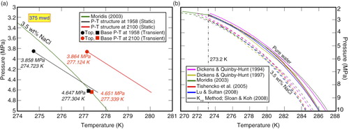
For direct comparison with the results from the transient models (Fig. 3a), we used Moridis’ (2003) methane hydrate stability boundary, a geothermal gradient of 38°C km⁻¹, and converted seabed depth to pressure using a water density of 1046 kg m⁻³ (see Table 1 for comparison with transient model parameters). Moridis’ (2003) stability boundary is defined for pure water; therefore, we applied the relationship put forward by Dickens & Quinby-Hunt (1997) to account for a water salinity of 3.5% weight total (wt%) of sodium chloride. This relation was also applied in Fig. 3b to convert the pure water stability boundary from the distribution coefficient (K_vsi-Value) method (Sloan & Koh 2008) to a 3.5 wt% salinity boundary, and the boundary defined by Dickens & Quinby-Hunt (1994) for 3.35 wt%, to pure water and 3.5 wt% boundaries. For the conversion, we assumed a pure water fusion temperature of 273.2 K, a pure water fusion enthalpy of 6008 J mol⁻¹, an enthalpy of hydrate dissociation of 54 200 J mol⁻¹, six water molecules in the hydrate formula (CH₄·6H2O) and Blangden's law (Ladd 1998) to calculate the fusion temperature of water in an electrolyte solution of 3.5 wt% salinity. For Blangden's law, we assumed a water cryoscopic constant of 1853 K g mol⁻¹ and a sodium chloride van't Hoff factor of 2. The other phase boundaries presented in Fig. 3b are defined for a variable salinity concentration.

Results and discussion

Transient model results show dissociation at the top of the hydrate layer (Fig. 4, Supplementary Fig. S1), and the steady-state model, due to the method's inherent limitation, predicts dissociation of the whole layer (Fig. 3a). It is sometimes assumed that hydrate dissociation starts at the base of the HSZ. However, the initial dissociation zone depends, mainly, on the initial pressure–temperature conditions and the rate of their corresponding changes. At 375 mwd by 2100, the top of the initial hydrate layer is out of its stability field, whereas the base remains stable (Fig. 3a). In an ocean warming scenario, the steady-state modelling approach will always predict the depth of the base of the HSZ shallower or equal to that predicted with the transient. This aspect can be critical when the depth of an observed hydrate-related BSR in deep waters, likely to be in stable conditions, is extrapolated to shallower water depths, where the system may be in a transient state, using the BSR-derived geothermal gradient and the steady-state approach. In the Svalbard continental margin, the error can be as large as 50 ms (Westbrook et al. 2014). An observed deeper hydrate-related BSR compared to the steady-state calculated depth of the base of the HSZ could be attributed to overpressure and/or the presence of other gases, such as ethane, locked in the hydrate (Tinivella & Giustiniani 2013). However, if the in situ pressure and temperature conditions can explain hydrate dissociation, this depth difference could also indicate that the system is in transient state.

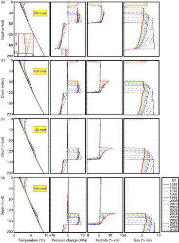
Fig. 4  Results from the random distribution model (Table 1) for a rate of future seabed warming of 0.023°C y⁻¹. Variations in temperature, pressure change (considered as the positive or negative increment in pore water pressure with respect to the initial hydrostatic), hydrate and gas saturations with time and water depth (mwd).

Most hydrate stability boundaries found in the literature do not have a constant pressure–temperature gradient and show a decrease in pressure dependency of the system at deeper waters (Fig. 3b). At relatively shallow waters (below ca. 600 m), the same seabed temperature perturbation generates different hydrate responses at similar water depths (e.g., Marín-Moreno et al. 2015). This behavioural aspect has important implications in polar areas where hydrate is stable in shallow waters. In contrast, the response to seabed warming of a deep-water hydrate reservoir is more uniform and, for a large range of water depths, the modelling of the global behaviour of the system may be reliably performed by a reduced number of 1D transient models.

Over the 21st century, hydrate-sourced methane emissions in the SSM may occur at water depths between 375 and 425 m, if future temperatures follow the trend over the period 1980 to 2010 of 0.023°C y⁻¹ (Fig. 5). For a seabed warming of 0.0034°C y⁻¹, hydrate dissociates at 375 mwd, but the dissociation rate is not sufficient to generate seabed emissions during the 21st century. The results obtained using the 0.023°C y⁻¹ seabed warming scenario are discussed below.

Fig. 5  Past (solid lines) and future (thick black dashed lines) seabed temperatures for the period 1958–2100. Associated seabed methane emissions calculated using the uniform (dashed lines) and random (dashed-point lines) distribution models (Table 1) for the 0.023°C y⁻¹ future temperature trend. Note that seabed methane emissions do not occur at 450 m water depth (mwd) when using the 0.023°C y⁻¹ temperature trend, and at any water depth for the 0.0034°C y⁻¹ trend.

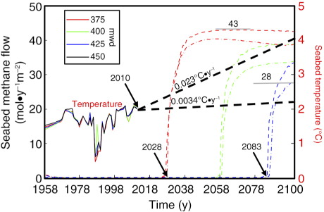
At 375 mwd, hydrate-sourced methane emissions would start at ca. 2028 and may extend to deeper waters at an average rate of 0.91 mwd y⁻¹ (Fig. 6). The rate of hydrate-sourced methane transport to the seabed for the uniform model (Table 1) ranges between 43 and 33 mol y⁻¹ m⁻² (Fig. 5) and is controlled by the rate at which heat is supplied to the system (Thatcher et al. 2013). The heat supplied to a hydrate system is consumed first to move the temperature of the system towards its phase boundary and then to overcome the latent heat of dissociation (until all the hydrate dissociates). For the same initial seabed temperature, seabed heat supply and hydrate saturation, at deeper water depths dissociation affects a thinner hydrate thickness (Fig. 4), and so the methane generation rate and associated seabed emissions decrease (Fig. 5). Both distributions of hydrate and free gas show similar seabed methane emissions (Fig. 5), though emissions from the uniform distribution model are slightly higher because of its higher initial hydrate saturation (Table 1). Results from the random distribution model (Table 1) show that a significant amount of the free methane flowing upwards from the free gas layer can reform hydrate when it enters the HSZ, which acts as a methane capacitor (Dickens 2011; Fig. 4). Some of the free methane can overpass the HSZ filter and, by the end of the 21st century, start to contribute to the total methane outflow by increasing the methane concentration close to the seabed (Fig. 4a). This free methane inflow will probably increase the seabed methane outflow beyond 2100.

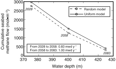
Fig. 6  Cumulative seabed methane emissions by 2100 calculated at 375, 400 and 425 m water depth (mwd) for the random (dashed line) and uniform (solid line) distribution models (Table 1). The number below each circle indicates the time of the first seabed methane emission and the inset the propagation rate of methane emissions with water depth. The area under the curves gives the total methane released at the seabed per metre along the margin for the period 2028–2100.

Overpressure (pore pressure above hydrostatic) generation by hydrate dissociation is governed by the balance between the rates of hydrate dissociation and pressure dissipation (Holtzman & Juanes 2011), and it is associated with submarine geohazards including fractures and liquefaction (Xu & Germanovich 2006) and landslides (Sultan et al. 2004; Xu & Germanovich 2006). Overpressure-induced slope failure can be explained by a 1D analysis of the factor of safety (FS) of an infinite slope (e.g., Lambe & Whitman 1969; Eqn. 1). It occurs when the failure-inducing stress, that is, the weight component in the direction of the slope, exceeds the shear strength of the sediment, given by the Mohr-Coulomb failure criterion (FS<1). This approach assumes a parallel failure plane to the seafloor and a much thinner failure in depth than in the longitudinal axes, and neglects edge effects.1

In Eqn. 1, FS is factor of safety, is cohesion, is vertical stress, P _h is hydrostatic pore pressure, P* is overpressure, θ is slope and is friction angle. The generation of vertical hydrofractures can be conservatively estimated when the overpressure exceeds the horizontal effective stress (Aldridge & Haland 1991). We implicitly assume that the maximum principal effective stress is vertical and the intermediate and minimum principal effective stresses are horizontal (e.g., Daigle & Dugan 2010). Here we analyse the likelihood of shallow landslides and vertical fractures to occur in the SSM caused only by hydrate dissociation-induced overpressure over the 21st century. We consider the following parameters: (1) a of 25°; (2) shallow normally consolidated sediments with a of ca. 0 (Lambe & Whitman 1969) and with a ratio between the maximum-vertical to the minimum-horizontal effective stress (K ₀), as given by Jaky's equation (; Jaky 1948) of 0.58; (3) a slope of 1° (estimated in the SSM for a seabed depth range from 375 to 450 m); (4) the water and grain densities, and porosity function as given in Table 1; and (5) an overpressure generated from hydrate dissociation at 375 mwd of 6 KPa (Fig. 4a). We estimate a ratio of overpressure to vertical effective stress in hydrostatic conditions (λ*) of 0.54 and a FS of 12 at 2 m below seafloor (mbsf), and of 0.21 and 21, respectively, at 5 mbsf. Even at a shallow depth of 2 mbsf, λ* is slightly lower than the K ₀ and the FS is significantly higher than one. This indicates that shallow hydrofracturing and slope failure due to hydrate dissociation-generated overpressure is unlikely in the SSM over the 21st century. This result agrees with the pore-scale modelling result of Holtzman & Juanes (2011) in which, generally, the timescale of pore pressure build-up by hydrate dissociation is much larger than its dissipation. However, the calculated overpressure is controlled by our assumed high intrinsic permeability of 10⁻¹³ m² (Table 1). Thatcher et al. (2013) shows that using a similar rate of seabed warming and hydrate saturation, and an intrinsic permeability of 10⁻¹⁶ m² the pore pressure excess the lithostatic load only a few years after hydrate starts to dissociate.

In the SSM and if the rate of seabed temperature increase follows the trend over the period 1980–2010, we estimate a depth range of potential hydrate-sourced methane emissions between 375 and 442 mwd (here we have applied a propagation rate of the emissions with water depth of 1 mwd y⁻¹ from 2083 to 2100; Fig. 6). For this depth range and for the period 2028–2100, the potential amount of dissociated methane liberated to the ocean may be between 1.06 and 1.21×10³ mol y⁻¹ per metre along the margin for the random and uniform distribution models, respectively (Fig. 6). Our calculated hydrate-sourced methane emissions in the SSM are similar to those per metre along the continental margin west of Svalbard of 0.4–4.5×10³ mol y⁻¹, estimated using a bubble catcher and video in 2012 (Sahling et al. 2014), and lower than those modelled and 21st century-averaged of 2.4–25.7×10³ mol y⁻¹ (Marín-Moreno et al. 2015). In polar areas, 21st century-averaged hydrate-sourced emissions are greater than present-day emissions because the ocean temperature generally increases and hence the area of potential emissions extends. Over the 21st century, the total amount of hydrate-sourced methane emitted to the ocean per metre along the SSM may be about an order of magnitude smaller than that from the continental margin west of Svalbard.

In a global context of carbon emissions to the ocean and atmosphere, 21st century hydrate-sourced methane emissions are a minor player (Marín-Moreno et al. 2015). However, the identification and study of key areas likely to experience the effects of warming-induced hydrate dissociation is essential to observe and understand the long-term evolution (centennial to millennial time scales) of a natural compound that may be linked to past abrupt climate change events (e.g., Dickens 2011).

Conclusions

From the results of the transient modelling of ocean warming-induced hydrate dissociation in the SSM, we conclude that over the 21st century, hydrate-sourced methane emissions may occur at water depths between 375 and 425 m if the future seabed temperatures follow a similar trend to that over the period 1980 to 2010 of 0.023°C y⁻¹. Emissions would not occur with a seabed warming rate an order of magnitude smaller. Hydrate dissociation would initiate at the top of the hydrate layer, and the overpressure generated would not be sufficient to cause, by itself, shallow slope failures or shallow vertical fractures over the 21st century. Hydrate-sourced methane emissions at 375 mwd would start at ca. 2028 and may extend to deeper waters at an average rate of 0.91 mwd y⁻¹. Over the 21st century, the potential amount of dissociated methane liberated to the ocean may be between 1.06 and 1.21×10³ mol y⁻¹ per metre along the margin, an order of magnitude smaller than that from the Arctic continental margin west of Svalbard. The SSM is one of the key areas to observe and understand the effects of warming-induced hydrate dissociation in the Southern Hemisphere during the coming decades.

From the results and general comparison of the steady-state and transient modelling approaches, we conclude that steady-state modelling of the thickness of the HSZ beneath the seabed should be applied only to stable hydrate systems. Under an ocean warming scenario in which dissociation may occur, it provides an upper bound of the potential hydrate-sourced methane that could be liberated to the ocean. Depending on the initial pressure–temperature conditions and the magnitude of their corresponding perturbations, in transient conditions dissociation can initiate at the top of the hydrate layer, a mechanism that the steady-state approach cannot represent. In a hydrate system where the in situ pressure and temperature conditions indicate hydrate dissociation, a depth difference between an observed hydrate-related BSR and the steady-state calculated base of the HSZ could be explained by a transient state of the system.

Acknowledgements

This work was partly supported by the TALENTS FVG Programme—Activity 1—Incoming Mobility Scheme—European Social Fund, Operational Programme 2007—2013, Objective 2 Regional Competitiveness and Employment, Axis 5 Transnational cooperation. This work was also partially supported by the Ministry of Education, Universities and Research under the grant for Italian participation in the activities related to the international infrastructure Partnership for Advanced Computing in Europe. We thank the National Oceanic and Atmospheric Administration National Oceanographic Data Center (www.nodc.noaa.gov/cgi-bin/OC5/WOA09/woa09.pl) for making available the ocean temperature data, the International Bathymetric Chart of the Southern Ocean project (www.ibcso.org/data.html) for the bathymetric data and the Global Heat Flow Database of the International Heat Flow Commission (www.heatflow.und.edu/index2.html) for the thermal conductivity data. We also thank Luis Somoza and an anonymous reviewer for their constructive comments.

References

- Aldridge T.R., Haland G. Assessment of conductor setting depth. Paper presented at the 23rd Annual Offshore Technology Conference. 1991; TX: Houston.
- Arndt J.E., Schenke H.W., Jakobsson M., Nitsche F., Buys G., Goleby B., Rebesco M., Bohoyo F., Hong J.K., Black J., Greku R., Udintsev G., Barrios F., Reynoso-Peralta W., Morishita T., Wigley R. The International Bathymetric Chart of the Southern Ocean (IBCSO) version 1.0—a new bathymetric compilation covering circum-Antarctic waters. Geophysical Research Letters. 2013; 40: 3111–3117.
- Barker P.F., Kennett J.P., Shipboard Scientific Party . Proceedings ODP. Initial Reports 113. 1988; College Station, TX: Ocean Drilling Program.
- Boetius A., Wenzhöfer F. Seafloor oxygen consumption fuelled by methane from cold seeps. Nature Geoscience. 2013; 6: 725–734.
- Buffett B., Archer D. Global inventory of methane clathrate: sensitivity to changes in the deep ocean. Earth and Planetary Science Letters. 2004; 227: 185–199.
- Chapman W.L., Walsh J.E. A synthesis of Antarctic temperatures. Journal of Climate. 2007; 20: 4096–4117.
- Clarke A., Griffiths H.J., Barnes D.K.A., Meredith M.P., Grant S.M. Spatial variation in seabed temperatures in the Southern Ocean: implications for benthic ecology and biogeography. Journal of Geophysical Research—Biogeosciences. 2009; 114: 03003. http://dx.doi.org/10.1029/2008jg000886.
- Dai S., Santamarina J.C. Water retention curve for hydrate-bearing sediments. Geophysical Research Letters. 2013; 40: 5637–5641.
- Dai S., Seol Y. Water permeability in hydrate-bearing sediments: a pore-scale study. Geophysical Research Letters. 2014; 41: 4176–4184.
- Daigle H., Dugan B. Origin and evolution of fracture-hosted methane hydrate deposits. Journal of Geophysical Research—Solid Earth. 2010; 115: 11101–11121.
- Dickens G.R. Down the rabbit hole: toward appropriate discussion of methane release from gas hydrate systems during the Paleocene–Eocene thermal maximum and other past hyperthermal events. Climate of the Past. 2011; 7: 831–846.
- Dickens G.R., Quinby-Hunt M.S. Methane hydrate stability in seawater. Geophysical Research Letters. 1994; 21: 2115–2118.
- Dickens G.R., Quinby-Hunt M.S. Methane hydrate stability in pore water: a simple theoretical approach for geophysical applications. Journal of Geophysical Research—Solid Earth. 1997; 102: 773–783.
- Giustiniani M., Accettella A., Loreto M., Tinivella U., Accaino F. Geographic information system—an application to manage geophysical data. Proceedings of the 71st European Association of Geoscientists and Engineers Conference and Exhibition. Vol. 1. 2009; Amsterdam: Society of Petroleum Engineers. 340–344.
- Holtzman R., Juanes R. Thermodynamic and hydrodynamic constraints on overpressure caused by hydrate dissociation: a pore-scale model. Geophysical Research Letters. 2011; 38: 14308. http://dx.doi.org/10.1029/2011gl047937.
- Hunter S.J., Goldobin D.S., Haywood A.M., Ridgwell A., Rees J.G. Sensitivity of the global submarine hydrate inventory to scenarios of future climate change. Earth and Planetary Science Letters. 2013; 367: 105–115.
- Jaky J. Pressure in silos. Proceedings of the Second International Conference on Soil Mechanics and Foundation Engineering. Vol. 1. 1948; Rotterdam: International Conference on Soil Mechanics and Foundation Engineering. 103–107.
- Ladd M. Introduction to physical chemistry. 1998; Cambridge: Cambridge University Press.
- Lambe T.W., Whitman R.V. Soil mechanics. 1969; New York: Wiley.
- Liu X., Flemings P.B. Dynamic multiphase flow model of hydrate formation in marine sediments. Journal of Geophysical Research—Solid Earth. 2007; 112: 03212. http://dx.doi.org/10.1029/2005JB004227.
- Lodolo E., Camerlenghi A., Brancolini G. A bottom simulating reflector on the South Shetland margin, Antarctic Peninsula. Antarctic Science. 1993; 5: 207–210.
- Lodolo E., Camerlenghi A., Madrussani G., Tinivella U., Rossi G. Assessment of gas hydrate and free gas distribution on the South Shetland margin (Antarctica) based on multichannel seismic reflection data. Geophysical Journal International. 2002; 148: 103–119.
- Loreto M.F., Tinivella U. Gas hydrate versus geological features: the South Shetland case study. Marine and Petroleum Geology. 2012; 36: 164–171.
- Lu Z., Sultan N. Empirical expressions for gas hydrate stability law, its volume fraction and mass-density at temperatures 273.15 K to 290.15 K. Geochemical Journal. 2008; 42: 163–175.
- Maldonado A., Bohoyo F., Galindo-Zaldívar J., Hernández-Molina F.J., Lobo F.J., Lodolo E., Martos Y.M., Pérez L.F., Schreider A.A., Somoza L. A model of oceanic development by ridge jumping: opening of the Scotia Sea. Global and Planetary Change 123 Part B. 2014; 152–173.
- Marín-Moreno H., Minshull T.A., Westbrook G.K., Sinha B. Estimates of future warming-induced methane emissions from hydrate offshore west Svalbard for a range of climate models. Geochemistry, Geophysics, Geosystems. 2015; 16: 1307–1323.
- Marín-Moreno H., Minshull T.A., Westbrook G.K., Sinha B., Sarkar S. The response of methane hydrate beneath the seabed offshore Svalbard to ocean warming during the next three centuries. Geophysical Research Letters. 2013; 40: 4977–5336.
- Meredith M.P., Renfrew I.A., Clarke A., King J.C., Brandon M.A. Impact of the 1997/98 ENSO on upper ocean characteristics in Marguerite Bay, western Antarctic Peninsula. Journal of Geophysical Research—Oceans. 2004; 109: 09013. http://dx.doi.org/10.1029/2003jc001784.
- Moridis G. Numerical studies of gas production from methane hydrates. SPE Journal. 2003; 8: 359–370.
- Moridis G.J., Kowalsky M.B., Pruess K. TOUGH+HYDRATE v1.2 user's manual: a code for the simulation of system behavior in hydrate-bearing geological media. 2012; Berkeley, CA: Lawrence Berkeley National Laboratory, University of California.
- Moridis G.J., Seol Y., Kneafsey T. Studies of reaction kinetics of methane hydrate dissociation in porous media. Proceedings of the 5th International Conference on Gas Hydrates 2005. Vol. 1. 2005; Trondheim: Tapir Academic Press. 21–30.
- Mulvaney R., Abram N.J., Hindmarsh R.C., Arrowsmith C., Fleet L., Triest J., Sime L.C., Alemany O., Foord S. Recent Antarctic Peninsula warming relative to Holocene climate and ice-shelf history. Nature. 2012; 489: 141–144. [PubMed Abstract].
- Neagu R.C., Tinivella U., Volpi V., Rebesco M., Camerlenghi A. Estimation of biogenic silica contents in marine sediments using seismic and well log data: Sediment Drift 7, Antarctica. International Journal of Earth Sciences. 2009; 98: 839–848.
- Reagan M.T., Moridis G.J., Elliott S.M., Maltrud M. Contribution of oceanic gas hydrate dissociation to the formation of Arctic Ocean methane plumes. Journal of Geophysical Research—Oceans. 2011; 116: 09014. http://dx.doi.org/10.1029/2011JC007189.
- Sahling H., Römer M., Pape T., Bergès B., dos Santos Fereirra C., Boelmann J., Geprägs P., Tomczyk M., Nowald N., Dimmler W., Schroedter L., Glockzin M., Bohrmann G. Gas emissions at the continental margin west of Svalbard: mapping, sampling, and quantification. Biogeosciences. 2014; 11: 6029–6046.
- Shipley T.H., Houston M.H., Buffler R.T., Shaub F.J., McMillen K.J., Ladd J.W., Worzel J.L. Seismic evidence for widespread possible gas hydrate horizons on continental slopes and rises. American Association of Petroleum Geologists Bulletin. 1979; 63: 2204–2213.
- Sloan E.D., Koh C. Clathrate hydrates of natural gases. 2008; 3rd edn, Boca Raton, FL: CRC Press.
- Somoza L., León R., Medialdea T., Pérez L.F., González F.J., Maldonado A. Seafloor mounds, craters and depressions linked to seismic chimneys breaching fossilized diagenetic bottom simulating reflectors in the central and southern Scotia Sea, Antarctica. Global and Planetary Change 123 Part B. 2014; 359–373.
- Stone H. Probability model for estimating three-phase relative permeability. Journal of Petroleum Technology. 1970; 22: 214–218.
- Sultan N., Cochonat P., Foucher J.-P., Mienert J. Effect of gas hydrates melting on seafloor slope instability. Marine Geology. 2004; 213: 379–401.
- Thatcher K.E., Westbrook G.K., Sarkar S., Minshull T.A. Methane release from warming-induced hydrate dissociation in the west Svalbard continental margin: timing, rates, and geological controls. Journal of Geophysical Research—Solid Earth. 2013; 118: 22–38.
- Tinivella U. A method for estimating gas hydrate and free gas concentrations in marine sediments. Bollettino di Geofisica Teorica ed Applicata. 1999; 40: 19–30.
- Tinivella U., Accaino F. Compressional velocity structure and Poisson's ratio in marine sediments with gas hydrate and free gas by inversion of reflected and refracted seismic data (South Shetland Islands, Antarctica). Marine Geology. 2000; 164: 13–27.
- Tinivella U., Accaino F., Della Vedova B. Gas hydrates and active mud volcanism on the South Shetland continental margin, Antarctic Peninsula. Geo-Marine Letters. 2008; 28: 97–106.
- Tinivella U., Giustiniani M. Variations in BSR depth due to gas hydrate stability versus pore pressure. Global and Planetary Change. 2013; 100: 119–128.
- Tinivella U., Giustiniani M., Accettella D. BSR versus climate change and slides. Journal of Geological Research 2011. 2011. article no. 390547, doi: http://dx.doi.org/10.1155/2011/390547.
- Tinivella U., Loreto M.F., Accaino F. Regional versus detailed velocity analysis to quantify hydrate and free gas in marine sediments: the South Shetland Margin case study, Geological Society. London, Special Publications. 2009; 319: 103–119.
- Tishchenko P., Hensen C., Wallmann K., Wong C.S. Calculation of the stability and solubility of methane hydrate in seawater. Chemical Geology. 2005; 219: 37–52.
- van Genuchten M.T. A closed-form equation for predicting the hydraulic conductivity of unsaturated soils. Soil Science Society of America Journal. 1980; 44: 892–898.
- Vaughan D.G., Marshall G.J., Connolley W.M., Parkinson C., Mulvaney R., Hodgson D.A., King J.C., Pudsey C.J., Turner J. Recent rapid regional climate warming on the Antarctic Peninsula. Climatic Change. 2003; 60: 243–274.
- Volpi V., Camerlenghi A., Hillenbrand C.D., Rebesco M., Ivaldi R. Effects of biogenic silica on sediment compaction and slope stability on the Pacific margin of the Antarctic Peninsula. Basin Research. 2003; 15: 339–363.
- Westbrook G.K., Minshull T.A., Ker S., Marset B., Sarkar S., Marín-Moreno H., Sinha B. Hydrate beneath the seabed offshore Svalbard, indirect evidence from seismic surveys and thermal modelling. 2014; Russia: St. Petersburg. Paper presented at the Minerals of the Ocean-7 & Deep-Sea Minerals and Mining-4 International Conference. 2–6 June.
- Westbrook G.K., Thatcher K.E., Rohling E.J., Piotrowski A.M., Pälike H., Osborne A.H., Nisbet E.G., Minshull T.A., Lanoisellé M., James R.H., Huhnerbach V., Green D., Fisher R.E., Crocker A.J., Chabert A., Bolton C., Beszczynska-Möller A., Berndt C., Aquilina A. Escape of methane gas from the seabed along the west Spitsbergen continental margin. Geophysical Research Letters. 2009; 36: 15608. http://dx.doi.org/10.1029/2009GL039191.
- Xu T., Ontoy Y., Molling P., Spycher N., Parini M., Pruess K. Reactive transport modeling of injection well scaling and acidizing at Tiwi field, Philippines. Geothermics. 2004; 33: 477–491.
- Xu W., Germanovich L.N. Excess pore pressure resulting from methane hydrate dissociation in marine sediments: a theoretical approach. Journal of Geophysical Research—Solid Earth. 2006; 111: 01104. http://dx.doi.org/10.1029/2004jb003600.
- Yin J., Overpeck J.T., Griffies S.M., Hu A., Russell J.L., Stouffer R.J. Different magnitudes of projected subsurface ocean warming around Greenland and Antarctica. Nature Geosciences. 2011; 4: 524–528.