
Abstract
A lithological and foraminiferal study of newly acquired sediment cores outside the Ingøydjupet (Ingøy Deep) trough has been carried out to improve constraints on the last deglacial history in the south-western Barents Sea. Three lithofacies and three foraminiferal facies were identified. The lowermost lithological unit is a diamicton interpreted as glacial till. It contains a low-abundance, ecologically mixed foraminiferal assemblage, presumably resulting from glacial reworking. Above the diamicton, a layer of ice-rafted debris (IRD), likely associated with intensive iceberg production, marks the initial destabilization of the marine-based ice sheet. At this time, ca. 15.6–15.0 Ky B.P., opportunistic foraminiferal species Nonionellina labradorica and Stainforthia spp. reached peak abundance. During the south-western Barents Sea ice-margin retreat, presumably corresponding to the Bølling interstadial, a sequence of glaciomarine laminations was deposited conformably on the layer of IRD. Sedimentation rates were apparently high (estimated about 0.4 cm per year) and the foraminiferal fauna was dominated by Elphidium spp. and Cassidulina reniforme, species common for glacier-proximal environments. A hiatus at the top of the deglacial unit is likely linked to the high bottom-current activity associated with a strengthened inflow of Atlantic water masses into the Barents Sea. The uppermost lithological unit is represented by the Holocene marine sandy mud. It contains a high-abundance, high-diversity foraminiferal fauna with common cassidulinids, Cibicides spp., Epistominella pusilla and planktic species.
To access the supplementary material for this article, please see the supplementary file under Article Tools, online.
Increasing attention has been paid over the past decade to the dynamics of marine-based ice sheets, which are ice sheets grounded below sea level (e.g., Grosfeld & Sandhäger Citation2004; Svendsen et al. Citation2004; Heroy & Anderson Citation2007; Smith et al. Citation2011; Bigg et al. Citation2012; Hillenbrand et al. Citation2012). Interest stems from the fact that these bodies of ice are inherently unstable; a minor retreat could trigger a destabilization of the entire ice sheet, leading to its collapse (e.g., Hughes Citation2011). Two major examples of late Quaternary marine-based ice sheets are the Barents–Kara and the West Antarctic ice sheets. At present, collapse of the West Antarctic ice sheet threatens to increase global sea levels (Joughin & Alley Citation2011 and references therein). In addition, understanding the behaviour of the Greenlandic marine-terminating glaciers is of importance for the assessment of future sea level (Nick et al. Citation2009). Insights into the dynamics of these modern marine-terminating ice margins can be gained by using the palaeo-ice sheet that covered the Barents and Kara seas as an analogue (Ingólfsson & Landvik Citation2013).
Abbreviations in this article
CT: computerized tomography
IRD: ice-rafted debris
Ky B.P.: thousand calendar years before 1950
MS: magnetic susceptibility
SEM-EDS: scanning electron microscopy with energy-dispersive x-ray spectroscopy
SI: International System of Units
Several studies addressed the issue of defining the extent and timing of the ice sheet in the Barents Sea region during Late Weichselian time (e.g., Elverhøi et al. Citation1993; Lambeck Citation1996; Landvik et al. Citation1998; Ottesen et al. Citation2001; Olsen Citation2002; Ottesen et al. Citation2005; Sejrup et al. Citation2005). There is a general agreement that the ice sheet extended to the shelf break along the western Barents Sea margin () at least twice: before 22 Ky B.P. and after 19 Ky B.P. (Vorren & Laberg Citation1996). The ice-sheet margin then retreated rapidly by iceberg calving within the deeper troughs, which served as outlets for fast-flowing ice streams (Vorren & Laberg Citation1996; Landvik et al. Citation1998). The deglaciation was coeval with rising sea level (Clark et al. Citation2009) and was greatly influenced by the influx of Atlantic water masses (e.g., Chistyakova et al. Citation2010; Junttila et al. Citation2010). It was, however, punctuated by periods of ice margin stability and readvances, as evidenced by a series of ice-marginal deposits (Andreassen et al. Citation2008; Ottesen et al. Citation2008; Winsborrow et al. Citation2010). The rates of retreat were particularly high in Bjørnøyrenna (Bear Island Trough), the largest trough in the western Barents Sea (), where Winsborrow et al. (Citation2010) estimate retreat rates of 60–275 m year−1. By 16 Ky B.P., Bjørnøyrenna was almost entirely ice-free, while by 15 Ky B.P. the ice-sheet margin had retreated onshore in all areas of the western Barents Sea (Winsborrow et al. Citation2010). This made ice loss by calving no longer possible, and the rate of retreat slowed significantly (Winsborrow et al. Citation2010).
Fig. 1 Regional bathymetry of the south-western Barents Sea, showing the main troughs and banks (Andreassen et al. Citation2008). Also indicated are the approximate locations of the cores used in the present and previous studies. Bathymetry from the Norwegian Hydrographic Service (www.mareano.no).
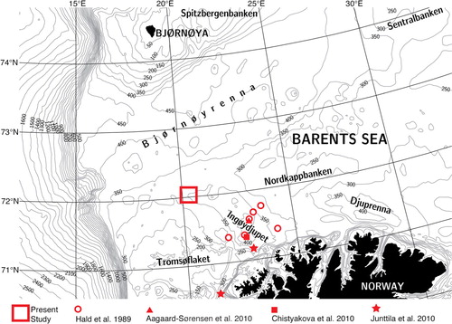
The focus of this article is on the last deglaciation of the south-western sector of the Barents Sea shelf (). The glacigenic sediments in this region have been investigated mainly with the aid of two- and three-dimensional seismic data, sub-bottom profiling and/or multibeam bathymetry (Vorren & Kristoffersen Citation1986; Vorren et al. Citation1990; Andreassen et al. Citation2008; Bellec et al. Citation2008; Ottesen et al. Citation2008; Winsborrow et al. Citation2010; Rebesco et al. Citation2011; Rüther et al. Citation2011; Bjarnadóttir et al. Citation2012). The studies based on the analysis of sediment cores (Hald et al. Citation1989; Ivanova et al. Citation2002; Aagaard-Sørensen et al. Citation2010; Chistyakova et al. Citation2010; Junttila et al. Citation2010) have focused on sites of high sedimentation rate such as the Ingøydjupet (Ingøy Deep) trough (). The present work provides new sediment-core data from the area just outside Ingøydjupet to better constrain the history of the last deglaciation in the south-western Barents Sea at shallower water depths. The specific objectives were to (1) identify major lithofacies, (2) distinguish foraminiferal assemblage zones and (3) reconstruct sedimentary environments during and after the last deglaciation. By combining x-ray tomography, gamma density, MS, grain size analysis, SEM-EDS, biostratigraphy and radiocarbon dating, this study could hold promise for improving constraints on deglacial events in other areas of the Barents Sea via stratigraphic correlation.
Data and methods
Multibeam swath bathymetry of the study area () was acquired by the Norwegian Defence Research Establishment in 2009 with a Kongsberg Maritime EM710 multibeam echosounder. The data have a resolution of 1–2 m and 0.1–0.2 m in the horizontal and vertical directions, respectively.
Fig. 2 Bathymetry of the study area with the coring sites. See for location in the south-western Barents Sea. Note the occurrence of several pockmarks, appearing as circular depressions (Pau et al. Citation2014). Multibeam bathymetry acquired by the Norwegian Defence Research Establishment.
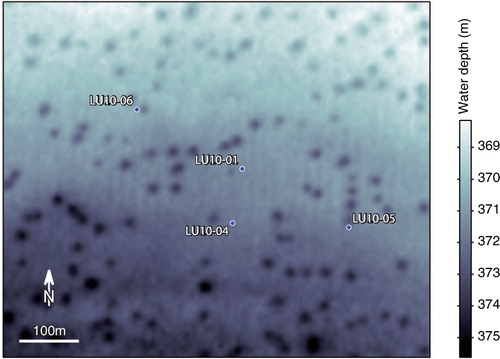
Four gravity cores (, ) were collected with the Norwegian Defence Research Establishment's RV H.U. Sverdrup II in 2010. The cores are each 60 mm in diameter and were sampled outside of pockmarks. Recovery ranged from 142 to 165 cm. Accurate locations of the coring sites were recorded using a hydroacoustic position reference system.
Table 1 Length, water depth and position (WGS84) of the Lundin Petroleum 2010 (LU10) cores.
Lithological analyses included x-ray tomography, gamma density and MS measured with a multi-sensor core logger, coarse grain size (, ), as well as SEM-EDS (Supplementary Fig. S1).
Fig. 3 CT image, lithological units (dashed lines) and subunits (dotted lines), x-ray and gamma density, MS and grain size (gravel, >2000 µm; sand, 63–2000 µm) for the investigated cores. Average ages (Ky B.P.) of the dated intervals are indicated. Details of the CT images are illustrated in .
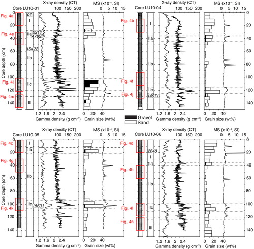
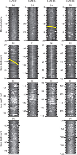
Fig. 4 Detailed views of the CT images: (a–d) Holocene marine sediments (Lithological Unit I); (e–h) glaciomarine laminated sediments (Lithological Unit II, Subunit IIb); (i–l) IRD layer (Lithological Unit II, Subunit IIc); (m) and (n) glacial till (Lithological Unit III). Columns from left to right refer to cores LU10-01, LU10-04, LU10-05 and LU10-06. The yellow line in (c) marks the contact between Lithological Unit I and the IRD layer topping Lithological Unit II (Subunit IIa), while in (e) it marks the erosion surface between Subunit IIa and the underlying laminations (Subunit IIb).
X-ray tomography was carried out with a Siemens Somatom whole-body CT scanner at the Norwegian University of Life Sciences in Ås, Norway, at a resolution of 1 mm. X-ray density estimated after Boespflug et al. (Citation1995) is expressed in CT numbers averaged over the 40 central pixels of the image with a 3-point running average.
After splitting, the cores were scanned for gamma ray attenuation and MS (given following SI conventions) at the Department of Earth Science, University of Bergen, Norway, at a resolution of 1 cm.
Grain size analyses were performed on 5-cm-long sections. The samples were freeze–dried, weighed and wet-sieved at 63 µm. The coarser fraction was dried in an oven at 40°C and sieved at 2000 µm. The relative content of gravel (>2000 µm) and sand (63–2000 µm) is given as a dry weight percentage of the total sample weight.
SEM-EDS was performed on a limited number of samples in core LU10-06 at the Natural History Museum of the University of Oslo, Norway, in order to investigate the nature of some particles suspected to have ferrimagnetic behaviour.
The total number of foraminifera per unit weight of dry sediment was evaluated in core LU10-01 (), while the remaining cores were used to estimate relative abundances (, ). Benthic foraminifera were counted in the >63 µm fraction for every 5-cm slice of the cores. The fine mesh was used in order not to miss small specimens. However, most of the identified foraminifera are larger than 100 µm, meaning that our results can be compared with those of other studies using larger meshes. The only exception is Epistominella pusilla (see taxonomical note and Supplementary Fig. S2 in the Supplementary File), which has a large variation in size including some very small specimens. Therefore, previous articles using 100 or 125 µm sieve size may have underestimated its abundance slightly. However, Risebrobakken et al. (Citation2010) and Chistyakova et al. (Citation2010), using 100 µm sieve size, counted E. pusilla up to 40 and 57%, respectively, in the upper part of their Barents Sea cores, similar to our numbers. Whenever possible, 300 specimens were counted, but in low-abundance samples smaller counts were accepted. Relative abundances of the most abundant and/or stratigraphically informative taxa are reported as percentages of the total fauna (). A simplified taxonomy was used with 25 taxa identified mainly to the species and genus level. Specimens of Elphidium were counted as a genus, although several species were probably present. An exception was made for the distinct, often very large form E. bartletti. Cassidulinids were mostly counted on the family level, but with Cassidulina reniforme identified as a separate taxon. The relative abundances of C. neoteretis and Islandiella spp. were noted qualitatively. Minor taxa not presented here include Pullenia bulloides, Fissurina sp., Lagena spp. (mainly L. distoma), Uvigerina sp., Lenticulina sp. and Bulimina marginata (in some core-bottom samples). Most of these taxa were found only in the Assemblage Zone A (see below), but Lagena spp. also occurred in Zone C. Bulimina marginata was found only in Zone C.
Fig. 5 Total number of foraminiferal specimens per unit weight of dry sediment (histogram) in core LU10-01. Assemblage Zones A, B and C (shades of grey), Lithological Units I, II and III (dashed lines) and Lithological Subunits IIa, IIb and IIc (dotted lines) are marked.
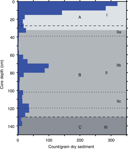
Fig. 6 Frequency distribution (%) of the main benthic foraminiferal taxa and the total planktic fauna in the >63 µm fraction in the studied cores. Assemblage Zones A, B and C (shades of grey), Lithological Units I, II and III (dashed lines) and Lithological Subunits IIa, IIb and IIc (dotted lines) are marked. Ages (Ky B.P.) are also indicated.
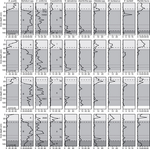
Fig. 7 Relative abundances of planktic foraminifera in core LU10-06 (percentages of the total planktic fauna). Assemblage Zones A, B and C (shades of grey), Lithological Units I, II and III (dashed lines) and Lithological Subunits IIa, IIb and IIc (dotted lines) are marked.
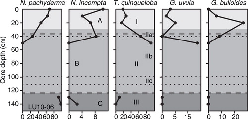
Planktic foraminifera were also counted in the >63 µm fraction. Since they were scarce, we merged pairs of samples to obtain acceptable sample sizes (n>30), giving 10-cm vertical resolution. The following forms were counted in core LU10-06 (): Neogloboquadrina pachyderma, N. incompta, Turborotalita quinqueloba, Globigerinita uvula and Globigerina bulloides. Other species of planktic foraminifera were very rare. Studies using 100 or 125 µm sieve size may have underestimated the abundance of the relatively small species T. quinqueloba and G. uvula.
The biostratigraphic divisions were validated by clustering the foraminiferal assemblages (Supplementary Fig. S3) using stratigraphically constrained unweighted pair group method with arithmetic mean with the Bray–Curtis distance measure, in PAST ver. 3.0 (Hammer et al. Citation2001).
Seven 14C radiocarbon dates () were obtained from macroscopic shell material and collections of foraminifera. The analyses were carried out by means of accelerator mass spectrometry at the Radiocarbon Dating Laboratory of Lund University, Sweden. The radiocarbon dates were calibrated using the Calib v. 7.0 software (Stuiver & Reimer Citation2014) with the Marine13 calibration curve (Reimer et al. Citation2013), which operates with a standard reservoir correction of 400 years (ΔR=0). The employed total reservoir age was 467±41 years (ΔR=67±41), which is considered representative for the waters off northern Norway (Mangerud & Gulliksen Citation1975; Reimer & Reimer Citation2001).
Table 2 Results from accelerator mass spectrometry 14C radiocarbon dating and calendar (cal.) year calibrations. The error in 14C age (not reservoir corrected) is given as ±1σ. The analyses were conducted at the Radiocarbon Dating Laboratory, Lund University, Sweden. The dates were calibrated into calendar years before 1950 (years B.P.) using the Marine13 calibration curve (Reimer et al. Citation2013) and are given as 95% confidence intervals. A standard reservoir correction of 400 years with an additional reservoir correction ΔR=67±41 was employed.
Results
Visually, the sediments appeared as grey mud for most part of the cores, with the top 10–20 cm often showing a brownish colour. The top 1 cm was rich in sponge spicules. Gravel particles were occasionally visible and were interpreted as iceberg dropstones. Almost no well-preserved macroscopic shells were encountered.
Inspection of the CT images revealed significant details of the internal structure of the cores (, ) and provided the basis to identify the lithological units described below. The x-ray and gamma density logs were rather consistent with each other (), with density slightly increasing downcore as a result of sediment consolidation. Because of variation in the thickness of the split cores, however, the calibrated gamma density values are not considered to be fully reliable. MS () is controlled by density and mineralogy; local variations may therefore be influenced by the content of sand and gravel minerals, which possess higher values than clay minerals, and by authigenic formation of ferrimagnetic minerals.
Lithostratigraphy
Three lithological units are distinguished based on the CT images, and with the support of the density, grain size and MS logs (, ).
Lithological Unit III. This unit is observed at the bottom 20–30 cm of cores LU10-01 and LU10-06. The unit appears in the CT images as a diamicton (, m–n). The coarsest fraction is composed of rounded to angular particles, typically 2–3 cm in size (m–n). Sand content is around 15%, while MS values are generally lower than 2×10⁻⁴ ().
Lithological Unit II. Near the bottom of the unit, a 10-cm-thick layer (Subunit IIc) is observed with the brightest intensity in the CT images. Its depth varies from 98 to 123 cm in the different cores (i–l). This layer is dated to 15.6 Ky B.P. in core LU10-05, whereas the age obtained just below it in core LU10-04 is 15.0 Ky B.P. (slightly overlapping error ranges, ). Subunit IIc has maximal density values and contains a high amount of coarse material, with sand content up to 30–40% and gravel content of over 10% (). The coarsest particles reach 3 cm in size (e.g., in core LU10-01, i). MS increases up to a peak of about 11×10−4 in core LU10-05 ().
Further up, Lithological Unit II exhibits a 70–80-cm-thick layer with laminated sediments (Subunit IIb), dated to 15.4 Ky B.P. in core LU10-01 (). The laminae, deposited in a rhythmic fashion, are about 0.2 cm thick and are formed by brighter fine-sand bands alternating with darker mud bands (, e–h). A disconformity, illustrated in e, separates this laminated sediment from an overlying gravelly layer. Rare clasts are present, usually under 1 cm in size (e.g., h). Sand content, averaged over the muddy and the sandy laminae, does not exceed a few percent (). Density in Unit II gradually decreases upcore (). The MS logs show two distinct, correlatable peaks at ca. 70–80 cm depth in core LU10-04 and around 30–40 cm depth in core LU10-05 (). These peaks probably correspond to a single peak just below 70 cm depth in core LU10-01 and at 60 cm depth in core LU10-06 (). SEM-EDS analysis of grainy, black particles with reddish weathering rims found exclusively at these levels (Supplementary Fig. S1) revealed high abundances of iron and sulphur. The Fe:S ratio of 0.75:1 measured on the black particles (Supplementary Fig. S1b) is consistent with the presence of authigenic greigite (Fe3S4), which may form at relatively shallow depths within the sediment in areas where methane hydrates are common (e.g., Larrasoaña et al. Citation2007). The reddish grains (Supplementary Fig. S1c) exhibit an Fe:S ratio of 2:1, probably due to sulphur loss as a result of weathering.
At the top of Lithological Unit II, a ca. 10-cm-thick layer (Subunit IIa) is observed with brighter appearance in the CT images, coarser grain size, and slightly enhanced density and MS in comparison with sediments above and below (, c). The age of 4.8 Ky B.P. obtained for this layer from core LU10-01 () appears anomalously young and is interpreted to originate from a burrowing bivalve. The coarse fraction is generally less abundant than in Subunit IIc. Sand content varies between 10 and 25%, while gravel content is 2–3% (). Gravel particles of up to 1 cm can be identified in the CT images (for instance, in core LU10-05 below 12 cm core depth, c). In core LU10-04, MS shows a peak of over 5×10⁻⁴ ().
Lithological Unit I. This unit is found in the top 30–40 cm of most cores (). It is composed of homogeneous, somewhat sandy mud with irregular burrows. The age of 2.6 Ky B.P. obtained at 15–20 cm depth in core LU10-06 () dates the unit to the Holocene; however, the age of its bottom remains unconstrained. Density rapidly decreases upcore in the top ca. 20 cm of the unit. Sand content is 15–20% (), mostly bioclasts. MS is around 2–3×10⁻⁴, with peaks reaching 6×10⁻⁴ in core LU10-04 and over 15×10−4 in core LU10-06 (). Lithological Unit I is thinner, about 12 cm, in core LU10-05 (, c). This is attributed to the vicinity of this site to a pockmark (), where the Holocene sediment cover is likely to be reduced (Chand et al. Citation2012; Pau et al. Citation2014).
Biostratigraphy
Three foraminiferal assemblage zones with relatively sharp boundaries could be defined (–, Supplementary Fig. S3). Total abundance per unit weight of dry sediment generally increases upcore, with higher abundances in Zone B than in C, and higher in A than in B ().
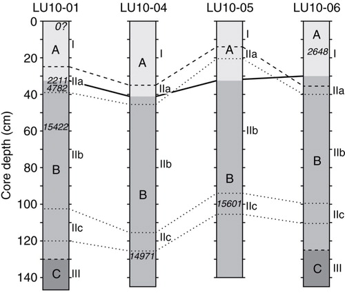
Fig. 8 Biostratigraphic correlations among the cores (solid lines). Assemblage Zones (A, B and C; shades of grey), lithological units (I, II and III; dashed lines) and subunits (IIa, IIb, and IIc; dotted lines) are marked. Ages (Ky B.P.) are also indicated.
Assemblage Zone C. This assemblage is found in Lithological Unit III. It is characterized by the presence of cassidulinids other than C. reniforme, but in contrast to Zone A there is a considerable proportion of Islandiella spp. (). Elphidium spp. and C. reniforme are common, but not as dominant as in Zone B. Planktic foraminifera are common, with N. pachyderma predominating (>90%, ).
Assemblage Zone B. This zone is ca. 100 cm thick and is found in Lithological Unit II. Total foraminiferal abundance per unit weight of dry sediment shows a peak around 70–80 cm depth in core LU10-01 (), within Subunit IIb (laminated package). The zone is marked by the presence of Elphidium spp. together with C. reniforme (). Elphidium is generally dominant and can reach almost 100%, but the top and/or bottom of the zone may also contain peaks of Nonionellina labradorica, Stainforthia and Cibicides. Cassidulinids (apart from C. reniforme, ) and planktic foraminifers () are absent or rare. A sparse planktic fauna dominated by T. quinqueloba is found in the 40–60 cm interval in core LU10-06 ().
Assemblage Zone A. This zone is found in Lithological Unit I, presumably representing the Holocene sediment cover. Total foraminiferal abundance per unit weight of dry sediment increases suddenly from Zone B to Zone A (). Zone A is dominated by Epistominella pusilla with subsidiary Cibicides spp., Cassidulina neoteretis and Melonis barleeanus, and abundant planktic foraminifers (). Elphidium spp. and C. reniforme are notably absent. The fauna is both abundant and species-rich, with minor taxa including Stainforthia spp., P. bulloides, Fissurina sp., Lagena spp. and Uvigerina sp. The planktic component is dominated by N. pachyderma, but with N. incompta, T. quinqueloba, G. uvula and G. bulloides also common (). Sponge spicules can be very abundant, especially in the upper part of the unit.
Discussion
Environment prior to the deglaciation
The oldest lithological unit encountered (Unit III, , m, n) is a diamicton and is interpreted as glacial till. This interpretation is supported by the lack of stratification and the quite homogeneous abundance of gravel particles across the cores (Licht et al. Citation1999). The scarcity of datable material did not allow us to obtain a radiocarbon age for the unit, but it must be older than the 15.6 Ky B.P. obtained near the base of the overlying Lithological Unit II (, ). The foraminiferal content (Zone C, , ) may be glacially reworked. Rare Bulimina marginata in Zone C are opaque and abraded. Hald et al. (Citation1990) reported B. marginata at 10–12 m core depth in core 7120/06-01 in the Ingøydjupet area, in a clearly disturbed sequence with reversed radiocarbon dates, and interpreted this occurrence as reworked. If in situ, the benthic foraminifera (Elphidium and Cassidulina reniforme) would likely indicate a glaciomarine setting (see below), while the planktic fauna could be interpreted as full marine but cold water, dominated by Neogloboquadrina pachyderma. This diamicton may be correlated with one described from the southern part of Ingøydjupet and interpreted as a subglacial till (Unit 6, Junttila et al. Citation2010). Similar diamictons have been reported elsewhere from the Barents Sea, and some of them were suggested to have undergone compression by glacial load (e.g., Unit IV, Ivanova et al. Citation2002). Unit III can be related to the Stage 1 of the Late Weichselian events in the south-western Barents Sea described by Winsborrow et al. (Citation2010). This period corresponds to the glacial maximum after 19 Ky B.P., with ice streams operating in Bjørnøyrenna and other troughs such as Ingøydjupet.
Early deglaciation
The beginning of the deglaciation is marked by the deposition of coarse material with abundant gravel particles (>2000 µm) in the 10-cm-thick layer at the bottom of Lithological Unit II (Subunit IIc, , i–l). This material is interpreted as IRD resulting from increased calving of icebergs from the marine ice-sheet margin (Aagaard-Sørensen et al. Citation2010), which was mainly triggered by sea-level rise (Winsborrow et al. Citation2010). Glacial unloading and rising seawater temperatures during the early deglaciation destabilized methane hydrate deposits, leading to free gas release through the seafloor and the formation of the pockmarks visible in the study area (; Chand et al. Citation2012; Nickel et al. Citation2012; Pau et al. Citation2014).
During the deposition of Subunit IIc, Nonionellina labradorica reached peak abundance in all cores investigated, marking the base of Assemblage Zone B (). This species often peaks within the later stages of the Late Weichselian deglaciation in the north-east Atlantic (Knudsen and Austin Citation1996). Another noteworthy foraminifer peaking at the base of Zone B is Stainforthia (). This is a highly opportunistic genus (e.g., Alve Citation2003), often dominating in areas of rapid environmental change. In the Arctic region, Stainforthia is typically abundant in areas with seasonal sea-ice cover or sea-ice margins (Seidenkrantz Citation2013).
The timing of the IRD event of Subunit IIc is constrained between 15.6 and 15.0 Ky B.P. (, , ). The age of 15.0 Ky B.P. is in line with the results published by Pau et al. (Citation2014), who correlate it with the base of Lithological Unit II. Part of the discrepancy with the age of 15.6 Ky B.P. may result from large uncertainty in the radiocarbon calibration curve at the beginning of the Bølling warming (Reimer et al. Citation2013) related to rapid and uneven sea-level rise resulting from meltwater pulses (e.g., Deschamps et al. Citation2012). Two deglacial IRD events were found in Ingøydjupet, of which the older one is estimated to have occurred at 15.1 Ky B.P. (Period I, Aagaard-Sørensen et al. Citation2010). This IRD event can possibly be correlated with our Subunit IIc. Junttila et al. (Citation2010) report a shift from diamicton to IRD abundance in Ingøydjupet (Units 5 and 4), dating it to 15.0 Ky B.P. Based on a peak in N. labradorica similar to that found in the present study, Chistyakova et al. (Citation2010) estimate the deglaciation to have commenced in Ingøydjupet between 14.2 and 13.8 Ky B.P. Age variations between different sites might reflect a difference in time for the position of the ice margin, but more ages are needed to evaluate this pattern. Winsborrow et al. (Citation2010) assign the age of ca. 16 Ky B.P. to the onset of glaciomarine conditions in the south-western Barents Sea (Stage 3) and ca. 15 Ky B.P. to the complete loss of the ice cover in the region (Stage 4).
The laminated package immediately above the IRD layer (Lithological Subunit IIb, , e–h) likely documents high sedimentation rates in a glaciomarine environment (e.g., Ó Cofaigh & Dowdeswell Citation2001 and references therein). The fauna is dominated by Elphidium spp., typical of ice-marginal settings, and C. reniforme, a cold-water indicator (). Furthermore, the absence of planktic foraminifera in the lower part of Zone B (, ) is consistent with a glaciomarine environment (see also the barren planktic zone PFZ-0 of Aagaard-Sørensen et al. Citation2010). The age of 15.4 Ky B.P. in the upper part of the laminated sediment (core LU10-01) is within the error range of the age from the preceding IRD event in adjacent cores (, , ), possibly in relation to high sedimentation rates. The lamination has a gradational basal contact with the IRD layer and is characterized by planar and parallel laminae, occurrence of iceberg dropstones and no bioturbation, probably due to the negative effect of high sedimentation rate on macrofauna (e–h). These features correspond to diagnostic criteria for the deposition of laminae by suspension-settling in an ice-proximal environment (Ó Cofaigh & Dowdeswell Citation2001). The thickness of the laminae of about 0.2 cm (e–h), however, is not high enough to imply a direct proximity to the ice edge (Ó Cofaigh & Dowdeswell Citation2001). The alternating sand and mud laminae may represent annual couplets reflecting seasonally variable meltwater discharge, in which case they can be classified as glaciomarine varves (Ó Cofaigh & Dowdeswell Citation2001). A similar interval of laminated sediments is reported from Ingøydjupet by Aagaard-Sørensen et al. (Citation2010) and Junttila et al. (Citation2010), where the timing of their deposition is related to the Older Dryas (ca. 14.6–14.5 Ky B.P.). In the central part of the Barents Sea, Ivanova et al. (Citation2002) also describe a laminated sequence overlying sediments with abundant IRD (Unit II and III, respectively). They relate the deposition of the laminae to glacier meltwater discharge, following an initial phase of ice-sheet disintegration.
The peak in the total number of foraminiferal specimens per unit weight of dry sediment found in Zone B of core LU10-01 () could be due to increased foraminiferal productivity along with a local ecological change. Since the laminae do not show a decrease in thickness, this peak is not explainable in terms of reduced sedimentation rate. Moreover, considering Zone B is barren of planktic foraminifera, we cannot relate it to the peak abundance of planktic species found in similar facies by Aagaard-Sørensen et al. (Citation2010) and Junttila et al. (Citation2010). Ivanova et al. (Citation2002) report no such peak from the central Barents Sea either.
In core LU10-06, there is an interval near the top of Lithological Unit II (40–55 cm core depth, ) with an initial, moderate influx of planktic foraminifera dominated by the subpolar species T. quinqueloba. This indicates a warmer surface water pulse terminating the glaciomarine environments. For a comparison, in the Fram Strait area T. quinqueloba predominates close to the sea-ice margin in water masses influenced by the Atlantic Water (Volkmann Citation2000). In contrast to a similar, but apparently younger (base Holocene) peak of T. quinqueloba found by Aagaard-Sørensen et al. (Citation2010) in Ingøydjupet, the accompanying benthic foraminiferal community (Elphidium spp. and C. reniforme) is still distinctly glaciomarine in core LU10-06. Moreover, the near-absence of C. neoteretis indicates no considerable Atlantic Water influence on the benthic fauna at this time. The 63-µm sieve size used in the present study may have enabled detection of this planktic faunal event, which studies based on a larger mesh size (e.g., Aagaard-Sørensen et al. Citation2010, 100 µm) would fail to detect.
Late deglaciation
The disconformity at the top of the laminated sediments (e) appears to be a result of bottom-current erosion. Readvance of grounded ice as an agent of erosion is unlikely, especially in the context of well-preserved pockmarks in the study area (). We hypothesize that the intensification of bottom currents was linked to a climatic deterioration and the associated sea-surface cooling and sea-ice formation, hence increased production of brines, possibly during the Older Dryas (ca. 14.6–14.5 Ky B.P.). Evidence for intense brine formation in a Svalbard fjord coinciding with the Older Dryas (Rasmussen & Thomsen Citation2014) supports this interpretation.
The coarse-grained material deposited on top of the disconformity is interpreted as IRD (Subunit IIa, , e, c). Although less prominent than in Subunit IIc, this IRD likely represents a second pulse of enhanced iceberg production from the decaying ice sheet and can be tentatively correlated with the Allerød interstadial (ca. 14–13 Ky B.P.). Both the erosion event and the deposition of Subunit IIa occurred subsequent to the onshore retreat of the ice margin (Winsborrow et al. Citation2010, Stage 4, ca. 15 Ky B.P.).
No dates are available for the interval contained between 15.0 and 4.8 Ky B.P. (), likely indicating a major hiatus at the bottom of the Holocene (c), probably due to erosion by bottom currents. No such hiatus is reported from Ingøydjupet (Aagaard-Sørensen et al. Citation2010; Chistyakova et al. Citation2010; Junttila et al. Citation2010); nonetheless, the authors provide micropaleontological evidence for high-energy bottom environments in the Early Holocene (Aagaard-Sørensen et al. Citation2010; Chistyakova et al. Citation2010). The difference in water depth between the present study area and Ingøydjupet corresponds to about 50 m, suggesting topography-controlled local variations in the hydrodynamic regime. Aagaard-Sørensen et al. (Citation2010) and Chistyakova et al. (Citation2010) link the increased bottom-current activity to a strengthening of the Atlantic current, consistent with a regional trend for the Barents Sea (Hald et al. Citation2007; Risebrobakken et al. Citation2010).
Near the boundary between Assemblage Zones A and B, the investigated cores exhibit intermittent absence of planktic foraminifera, together with a very low-abundance benthic fauna. This thin, barren interval could possibly reflect the Younger Dryas cold event dated in Ingøydjupet to 12.70–11.65 Ky B.P. by Aagaard-Sørensen et al. (Citation2010) and to 12.8–11.3 Ky B.P. by Chistyakova et al. (Citation2010).
Late Holocene
The Holocene sedimentary record recovered is characterized by deposition of marine mud with an abundant bioclastic component (Lithological Unit I, , a–d). The earliest date that can be provided for the Holocene material is 4.8 Ky B.P. (). This age, obtained on fragments of a thin-shelled bivalve from the top of the underlying Assemblage Zone B (), presumably represents the age for the bottom of Zone A as bivalves may move vertically up to a few tens of centimetres in their burrow. Mixed shell fragments recovered from the middle of Lithological Unit I/Assemblage Zone A are of late Holocene age (2.6 Ky B.P., , , , ).
The hiatus between Units II and I is marked by a relatively abrupt change in the taxonomic composition of the foraminiferal assemblage, accompanied by a significant increase in the species richness and abundance (Assemblage Zone A, CitationFigs. 5–Citation7). The latter is explainable in terms of reduced sedimentation rate in the Holocene, and probably also downcore dissolution of the carbonate tests. The abundance of planktic foraminifers (, ) indicates full marine conditions. The increased influence of Atlantic Water is illustrated by a common occurrence of Cassidulina neoteretis (Mackensen & Hald Citation1988). Furthermore, high abundance of Cibicides spp., with a peak dated to ca. 2.2 Ky B.P. in one of the cores (, ), suggests high bottom-current velocities. A similar faunal change, found elsewhere in the western Barents Sea, has been explained by the influence of Atlantic water masses and increased bottom currents (Ivanova et al. Citation2002; Aagaard-Sørensen et al. Citation2010; Chistyakova et al. Citation2010). The topmost 20–30 cm interval in some cores under this study is characterized by a reduction in C. neoteretis, with Epistominella pusilla becoming dominant, reaching 70% at the core top. A similar development in benthic foraminifers during the Holocene was noted in Ingøydjupet by Chistyakova et al. (Citation2010). The increase of E. pusilla reflects warm Atlantic Water, increasing bottom currents and unstable flux of organic matter to the seafloor (Rasmussen et al. Citation2007; Chistyakova et al. Citation2010).
Conclusions
Based on a lithological and foraminiferal investigation of sediment cores retrieved in the south-western Barents Sea, three lithofacies and associated foraminiferal assemblage zones were identified. This stratigraphy represents a transition from subglacial to glaciomarine and marine depositional environments. Based on the available 14C ages, deglaciation of the study area began prior to ca. 15.6–15.0 Ky B.P. An IRD layer was deposited during the initial disintegration of the ice sheet, possibly corresponding to the inception of the Bølling interstadial. Overlying laminated glaciomarine sediments were likely deposited in proximity to the retreating ice-sheet margin. A major depositional hiatus, loosely bracketed by the ages of 15.0 and 4.8 Ky B.P., separates deglacial and Holocene sediments. The hiatus presumably indicates high bottom-current activity, probably linked to a strengthening of the inflow of Atlantic Water into the Barents Sea with the onset of Holocene environments.
Supplementary Material
Download PDF (599.8 KB)Acknowledgements
Harald Brunstad and Lundin Petroleum Norway are warmly thanked for financial support and for providing the cores. For the excellent support during the expedition, a sincere gratitude goes to Arnfinn Karlsen, Helge Jubskås, Martin Syre Wiig, Kjetil Bergh Ånonsen and Jon Otto Buer from the Norwegian Defence Research Establishment, as well as to the officers and crew of RV H.U. Sverdrup II, Johnny Remøy (captain), Terje Haugen, Erling Olsen, Henning Bergsnes, John Johnsen, Bernt Nilsen and Liv Sørensen. Arnfinn Karlsen is thanked also for the logistical assistance. Haflidi Haflidason at the University of Bergen is gratefully acknowledged for the assistance with core logging. Knut Dalen at the Norwegian University of Life Sciences is thanked for assistance with CT scanning, and Mufak Naoroz at the University of Oslo for support with grain size analysis. The article benefited from comments and suggestions by Leonid Polyak and other reviewers.
Notes
To access the supplementary material for this article, please see the supplementary file under Article Tools, online.
References
- Aagaard-Sørensen S., Husum K., Hald M., Knies J. Paleoceanographic development in the SW Barents Sea during the Late Weichselian–Early Holocene transition. Quaternary Science Reviews. 2010; 29: 3442–3456.
- Alve E. A common opportunistic foraminiferal species as an indicator of rapidly changing conditions in a range of environments. Estuarine, Coastal and Shelf Science. 2003; 57: 501–514.
- Andreassen K., Laberg J.S., Vorren T.O. Seafloor geomorphology of the SW Barents Sea and its glaci-dynamic implications. Geomorphology. 2008; 97: 157–177.
- Bellec V., Wilson M., Bøe R., Rise L., Thorsnes T., Buhl-Mortensen L., Buhl-Mortensen P. Bottom currents interpreted from iceberg ploughmarks revealed by multibeam data at Tromsøflaket, Barents Sea. Marine Geology. 2008; 249: 257–270.
- Bigg G.R., Clark C.D., Greenwood S.L., Haflidason H., Hughes A.L.C., Levine R.C., Nygård A., Sejrup H.P. Sensitivity of the North Atlantic circulation to break-up of the marine sectors of the NW European ice sheets during the last glacial: a synthesis of modelling and palaeoceanography. Global and Planetary Change. 2012; 98/99: 153–165.
- Bjarnadóttir L.R., Rüther D.C., Winsborrow M.C.M., Andreassen K. Grounding-line dynamics during the last deglaciation of Kveithola, W Barents Sea, as revealed by seabed geomorphology and shallow seismic stratigraphy. Boreas. 2012; 42: 84–107.
- Boespflug X., Long B.F.N., Occhietti S. CAT-scan in marine stratigraphy: a quantitative approach. Marine Geology. 1995; 122: 281–301.
- Chand S., Thorsnes T., Rise L., Brunstad H., Stoddart D., Bøe R., Lågstad P., Svolsbru T. Multiple episodes of fluid flow in the SW Barents Sea (Loppa High) evidenced by gas flares, pockmarks and gas hydrate accumulation. Earth and Planetary Science Letters. 2012; 331/332: 305–314.
- Chistyakova N.O., Ivanova E.V., Risebrobakken B., Ovsepyan E.A., Ovsepyan Y.S. Reconstruction of the postglacial environments in the southwestern Barents Sea based on foraminiferal assemblages. Oceanology. 2010; 50: 573–581.
- Clark P.U., Dyke A.S., Shakun J.D., Carlson A.E., Clark J., Wohlfarth B., Mitrovica J.X., Hostetler S.W., McCabe A.M. The Last Glacial Maximum. Science. 2009; 325: 710–714.
- Deschamps P., Durand N., Bard E., Hamelin B., Camoin G., Thomas A.L., Henderson G.M., Okuno J., Yokoyama Y. Ice-sheet collapse and sea-level rise at the Bølling warming 14,600 years ago. Nature. 2012; 483: 559–564.
- Elverhøi A., Fjeldskaar W., Solheim A., Nyland-Berg M., Russwurm L. The Barents Sea Ice Sheet—a model of its growth and decay during the last ice maximum. Quaternary Science Reviews. 1993; 12: 863–873.
- Grosfeld K., Sandhäger H. The evolution of a coupled ice shelf–ocean system under different climate states. Global and Planetary Change. 2004; 42: 107–132.
- Hald M., Andersson C., Ebbesen H., Jansen E., Klitgaard-Kristensen D., Risebrobakken B., Salomonsen G.R., Sarnthein M., Sejrup H.P., Telford R.J. Variations in temperature and extent of Atlantic Water in the northern North Atlantic during the Holocene. Quaternary Science Reviews. 2007; 26: 3423–3440.
- Hald M., Danielsen T.K., Lorentzen S. Late Pleistocene–Holocene benthic foraminiferal distribution in the southwestern Barents Sea: paleoenvironmental implications. Boreas. 1989; 18: 367–388.
- Hald M., Sættem J., Nesse E. Middle and Late Weichselian stratigraphy in shallow drillings from the southwestern Barents Sea: foraminiferal, amino acid and radiocarbon evidence. Norwegian Journal of Geology. 1990; 70: 241–257.
- Hammer Ø., Harper D.A.T., Ryan P.D. PAST: paleontological statistics software package for education and data analysis. Palaeontologia Electronica. 2001; 4( 1 ): article no. 4.
- Heroy D.C., Anderson J.B. Radiocarbon constraints on Antarctic Peninsula Ice Sheet retreat following the Last Glacial Maximum (LGM). Quaternary Science Reviews. 2007; 26: 3286–3297.
- Hillenbrand C.-D., Melles M., Kuhn G., Larter R.D. Marine geological constraints for the grounding-line position of the Antarctic Ice Sheet on the southern Weddell Sea shelf at the Last Glacial Maximum. Quaternary Science Reviews. 2012; 32: 25–47.
- Hughes T. A simple holistic hypothesis for the self-destruction of ice sheets. Quaternary Science Reviews. 2011; 30: 1829–1845.
- Ingólfsson Ó., Landvik J.Y. The Svalbard–Barents Sea ice-sheet—historical, current and future perspectives. Quaternary Science Reviews. 2013; 64: 33–60.
- Ivanova E.V., Murdmaa I.O., Duplessy J.-C., Paterne M. Late Weichselian to Holocene paleoenvironments in the Barents Sea. Global and Planetary Change. 2002; 34: 209–218.
- Joughin I., Alley R.B. Stability of the West Antarctic ice sheet in a warming world. Nature Geoscience. 2011; 4: 506–513.
- Junttila J., Aagaard-Sørensen S., Husum K., Hald M. Late Glacial–Holocene clay minerals elucidating glacial history in the SW Barents Sea. Marine Geology. 2010; 276: 71–85.
- Knudsen K.L., Austin W.E.N. Andrews J.T. Late glacial foraminifera. Late Quaternary palaeoceanography of the North Atlantic Margin. 1996; London: The Geological Society. 7–10.
- Lambeck K. Limits on the areal extent of the Barents Sea ice sheet in Late Weichselian time. Global and Planetary Change. 1996; 12: 41–51.
- Landvik J.Y., Bondevik S., Elverhøi A., Fjeldskaar W., Mangerud J., Salvigsen O., Siegert M.J., Svendsen J.-I., Vorren T.O. The last glacial maximum of Svalbard and the Barents Sea area: ice sheet extent and configuration. Quaternary Science Reviews. 1998; 17: 43–75.
- Larrasoaña J.C., Roberts A.P., Musgrave R.J., Gràcia E., Piñero E., Vega M., Martínez-Ruiz F. Diagenetic formation of greigite and pyrrhotite in gas hydrate marine sedimentary systems. Earth and Planetary Science Letters. 2007; 261: 350–366.
- Licht K.J., Dunbar N.W., Andrews J.T., Jennings A.E. Distinguishing subglacial till and glacial marine diamictons in the western Ross Sea, Antarctica: implications for a last glacial maximum grounding line. Geological Society of America Bulletin. 1999; 111: 91–103.
- Mackensen A., Hald M. Cassidulina teretis Tappan and C. laevigata d'Orbigny: their modern and late Quaternary distribution in the northern seas. Journal of Foraminiferal Research. 1988; 18: 16–24.
- Mangerud J., Gulliksen S. Apparent radiocarbon ages of recent marine shells from Norway, Spitsbergen and Arctic Canada. Quaternary Research. 1975; 5: 263–273.
- Nick F.M., Vieli A., Howat I.M., Joughin I. Large-scale changes in Greenland outlet glacier dynamics triggered at the terminus. Nature Geoscience. 2009; 394: 110–114.
- Nickel J.C., di Primio R., Mangelsdorf K., Stoddart D., Kallmeyer J. Characterization of microbial activity in pockmark fields of the SW-Barents Sea. Marine Geology. 2012; 332–334: 152–162.
- Ó Cofaigh C., Dowdeswell J.A. Laminated sediments in glacimarine environments: diagnostic criteria for their interpretation. Quaternary Science Reviews. 2001; 20: 1411–1436.
- Olsen L. Mid and Late Weichselian, ice-sheet fluctuations northwest of the Svartisen glacier, Nordland, northern Norway. Geological Survey of Norway Bulletin. 2002; 440: 39–52.
- Ottesen D., Dowdeswell J.A., Rise L. Submarine landforms and the reconstruction of fast-flowing ice streams within a large Quaternary ice sheet: the 2500-km-long Norwegian–Svalbard margin (57°–80° N). Geological Society of America Bulletin. 2005; 117: 1033–1050.
- Ottesen D., Rise L., Rokoengen K., Sættem J. Martinsen O.J., Dreyer T. Glacial processes and large-scale morphology on the mid-Norwegian continental shelf. Sedimentary environments offshore Norway—Palaeozoic to recent. 2001; Amsterdam: Elsevier. 439–447.
- Ottesen D., Stokes C.R., Rise L., Olsen L. Ice-sheet dynamics and ice streaming along the coastal parts of northern Norway. Quaternary Science Reviews. 2008; 27: 922–940.
- Pau M., Hammer Ø., Chand S. Constraints on the dynamics of pockmarks in the SW Barents Sea: evidence from gravity coring and high-resolution, shallow seismic profiles. Marine Geology. 2014; 355: 330–345.
- Rasmussen T.L., Thomsen E. Brine formation in relation to climate changes and ice retreat during the last 15,000 years in Storfjorden, Svalbard, 76–78°N. Paleoceanography. 2014; 29: 911–929.
- Rasmussen T.L., Thomsen E., Slubowska M.A., Jessen S., Solheim A., Koc N. Paleoceanographic evolution of the SW Svalbard margin (76°N) since 20,000 14C yr BP. Quaternary Research. 2007; 67: 100–114.
- Rebesco M., Liu Y., Camerlenghi A., Winsborrow M., Laberg J.S., Caburlotto A., Diviacco P., Accettella D., Sauli C., Wardell N., Tomini I. Deglaciation of the western margin of the Barents Sea Ice Sheet—a swath bathymetric and sub-bottom seismic study from the Kveithola Trough. Marine Geology. 2011; 279: 141–147.
- Reimer P.J., Bard E., Bayliss A., Beck J.W., Blackwell P.G., Bronk Ramsey C., Buck C.E., Cheng H., Edwards R.L., Friedrich M., Grootes P.M., Guilderson T.P., Haflidason H., Hajdas I., Hatté C., Heaton T.J., Hoffmann D.L., Hogg A.G., Hughen K.A., Kaiser K.F., Kromer B., Manning S.W., Niu M., Reimer R.W., Richards D.A., Scott E.M., Southon J.R., Staff R.A., Turney C.S.M., van der Plicht J. Intcal13 and Marine13 radiocarbon age calibration curves, 0–50,000 years cal BP. Radiocarbon. 2013; 55: 1869–1887.
- Reimer P.J., Reimer R.W. A marine reservoir correction database and on-line interface. Radiocarbon. 2001; 43: 461–463.
- Risebrobakken B., Moros M., Ivanova E.V., Chistyakova N., Rosenberg R. Climate and oceanographic variability in the SW Barents Sea during the Holocene. The Holocene. 2010; 20: 609–621.
- Rüther D.C., Mattingsdal R., Andreassen K., Forwick M., Husum K. Seismic architecture and sedimentology of a major grounding zone system deposited by the Bjørnøyrenna Ice Stream during Late Weichselian deglaciation. Quaternary Science Reviews. 2011; 30: 2776–2792.
- Seidenkrantz M.-S. Benthic foraminifera as palaeo sea-ice indicators in the subarctic realm—examples from the Labrador Sea–Baffin Bay region. Quaternary Science Reviews. 2013; 79: 135–144.
- Sejrup H.P., Hjelstuen B.O., Dahlgren K.I.T., Haflidason H., Kuijpers A., Nygård A., Praeg D., Stoker M.S., Vorren T.O. Pleistocene glacial history of the NW European continental margin. Marine and Petroleum Geology. 2005; 22: 1111–1129.
- Smith J.A., Hillenbrand C.-D., Kuhn G., Larter R.D., Graham A.G.C., Ehrmann W., Moreton S.G., Forwick M. Deglacial history of the West Antarctic Ice Sheet in the western Amundsen Sea Embayment. Quaternary Science Reviews. 2011; 30: 488–505.
- Stuiver M., Reimer P.J.2014. Accessed on the internet at http://calib.qub.ac.uk/calib/ on 31 January 2014..
- Svendsen J.I., Alexanderson H., Astakhov V.I., Demidov I., Dowdeswell J.A., Funder S., Gataullin V., Henriksen M., Hjort C., Houmark-Nielsen M., Hubberten H.W., Ingólfsson Ó., Jakobsson M., Kjær K.H., Larsen E., Lokrantz H., Lunka J.P., Lysa A., Mangerud J., Matiouchkov A., Murray A., Möller P., Niessen F., Nikolskaya O., Polyak L., Saarnisto M., Siegert C., Siegert M.J., Spielhagen R.F., Stein R. Late Quaternary ice sheet history of northern Eurasia. Quaternary Science Reviews. 2004; 23: 1229–1271.
- Volkmann R. Planktic foraminifers in the outer Laptev Sea and the Fram Strait—modern distribution and ecology. Journal of Foraminiferal Research. 2000; 30: 157–176.
- Vorren T.O., Kristoffersen Y. Late Quaternary glaciation in the south-western Barents Sea. Boreas. 1986; 15: 51–59.
- Vorren T.O., Laberg J.S. Andrews J.T. Late glacial air temperature, oceanographic and ice sheet interactions in the southern Barents Sea region. Late Quaternary palaeoceanography of the North Atlantic Margin. 1996; London: The Geological Society. 303–321.
- Vorren T.O., Lebesbye E., Larsen K.B. Dowdeswell J.A., Scourse J.D. Geometry and genesis of the glacigenic sediments in the southern Barents Sea. Glacimarine environments: processes and sediments. 1990; London: The Geological Society. 269–288.
- Winsborrow M.C.M., Andreassen K., Corner G.D., Laberg J.S. Deglaciation of a marine-based ice sheet: Late Weichselian palaeo-ice dynamics and retreat in the southern Barents Sea reconstructed from onshore and offshore glacial geomorphology. Quaternary Science Reviews. 2010; 29: 424–442.