Estimating sea-ice volume flux out of the Laptev Sea using multiple satellite observations

Abstract

Sea-ice outflow from the Laptev Sea is of considerable importance in maintaining the Arctic Ocean sea-ice budget. In this study, a method exclusively using multiple satellite observations is used to calculate sea-ice volume flux across the eastern boundary (EB) and northern boundary (NB) of the Laptev Sea during the October–November and February–March or March–April periods (corresponding to the ICESat autumn and winter campaigns) between 2003 and 2008. Seasonally, the mean total ice volume flux (i.e., NB+EB) over the investigated autumn period (1.96 km³/day) is less than that over the winter period (2.57 km³/day). On the other hand, the large standard deviations of the total volume flux, 3.45 and 0.91 km³/day for the autumn and winter campaigns, indicate significant interannual fluctuations in the calculated quantities. A statistically significant (P>0.99) positive correlation, R=0.88 (or 0.81), is obtained between volume flux across the EB (or NB) and mean ice-drift speed over the boundary for the considered 11 ICESat campaigns. In addition, statistics show that a large fraction of the variability in volume flux across the NB over the 11 investigated campaigns, roughly 40%, is likely explained by ice thickness variability. On average, flux through the Laptev Sea amounts to approximately one-third of that across Fram Strait during the autumn and winter campaigns. These large contributions of sea ice from the Laptev Sea demonstrate its importance as an ice source, affecting the entire sea-ice mass balance in the Arctic Ocean.

• Mass balance
• remote sensing
• climate change.

To access the supplementary material for this article, please see the supplementary file under Article Tools, online.

Arctic sea ice is one of the most visible components corresponding to climate changes (Serreze et al. 2008; Screen & Simmonds 2010) and is undergoing significant changes over the past three decades (Rigor & Wallace 2004; Stroeve et al. 2012). The extent of Arctic Ocean sea-ice cover has been observed to be declining at a rate of 4% per decade over a 32-year period (1979–2010) (Comiso 2012). The retreat of perennial ice (ice that has survived at least one summer melt season) is dramatic (Nghiem et al. 2007; Comiso 2012), occurring at a rate of 12.2% per decade over the 1979–2010 period (Comiso 2012). Along with these rapid shrinkages in sea-ice extent in the Arctic Ocean, substantial decreases in sea-ice thickness are also observed (Maslanik et al. 2007; Giles et al. 2008; Kwok et al. 2009; Maslanik et al. 2011). In particular, Kwok & Rothrock (2009) reported an astonishing decrease of 1.59 m in thickness when their estimates derived from ICESat measurements (2003–08) are compared with historical records from submarine profiles (1958–1976).

The decline of ice extent and thickness together constitutes a major loss in the Arctic sea-ice volume. Kwok et al. (2009) estimated a net ice loss of 5400 km³ in ON and 3500 m³ in FM for the ICESat period (2003–08). Moreover, based on new data from the radar altimeter onboard CryoSat-2, Laxon et al. (2013) reported a continued decline in Arctic sea-ice volume between the ICESat and CryoSat-2 periods: by 4291 km³ (36%) in autumn and 1479 km³ (9%) in winter (Laxon et al. 2013).

Understanding the variability of sea-ice volume stored in the Arctic Ocean requires knowledge of volume transport at the major fluxgates (Smedsrud et al. 2011). The main transport of sea ice out of the Arctic Ocean takes place via Fram Strait (Vinje 2001; Kwok, Cunningham et al. 2004), and a substantial part of ice export through Fram Strait is assumed to have originated as far away as the Siberian shelf seas on the opposite side of the Arctic Basin (Dethleff et al. 1998). Among the Siberian shelf seas, the Laptev Sea serves as one of the most important headwaters for sea-ice production (Kwok 2000; Krumpen et al. 2011). About 20% of the ice outflow through Fram Strait is expected to have originated from the Laptev Sea (Rigor & Colony 1997), giving it a key role in the fate of the Arctic sea ice (Alexandrov et al. 2000).

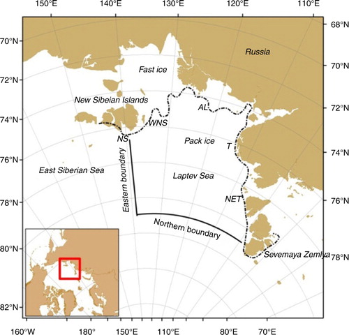
With shallow water depths between 15 and 200 m, the Laptev Sea is located between the coast of Siberia, Severnaya Zemlya and the New Siberian Islands and covered by sea ice from October to June (Fig. 1). It is occupied primarily by three ice regimes: the fast ice, pack ice and flaw polynyas. Because of persistent offshore winds, the pack ice is continuously pushed out of the Laptev Sea, entering into the Arctic Basin and/or the East Siberian Sea (Bareiss & Görgen 2005).

Fig. 1  Geographic location of the Laptev Sea, modified from Krumpen et al. (2013). The NB and EB used to calculate volume flux are marked as solid black lines. The fast ice edge is indicated as a dashed line. On average, five polynyas are formed between pack ice and fast ice edge, including the New Siberian polynya (NS), the western New Siberian polynya (WNS), the Anabar–Lena polynya (AL), the Taymyr polynya (T) and the Northern Taymyr polynya (NET).

Limited ice thickness measurements have confined most previous studies to area fluxes of ice exchanges between the Laptev Sea and neighbouring regions (Alexandrov et al. 2000; Krumpen et al. 2013). Compared to area flux, volume flux is a more insightful parameter to interpret the Arctic Ocean mass balance. In this study, we will present estimates of sea-ice volume flux out of the Laptev Sea by combining multiple satellite acquisitions, using a similar approach as described by Spreen et al. (2009). Our study could be considered as complementary to that carried out by Krumpen et al. (2013), who investigated a longer time series of area flux through the Laptev Sea.

Data

To calculate sea-ice volume flux, we explore multiple satellite-based retrievals, including sea-ice area, drift and thickness. A brief description on these data sets and processing technique is given as follows.

Sea-ice concentration

The sea-ice concentration information used here is available at the University of Bremen (www.iup.uni-bremen.de/seaice/amsredata/asi_daygrid_swath/l1a/n6250/). The product is derived from 89 GHz brightness temperatures measured by the AMSR-E, using the ASI algorithm developed at the University of Bremen (Spreen et al. 2008). The use of the 89 GHz channel data leads to sea-ice concentration with a grid size of 6.25 km. The ASI ice concentration algorithm uses an empirical model to retrieve the ice concentration between 0 and 100%. The atmospheric influence over the open ocean is mostly filtered using empirical models (see equations 13 and 14 in Spreen et al. [2008]). Error estimates show that the algorithm produces appropriate results at mid and high ice concentrations. In particular, the error should not exceed 10% for a concentration above 65% (Spreen et al. 2008). However, substantial deviations may occur in areas with low ice concentration depending on atmospheric conditions.

Sea-ice drift

Sea-ice drift can be derived from pairs of time-lagged satellite images based on a maximum cross-correlation technique (Ezraty et al. 2007a, b), which has been operationally provided by the Center for Satellite Exploitation and Research at IFREMER. Assessments conducted by Rozman et al. (2011) show that the IFREMER drift product acquired from AMSR-E 89 GHz pair images with a time lag of three days has the better performance compared with product derived from Advanced Synthetic Aperture Radar images or low-resolution AMSR-E 37 GHz observations provided by European Organization for the Exploitation of Meteorological Satellites Ocean and Sea Ice Satellite Application Facility.

In this study, we use a synergy product that is merged using separately retrieved drift from time-lagged (three-day) horizontally and vertically polarized AMSR-E observations at 89 GHz (ftp://ftp.ifremer.fr/ifremer/cersat/proudts/gridded/psi-drift/data). The product is available on a polar stereographic projection at a 31.25-km pixel resolution. The synthesizing process is also completed at IFREMER. Through the combination, the synergy is expected to have an improved data density compared with any single products (Ezraty et al. 2007a). A detailed description related to the original data processing and product assessment is given by Ezraty et al. (2007).

Sea-ice freeboard and thickness

Near basin-wide freeboard has been acquired from observations of the Geoscience Laser Altimeter System onboard ICESat (Kwok et al. 2007). The sensor uses a 1064-nm laser channel for surface altimetry with an expected accuracy of 15 cm. As the laser measures the top of snow on the ice, if snow is present, the freeboard denotes the combined value for sea ice and snow. Its measurements have a resolution of 60 m across and 170-m along the track. The satellite orbit has an inclination of 94° and hence leaves a 4° observational hole around the North Pole.

ICESat was in orbit for almost six years, from 2003 to 2009, but was operating up to three separated periods each year. Tracks of ICESat freeboard have been provided by the National Snow and Ice Data Center (www.nsidc.org/data/docs/daac/nsidc0393_arctic_seaice_freeboard/). Details regarding the original data-processing methods and the freeboard retrieval technique are described by Zwally et al. (2002). Only the autumn and winter ICESat observations between 2003 and 2008 are used in this study. The specific time range of the corresponding campaign and the designation of each campaign are summarized (Supplementary Fig. S1).

Typically, there is a separation of four to five months between the ICESat fall and winter campaigns (Kwok et al. 2009). The five fall campaigns cover a period roughly from mid-October to mid-November (ON), whereas the six winter campaigns span from late February to late March (FM), except for 07MA, which spans from mid-March to mid-April 2007. Each campaign generally involves a period of observations approximately 30 days in length, except for the 03ON campaign, which includes a time range of 55 days (Supplementary Fig. S1, Supplementary Table S1). For consistency, only the one-month freeboard data, with approximately the same time range as the other ICESat autumn campaigns, are used to obtain the gridded thickness for the 03ON campaign.

Assuming ice density, water density and snow depth, ice freeboard can be converted to ice thickness by applying the Archimedes principle (Kwok, Zwally et al. 2004). The density of sea ice varies depending on the age of the ice, which is related to the amount of brine and air inclusions (Gloersen et al. 1973). FY ice containing a substantial amount of brine water is expected to have a higher density. MY ice is assumed to be less dense than FY ice because of the extensive brine drainage in summer and the inclusion of a porous ice structure. Accounting for the two ice densities, the freeboard-to-thickness conversion technique compatible for satellite laser altimetric measurements is given by Spreen et al. (2009) and written as1

where I is the ice thickness, f _s is the ice freeboard height,c is the total ice concentration, c _m is the MY ice fraction,s is the snow depth on ice, and ρ _w , ρ _m , ρ _f and ρ _s denote the densities of sea water, MY ice, FY ice and snow, respectively. Detailed information regarding the selected values for these parameters and their uncertainties is summarized in Table 1 and is explained below.

Table 1 Selected values and their uncertainties of input variables used in converting ICESat freeboard to thickness for both periods. See the explanation in the text for how the values were obtained.

Variable	FM/MA	Uncertainty for FM/MA	ON	Uncertainty for ON	References
MY ice density (ρ m )	887 kg/m^3	20 kg/m^3	887 kg/m^3	20 kg/m^3	Eicken et al. 1995
FY ice density (ρ f )	910 kg/m^3	20 kg/m^3	910 kg/m^3	20 kg/m^3	Weeks & Lee 1958; Schwarz & Weeks 1977
Snow density (ρ s )	320 kg/m^3	15 kg/m^3	250 kg/m^3	20 kg/m^3	Kwok & Cunningham 2008
Sea water density (ρ w )	1023.9 kg/m^3	0.5 kg/m^3	1023.9 kg/m^3	0.5 kg/m^3	Laxon et al. 2003
Total ice concentration (c)	AMSR-E 89 GHz	0.05	AMSR-E 89 GHz	0.05	Spreen et al. 2008
MY concentration (c m )	QuikSCAT	0.10	QuikSCAT	0.10	Kwok 2004
Snow depth (s)	MY: W99, FY: AMSR-E	5.9 for FM, 6.2 for MA, 7.0	MY: W99, FY: W99/2	4.2, 7.0	Warren et al. 1999; Brucker & Marku 2013

Among the variables, snow depth on top of sea ice is the most undefined one and our knowledge about it is very limited. According to the field observations from the Soviet drift stations between 1954 and 1991, Warren et al. (1999; henceforth W99) established a climatology of monthly snow depth by fitting a two-dimensional quadratic function for each month of the year independently. The climatology represents snow depth on MY ice as the Arctic Ocean was dominated by MY ice during those decades. Recent analyses of field snow radar data showed that, while the W99 is still representative of snow on MY ice, snow depth on FY ice is overestimated by W99 (Kurtz & Farrell 2011). In this study, snow depth on MY ice provided by W99 is maintained while snow load for the FY ice derived from AMSR-E observations at 19 and 37 GHz is used (Comiso et al. 2003). The mean and uncertainty of snow depth for the FY ice on an order of 0.0±7.0 cm is given by Brucker & Markus (2013), who compared AMSR-E snow depth with Operation IceBridge airborne data. The±value refers to standard deviation. W99 also reported the interannual variability for the snow climatology at individual months (October: 4.0 cm, November: 4.3 cm, February: 5.5 cm, March: 6.2 cm, April: 6.1 cm). The uncertainties of snow depth on MY ice over the ON, FM and MA campaigns (4.2, 5.9 and 6.2 cm) are determined as the average uncertainty of the corresponding months.

For snow densities, we use those provided by Kwok & Cunningham (2008), 320 and 250 kg/m³ for the investigated winter and fall periods, respectively. The assumed uncertainty of σ _ρs =20 kg/m³ (or 15 kg/m³) for the autumn (or winter) campaign is the standard deviation of the W99 snow densities for September, October and November (or February, March and April). We use a density of 925 kg/m³ with an uncertainty of σ _ρf =20 kg/m³ for FY ice (Weeks & Lee 1958; Schwarz & Weeks 1977), 887 kg/m³ with an uncertainty of σ _ρm =20 kg/m³ for MY ice (Eicken et al. 1995; Laxon et al. 2003) and 1023.9 kg/m³ (σ _ρw =0.5 kg/m³) for sea water for both the studied seasons (Laxon et al. 2003).

The total ice concentration (c) is derived from AMSR-E 89 GHz measurements using the ASI algorithm. Daily average gridded QuikSCAT backscatter data at a pixel resolution of 12.5 km are processed at the Brigham Young University (ftp://ftp.scp.byu.edu/data/qscat/SigBrw) and used in this study to calculate the MY ice fraction according to the technique described by Kwok (2004), who established a relationship between the MY ice fraction from high-resolution RADARSAT/Relative Global Positioning System images and sigma₀ backscatter from QuikSCAT. The uncertainties of the total ice concentration (5%) and MY ice concentration (10%) are, respectively, acquired from Spreen et al. (2008) and Kwok (2004).

After the numerical substitution of these variables in Eqn. 1, ice thickness can be calculated for the autumn and winter campaigns using Eqns. 2 and 3, respectively2 3

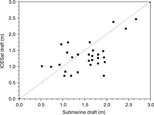
To examine the accuracy of our thickness estimates from ICESat freeboard, we have compared ice drafts (h _draft , i.e., ice thickness below the water surface) calculated from ICESat data (h _draft =I–f–s) to the ULS ice-draft measurements collected from four Beaufort Gyre Experiment Project moorings in the Beaufort Sea (www.whoi.edu/page.do?pid=66559). Following the method used by Kwok et al. (2009), we initially processed the point-wise mooring samples to produce twice-daily samples of the means and standard deviations of the ice drafts that are representative of those from 25-km tracks. This processing enables a statistically comparable spatial length between drafts obtained by ULS and ICESat. The time for the overhead ice pack to travelling a net distance of 25 km can be roughly calculated according to ice drift from the 89 GHz channels of AMSR-E (Ezraty et al. 2007). The mean ICESat ice drafts used in comparison are computed from segments within 25 km of the moorings and are closest in time with ULS observations (approximately within half a day). The ULS drafts are available over eight periods: 03ON, 04FM, 04ON, 05FM, 05ON, 06FM, 06ON and 07MA. Overall comparisons (Fig. 2) show that there is a mean difference of 0.21±0.45 m with the ICESat-based drafts being relatively underestimated, and a moderate correlation (R=0.56).

Fig. 2  Ice-draft comparison between submarine measurements and ICESat retrievals.

Methodology

Sea-ice volume flux out of the Laptev Sea

Ice volume flux is the product of ice concentration (c), drift velocity (D) and thickness (I). The volume flux through the NB and EB (Fig. 1), equivalent to borderlines used by Alexandrov et al. (2000) and Krumpen et al. (2013), is obtained in this study. The NB is positioned at the 81°N (100°–140°E) and the EB is located at the 140°E (77°–81°N) (Fig. 1). Sea-ice volume flux is given in the unit of km³/day. In the following, a positive (or negative) sign refers to an export out of (or import into) the Laptev Sea and the total volume flux corresponds to the sum of meridional volume flux across the NB and zonal volume flux through the EB.

The meridional (or zonal) volume flux V _m or (V _z ) for the NB (or EB) is the integral of volume flux estimate across each grid cell (i=1,…, n) located at the boundary and can be calculated with the following equation:4

where D _i is the meridional or zonal component of the sea-ice drift rate at the grid cell numbered as i, G is the length of the grid cell (25 km) and c _i is the ice concentration of the cell. Before used for volume flux computation, the daily ice concentration and ice-drift products are first interpolated to a 25-km grid and then averaged over a specific period (as that of ICESat campaign) to obtain c _i and D _i . I _i denotes the average thickness estimates of that “dropped” into a 25-km cell over a specific campaign.

Uncertainty estimation

The uncertainties of all input variables (assumed uncorrelated) propagated into the estimate of the meridional or zonal sea-ice volume flux can be calculated with the following equation:5

where σ _D,i , σ _I,i and σ _c,i are the uncertainties of ice drift, thickness and concentration, respectively, at the ith grid cell of the flux gate (summarized in Table 1).

Ice concentration in the Laptev Sea during the investigated periods are generally greater than 95%, where an uncertainty of 5% of ASI concentration obtained from Spreen et al. (2008) is used for the uncertainty estimate in Eqn. 5. The 5% threshold is also used by Spreen et al. (2008) in estimating the Fram Strait outflow uncertainty. For σ _D that represents the uncertainty of mean drift over an ICESat campaign period, we use (Spreen et al. 2008):6

where N is the number of valid sea-ice drift estimates for a grid cell over one ICESat campaign. The uncertainty of a single ice drift (σ _d ) is determined as 3.1 km/day by Ezraty et al. (2007) through a comparison between AMSR-E merged product and buoy drifts.

The uncertainty of the ice thickness (σ _I ), assuming a Gaussian uncertainty propagation from the input variables, can be given as7

where and . For detailed information about the selected values of all input variables and their uncertainties as used in Eqn. 7, refer to Table 1 and Sea-ice freeboard and thickness section.

Two sample maps of thickness uncertainty distribution are presented in Fig. 3. Other error maps look similar with the samples and are not shown here. Figure 4 shows that there is a larger uncertainty >0.5 m in the north of Greenland and Ellesmere Island coasts, where thicker MY ice prevails and uncertainties continuously reduce towards the peripheral areas, to an order of <0.2 m in the outskirt of the Arctic sea-ice regions.

Fig. 3  Spatial distribution maps of estimated uncertainty for sea-ice thickness for the (a) 07FM and (b) 07ON campaign.

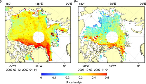
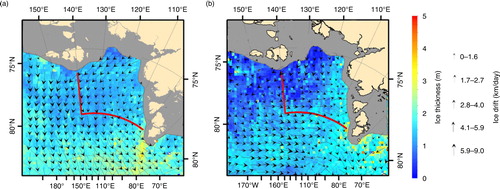
Fig. 4  Representative spatial distribution patterns of ice-drift vectors superimposed on the thickness estimates (blue to red) retrieved from the ICESat measurements. The maps represent the (a) winter and (b) autumn campaigns in 2003. The maps for the 2004–08 period are shown in Supplementary Fig. S2. The red lines represent the location of the two boundaries as indicated in Fig. 1.

The total uncertainty over the two fluxgates (σ _v ) can be achieved through8

where σ _vm and σ _vz , calculated according to Eqn. 5, are the uncertainties of the meridional and zonal volume flux estimates across the NB and EB, respectively.

Results

Spatial patterns of ice drift and ice thickness in the Laptev Sea

Figure 4 (also Supplementary Fig. S2) shows the spatial distributions of our thickness estimates in the Laptev Sea, superimposed with the IFREMER ice-drift vectors, over the autumn and winter campaigns during the period 2003–08. Depending on conditions of ice circulation, the direction of ice transport passing the two boundaries shows notable spatial variability. The campaigns mostly displayed a northward ice drift (i.e., offshore drift). However, the 06ON campaign (Supplementary Fig. S2f) showed an ice import pattern. For EB, either the easterly (export; Supplementary Fig. S2b, d, f) or westerly (import; Fig. 4b, Supplementary Fig. S2a, c, f) transport patterns of sea ice are observed. In particular, when a cyclonic drift was observed in Supplementary Fig. S2a, there was an enhanced westward ice inflow through EB. This pattern seems to be caused by a lower sea-level pressure after examining the corresponding data from the National Centers for Environmental Prediction/National Center for Atmospheric Research Reanalysis Project (Kalnay et al. 1996).

The spatial distribution of ice thickness is also presented in Fig. 4 and Supplementary Fig. S2. Seasonal differences in the ice thickness distribution pattern are notable. For the winter campaigns, the study area is mostly covered by FY ice with a moderate thickness, roughly 1.2–1.8 m. For the autumn campaigns, spatial patterns of ice thickness are complex. During the two earlier autumn periods—03ON (Fig. 4b) and 04ON (Supplementary Fig. S2b)—there is a marked thickness gradient from the southeastern (<1 m) to the northwestern (1.5–2.0 m) part of the Laptev Sea. Over the two latter periods (04/05ON; Supplementary Fig. S2d, f), the Laptev Sea is generally dominated by thinner FY ice. The ice thinning trend observed during the investigated ON periods is also quantitatively suggested in the time series of average thickness over the Laptev Sea between 2003 and 2008 (see Supplementary Fig. S3).

Temporal variability

Temporal variability of ice thickness over the Laptev Sea. The average sea-ice thickness over the Laptev Sea for the 11 ICESat campaigns is shown in Supplementary Fig. S3. The means varied both seasonally and interannually. Among these campaigns, the maximal thickness occurred in 05FM with a value of 1.7 m and the minimal took place in 06ON with a value of 0.62 m. On average, ice grows by 0.65 m over the growth period of roughly four to five months between the autumn and winter campaigns, from 0.86 to 1.51 m. Notable interannual variations can be concluded from the standard deviation of 0.22 m for both the autumn and the winter campaigns.

Considerable thickening was encountered in the 05ON/06FM and 06ON/07MA campaigns, with an autumn/winter increase of 0.9 and 1.01 m, respectively. The larger increase for the latter can be partially explained by the longer time span since the 07MA campaign, delayed approximately 20 days compared with 06FM. Other autumn/winter ice thickness experienced a relative moderate growth by an order of roughly half a metre.

Among the investigated periods, the 04ON/05FM seems like a watershed for the interannual variations of sea-ice thickness averaged over the Laptev Sea. For the autumn campaigns, the thickness dropped from 04ON till 06ON to as low as 0.6 m. For the winter campaigns, ice thickness in 05FM (1.70 m) increased strongly in comparison with that in 04FM (1.21 m). After 05FM, however, the winter thickness did not change markedly, with a mean value of 1.56 m and a small standard deviation of 0.15 m over the last four winter periods (i.e., 05/06FM, 07MA and 08FM).

Temporal variability of ice-drift rate over the Laptev Sea. Time series of the average of ice-drift rate for the zonal (D _z ) and meridional (D _m ) components and squared drift speed (D _v = sqrt[D _z ²+D _m ²]) over the Laptev Sea during the investigated period is shown in Fig. 5. During the 11 campaigns, the average speed of ice drifts (i.e., D _v ) over the Laptev Sea changes from 2.06 km/day (03ON) to 5.70 km/day (05ON). Seasonally, the average speed of ice drifts over the six winter campaigns (3.27 km/day) is close to that over the five autumn campaigns (3.77 km/day). Also, their standard deviation over the investigated autumn (1.18 km/day) approximates that of the winter periods (1.52 km/day), indicating large interannual variability in the calculated speed quantities for both the seasons.

Fig. 5  Ice-drift rate averaged over the Laptev Sea. D _m (in black) and D _z (in red) represent the mean meridional and zonal ice-drift rates, respectively. D _v (in blue) equals to denoting the drift magnitude. The vertical dashed lines are plotted for an easy discrimination drift rates of between autumn (blue) and winter (green) ICESat campaigns. A horizontal black dash line across zero is also given for a clear visual identification of the sign of a drift. A positive (or negative) meridional or zonal value defines a northward (or southward) transport or a westward (or eastward) transport. In other words, a positive (or negative) value indicates that ice is exported out of (or imported into) the Laptev Sea.

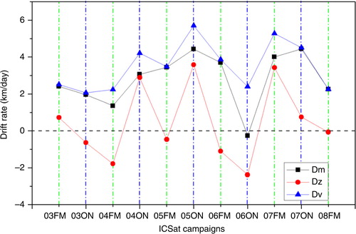
The meridional drift component across the NB in the Laptev Sea is primarily in a northerly direction, except in 06ON, when a weak southerly meridional transport emerged (Fig. 5, Supplementary Fig. S2f). Among the 11 campaigns, an overall maximum (or minimum) of meridional drift across the NB was observed in 05ON (or 06ON) with a rate of 5.7 km/day (or −0.27 km/day). In contrast, seasonal variability is relatively weak. There is a mean value of 2.86 (±1.01) km/day for the six winter campaigns and 2.73 (±1.97) km/day for the five autumn periods. However, the large standard deviations indicate a significant interannual variability in the meridional ice-drift component over the NB.

For the zonal component of ice drift across EB over the Laptev Sea, easterly (positive) and westerly (negative) ice transports were observed at times during the study period. There are six campaigns with negative zonal transport and five campaigns with positive zonal drift (Fig. 5). For the six negative campaigns, four cases took place in winter and two turned up in autumn. For the five positive campaigns, three cases emerged in autumn period and the remaining occurred in winter. Over the investigated period, the maximum (minimum) of absolute zonal drift rate over the EB occurred in 05ON (or 08FM) with a value of 3.58 km/day (or 0.10 km/day). Although averaged zonal drift rates over the EB are small for the six winter and five autumn campaigns (0.12 and 0.84 km/day, respectively). Although short and limited for data we used, the larger standard deviations in zonal drift over the EB (1.83 and 2.46 km/day for the winter and autumn campaigns, respectively), compared with those of the NB, confirm the fact that more remarkable interannual variability exists in the zonal ice-drift component compared with those of the meridional component (Krumpen et al. 2013).

Ice volume flux variability. Time series of seasonal and interannual variations in the volume flux of the Laptev Sea are shown in Fig. 6. The highest volume flux occurred in the 04ON period (roughly 7.8 km³/day), which is mainly due to the emergence of thicker ice with a relatively high transport rate around the NB boundary. Other relatively high ice outflow mainly took place during the winter periods (05/06/07), ranging from 3 to 4 km³/day. More interestingly, negative ice volume flux emerged for both the boundaries during the 06ON period, causing a strong ice import into the Laptev Sea, which is approximately −1 km³/day, the lowest net volume flux of the Laptev Sea among the 11 investigated periods.

Fig. 6  Time series of sea-ice volume flux estimates through the EB (v _z , orange) and NB (v _m , dark green) boundaries. Blue points denote the total flux (i.e., v _z +v _m ) with error bars showing the uncertainty calculated with Eqn. 8.

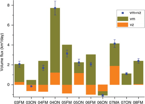
The means and standard deviations of the winter and autumn volume flux and their uncertainties over the period 2003–08 are summarized in Table 2. The noted large standard deviation suggested a larger fluctuations during autumn campaigns compared with the winter campaigns. The volume flux across the NB is generally larger in magnitude than that passing the EB. For EB, there is a mean autumn (or winter) transporting rate of 0.21±0.93 km³/day (or −0.06±1.09 km³/day). For the NB, the mean volume flux averaged over the autumn (or winter) periods is 1.75±2.72 (or 2.63±0.79) km³/day.

Table 2 Statistics of total volume flux and uncertainty as well as those of the zonal and meridional components across the EB and NB over the investigated period.

Period	EB	Uncertainty for EB	NB	Uncertainty for NB	Total	Uncertainty for the total flux
Winter	−0.06±1.08	0.22±0.05	2.63±0.79	0.60±0.15	2.57±0.91	0.58±0.10
Autumn	0.21±0.93	0.15±0.12	1.74±2.72	0.40±0.10	1.96±3.45	0.41±0.11

The mean increase between considered autumn and winter campaigns in the total flux of 0.61 km³/day is mainly attributable to increased ice thickness. There is an enhancement of ice export across the NB of 0.88 km³/day. Meanwhile, the volume flux at the EB shows a reversed transport between the autumn (0.21 km³/day) and winter (−0.06 km³/day) campaigns. The detailed seasonal behaviours of volume flux in the Laptev Sea over the considered ICESat periods are shown in Fig. 6. At the NB, increases are observed between the autumn and following winter volume fluxes, except for the 04ON/05FM campaigns, when a significant reduction of 2.49 km³/day (or 38%) occurred. For EB, there are complicated variations in volume flux since there are often events with direction reversals over the ICESat periods. For example, the 04ON/05FM (1.21/−0.87 km³/day) and 05ON/06FM (1.18/−0.99 km³/day) campaigns had a positive-to-negative transformation in flux orientation, whereas the direction change for the 06ON/07MA (−0.68/1.89 km³/day) and 07ON/08FM (−0.01/0.07 km³/day) campaigns was the opposite. Moreover, it is interesting to note an in-phase high ice exports across the two boundaries during the 07MA period, which would provide more extensive seasonal ice for the Arctic Basin in favour of the observed dramatic retreat of sea ice in the Arctic Ocean during the following melt seasons (Maslanik et al. 2007; Kwok & Cunningham 2008; Perovich et al. 2008).

The variability of volume flux is also remarkable over the investigated ICESat periods (Fig. 6). It varies between 1.68 km³/day (04FM) and 4.13 km³/day (07FM) over the winter record and between −1.08 km³/day (06ON) and 7.71 km³/day (04ON) over the autumn record. For the NB, volume flux alternates between −0.39 km³/day (06ON) and 6.49 km³/day (04ON) over the autumn record, and between 1.78 km³/day (03FM) and 4.01 km³/day (05FM) for the winter record. For EB, it changed from −0.068 km³/day (06ON) to 1.21 km³/day (04ON) over the autumn record and from −0.99 km³/day (06FM) to 1.89 km³/day (07FM) over the winter record.

The mean uncertainty of total volume flux in the winter campaigns (0.58±0.10 km³/day) is larger than that in autumn (0.41±0.11 km³/day). This seasonal contrast is also true for the volume flux estimates across the NB and EB (Table 2). Moreover, the volume flux across the NB is generally biased to a larger uncertainty compared with that across EB (Table 2).

Discussion

Comparisons to volume flux through Fram Strait

Fram Strait is the chief passage of the Arctic sea ice leaving the Arctic Ocean. In order to examine the role of ice import from the Laptev Sea in compensating ice loss due to export through the strait, we compare our volume flux estimates in the Laptev Sea to ice outflow through the strait.

Satellite-based estimates of sea-ice volume flux via the Fram Strait over the ICESat campaigns have been provided by Spreen et al. (2009), who explored a similar multi-sensor approach as used in this study. The transect in the Strait exploited by the authors is positioned at 80°N spanning a length of roughly 300 km between −20°E and 10°E.

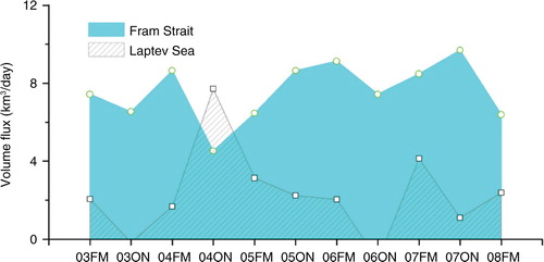
As seen in Fig. 7, a large fraction of Arctic sea-ice volume loss through the Fram Strait passage can be restored by ice injection from the Laptev Sea. The total volume export across the two Laptev Sea boundaries, on average, amounts to 35.9±48.6% of that through Fram Strait, with a mean percentage of 34.0±12.8 and 38.1±75.4% in the winter and autumn campaigns, respectively. In other words, more than one-third of volume loss due to Fram Strait exports is compensated by sea-ice input from the Laptev Sea during the investigated periods. These facts further demonstrate that ice import from the Laptev Sea is a vital role in maintaining Arctic mass balance. Particularly, the Arctic sea-ice volume received more ice from the Laptev Sea than loss due to outflow passing the Fram Strait during the 06ON period: 7.71 km³/day versus 4.53 km³/day (Fig. 7).

Fig. 7  Comparison between ice volume flux estimates through the Laptev Sea and Fram Strait. The Fram Strait outflow was obtained from Spreen et al. (2009).

Linkage between volume flux estimates and input variables

To examine the contribution of input variables to the sea-ice volume flux variability, the correlation is computed between volume flux estimates across the EB and NB and each input variable (ice concentration, drift rate and thickness) over the 11 ICESat campaigns. Results for the EB and NB are shown in Fig. 8 and Supplementary Fig. S4. The values for input variables shown in the figures correspond to the averages over the boundary.

Fig. 8  Time series of volume flux estimates at the NB along with a time series of values of parameters used to obtain the volume flux estimates. This figure represents the variability of sea-ice concentration (c), ice thickness (T), ice-drift rate (D) and ice volume flux (V) over the NB boundary.

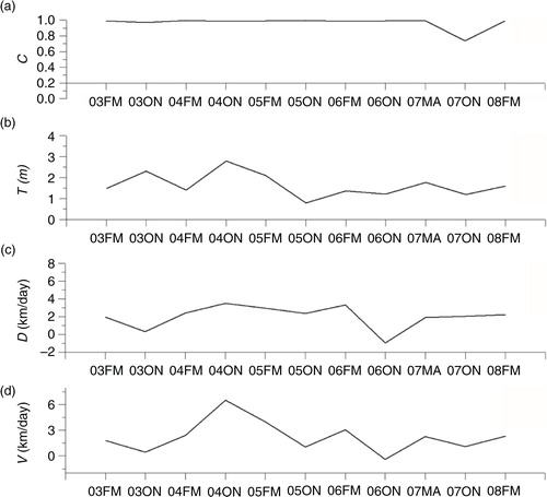
For the EB boundary, the ice volume flux time series showed a similar behaviour as that of ice-drift speed with a high correlation of 0.88 (significant at 99% level) (Supplementary Fig. S4c, d). By comparison, the thickness provided a negligible contribution to the volume flux variability of EB (R=0.15). Nevertheless, in the latter part of time series, from 06ON to 08FM, ice thickness variations remarkably affected the variability of volume flux (Supplementary Fig. S4b, d). Ice concentrations over EB did not show a notable variability throughout the study period and thus contributed the least to the behaviour of volume flux at the fluxgate (Supplementary Fig. S4a).

For the NB, the correlation between the volume flux estimates and mean drift speed (or ice thickness) is determined as 0.81 (or 0.65) at a significance level of 99% (or 95%). Therefore, for the NB the variability of volume flux is primarily controlled by the drift speed variability and secondly the ice thickness variability (Fig. 8b, c, d). For an inspection of the 11 estimates, ice thickness variations remarkably impacted the volume flux variability of the NB in the 04/05ON, 07ON and 08FM periods (Fig. 8b, d), while in the remaining periods the ice-drift speed variations exerted more influences on the changes of volume flux of the gate (Fig. 8c, d). In addition, small changes were observed in the ice concentration time series at the NB during the entire study period, except for the 07ON period, when a low ice concentration seemed to have imposed a great effect on producing a low volume flux estimate at the fluxgate in that period (Fig. 8a, d).

Conclusions

In this study, satellite-based retrievals of sea-ice concentration, drift rate and thickness are combined to calculate autumn and winter sea-ice volume flux through the two boundaries in the Laptev Sea between 2003 and 2008. Making use of the uniquely large spatio-temporal coverage of satellite observations, we are able to capture for the first time the seasonal and interannual behaviour of volume flux out of the Laptev Sea. Over the investigated 11 periods, we found that more than one-third of sea-ice volume outflow of the Arctic Ocean through the Fram Strait can be compensated by ice inflow from the Laptev Sea. This fact again points to that the Laptev Sea serves as one of the most important source regions providing sea ice to the Arctic Ocean, which is vital in affecting mass balance of the sea ice.

Since the 1980s, sea-ice outflow has been expected to be enhanced since a clear increase in the sea-ice drift speed has been found in the Laptev Sea (Spreen et al. 2011). On the other hand, there is a trend of general thinning sea-ice cover in the Arctic (Kwok & Rothrock 2009), which is partly attributable to a faster ice-drift speed. Thinner ice will lessen the volume of the outflow. A longer satellite record is needed as a basis for accurately determining the extent to which the interplay of increasing ice speed and decreasing ice thickness contributes to the volume flux variability in the Laptev Sea. Fortunately, the newly launched spaceborne instrument Cyrosat-2 provides us a good opportunity to extend the time series of our ice volume flux estimates, which is a part of our upcoming study.

Acknowledgements

We thank the organizations that provided the data used in this study: the Woods Hole Oceanographic Institution (Beaufort Gyre Experiment Project ice draft), the National Snow and Ice Data Center (ice concentration fields and ICESat freeboard measurements), IFREMER (sea-ice drift fields) and Brigham Young University (QuikSCAT backscatter data). This work is supported by the National Natural Science Foundation of China (no. 41406215), the Postdoctoral Science Foundation of China (no. 2014M561971) and the Open Fund for the Key Laboratory of Marine Geology and Environment, Institute of Oceanology, Chinese Academy of Sciences under contract no. MGE2013KG07, and performed at the Key Laboratory of Marine Geology and Environment.

Notes

To access the supplementary material for this article, please see the supplementary file under Article Tools, online.

References

- Alexandrov V.Y., Martin T., Kolatschek J., Eicken H., Kreyscher M., Makshtas A.P. Sea ice circulation in the Laptev Sea and ice export to the Arctic Ocean: results from satellite remote sensing and numerical modeling. Journal of Geophysical Research. 2000; 105: 17143–17159.
- Bareiss J., Görgen K. Spatial and temporal variability of sea ice in the Laptev Sea: analyses and review of satellite passive-microwave data and model results, 1979 to 2002. Global Planetary Change. 2005; 48: 28–54.
- Brucker L., Markus T. Arctic-scale assessment of satellite passive microwave-derived snow depth on sea ice using Operation IceBridge airborne data. Journal of Geophysical Research—Oceans. 2013; 118: 2892–2905.
- Comiso J.C. Large decadal decline of the Arctic multiyear ice cover. Journal of Climate. 2012; 25: 1176–1193.
- Comiso J.C., Cavalieri D.J., Markus T. Sea ice concentration, ice temperature, and snow depth using AMSR-E data. IEEE Transactions on Geoscience and Remote Sensing. 2003; 41: 243–252.
- Dethleff D., Loewe P., Kleine E. The Laptev Sea flaw lead—detailed investigation on ice formation and export during 1991/1992 winter season. Cold Regions Science and Technology. 1998; 27: 225–243.
- Eicken H., Lensu M., Leppäranta M., Tucker W.B., Salmela A.J.G.O. Thickness, structure, and properties of level summer multiyear ice in the Eurasian sector of the Arctic Ocean. Journal of Geophysical Research—Oceans. 1995; 100: 22697–22710.
- Ezraty R., Ardhuin F., Croizé-Fillon D. Sea ice drift in the central Arctic using the 89 GHz brightness temperatures of the Advanced Microwave Scanning Radiometer. User's manual. 2007; Version 2. Brest: French Research Institute for Exploitation of the Sea.
- Ezraty R., Girard-Ardhuin F., Piollé J. Sea ice drift in the central Arctic combining QuikSCAT and SSM/I sea ice drift data. User's manual. 2007a; Version 2. Brest: French Research Institute for Exploitation of the Sea.
- Ezraty R., Girard-Ardhuin F., Piollé J. Sea ice drift in the central Arctic estimated from SeaWinds/QuikSCAT backscatter maps. User's manual. 2007b; Version 2.2. Brest: French Research Institute for Exploitation of the Sea.
- Giles K.A., Laxon S.W., Ridout A.L. Circumpolar thinning of Arctic sea ice following the 2007 record ice extent minimum. Geophysical Research Letters. 2008; 35: L22502,. doi: http://dx.doi.org/10.1029/2008GL035710.
- Gloersen P., Nordberg W., Schmugge T., Wilheit T., Campbell W. Microwave signatures of first-year and multiyear sea ice. Journal of Geophysical Research. 1973; 78: 3564–3572.
- Kalnay E., Kanamitsu M., Kistler R., Collins W., Deaven D., Gandin L., Iredell M., Saha S., White G., Woollen J., Zhu Y., Chelliah M., Ebisuzaki W., Higgins W., Janowiak J., Mo K.C., Ropelewski C., Wang J., Leetmaa A., Reynolds R., Jenne R., Joseph D. The NCEP/NCAR 40-year reanalysis project. Bulletin of the American Meteorological Society. 1996; 77: 437–471.
- Krumpen T., Hölemann J.A., Willmes S., Maqueda M., Busche T., Dmitrenko I.A., Gerdes R., Haas C., Heinemann G., Hendricks S. Sea ice production and water mass modification in the eastern Laptev Sea. Journal of Geophysical Research—Oceans. 2011; 116: C05014,. doi: http://dx.doi.org/10.1029/2010JC006545.
- Krumpen T., Janout M., Hodges K., Gerdes R., Girard-Ardhuin F., Hölemann J., Willmes S. Variability and trends in Laptev Sea ice outflow between 1992–2011. The Cryosphere. 2013; 7: 1–15.
- Kurtz N.T., Farrell S.L. Large-scale surveys of snow depth on Arctic sea ice from Operation IceBridge. Geophysical Research Letters. 2011; 38: L20505,. doi: http://dx.doi.org/10.1029/2011GL049216.
- Kwok R. Recent changes in Arctic Ocean sea ice motion associated with the North Atlantic Oscillation. Geophysical Research Letters. 2000; 27: 775–778.
- Kwok R. Annual cycles of multiyear sea ice coverage of the Arctic Ocean: 1999–2003. Journal of Geophysical Research—Oceans. 2004; 109: C11004,. doi: http://dx.doi.org/10.1029/2003JC002238.
- Kwok R., Cunningham G.F. ICESat over Arctic sea ice: estimation of snow depth and ice thickness. Journal of Geophysical Research—Oceans. 2008; 113,(C08010): doi: http://dx.doi.org/10.1029/2008JC004753.
- Kwok R., Cunningham G.F., Pang S.S. Fram Strait sea ice outflow. Journal of Geophysical Research—Oceans. 2004; 109: C01009,. doi: http://dx.doi.org/10.1029/2003JC001785.
- Kwok R., Cunningham G.F., Wensnahan M., Rigor I., Zwally H.J., Yi D. Thinning and volume loss of the Arctic Ocean sea ice cover: 2003–2008. Journal of Geophysical Research—Oceans. 2009; 114: C07005,. doi: http://dx.doi.org/10.1029/2009JC005312.
- Kwok R., Cunningham G.F., Zwally H.J., Yi D. Ice, Cloud, and Land Elevation Satellite (ICESat) over Arctic sea ice: retrieval of freeboard. Journal of Geophysical Research—Oceans. 2007; 112: C12013,. doi: http://dx.doi.org/10.1029/2006JC003978.
- Kwok R., Rothrock D.A. Decline in Arctic sea ice thickness from submarine and ICESat records: 1958–2008. Geophysical Research Letters. 2009; 36: L15501,. doi: http://dx.doi.org/10.1029/2009GL039035.
- Kwok R., Zwally H.J., Yi D. ICESat observations of Arctic sea ice: a first look. Geophysical Research Letters. 2004; 31: L16401,. doi: http://dx.doi.org/10.1029/2004GL020309.
- Laxon S., Peacock N., Smith D. High interannual variability of sea ice thickness in the Arctic region. Nature. 2003; 425: 947–950.
- Laxon S.W., Giles K.A., Ridout A.L., Wingham D.J., Willatt R., Cullen R., Kwok R., Schweiger A., Zhang J., Haas C., Hendricks S., Krishfield R., Kurtz N., Farrell S., Davidson M. CryoSat-2 estimates of Arctic sea ice thickness and volume. Geophysical Research Letters. 2013; 40: 732–737.
- Maslanik J., Stroeve J., Fowler C., Emery W. Distribution and trends in Arctic sea ice age through spring 2011. Geophysical Research Letters. 2011; 38: L13502,. doi: http://dx.doi.org/10.1029/2011GL047735.
- Maslanik J.A., Fowler C., Stroeve J., Drobot S., Zwally J., Yi D., Emery W. A younger, thinner Arctic ice cover: increased potential for rapid, extensive sea ice loss. Geophysical Research Letters. 2007; 34: L24501,. doi: http://dx.doi.org/10.1029/2007GL032043.
- Nghiem S., Rigor I., Perovich D., Clemente-Colón P., Weatherly J., Neumann G. Rapid reduction of Arctic perennial sea ice. Geophysical Research Letters. 2007; 34: L19504,. doi: http://dx.doi.org/10.1029/2007GL031138.
- Perovich D.K., Richter-Menge J.A., Jones K.F., Light B. Sunlight, water, and ice: extreme Arctic sea ice melt during the summer of 2007. Geophysical Research Letters. 2008; 35: L11501,. doi: http://dx.doi.org/10.1029/2008GL034007.
- Rigor I., Colony R. Sea-ice production and transport of pollutants in the Laptev Sea, 1979–1993. Science of the Total Environment. 1997; 202: 89–110.
- Rigor I.G., Wallace J.M. Variations in the age of Arctic sea-ice and summer sea-ice extent. Geophysical Research Letters. 2004; 31: L09401,. doi: http://dx.doi.org/10.1029/2004GL019492.
- Rozman P., Hoelemann J., Krumpen T., Gerdes R., Koeberle C., Lavergne T., Adams S. Validating satellite derived and modelled sea-ice drift in the Laptev Sea with in situ measurements from the winter of 2007/08. Polar Research. 2011; 30(7218): doi: http://dx.doi.org/10.3402/polar.v30i0.7218.
- Schwarz J., Weeks W.F. Engineering properties of sea ice. Journal of Glaciology. 1977; 19: 499–531.
- Screen J.A., Simmonds I. The central role of diminishing sea ice in recent Arctic temperature amplification. Nature. 2010; 464: 1334–1337.
- Serreze M., Barrett A., Stroeve J., Kindig D., Holland M. The emergence of surface-based Arctic amplification. The Cryosphere Discussions. 2008; 2: 601–622.
- Smedsrud L., Sirevaag A., Kloster K., Sorteberg A., Sandven S. Recent wind driven high sea ice area export in the Fram Strait contributes to Arctic sea ice decline. The Cryosphere. 2011; 5: 821–829.
- Spreen G., Kaleschke L., Heygster G. Sea ice remote sensing using AMSR-E 89-GHz channels. Journal of Geophysical Research—Oceans. 2008; 113: C02S03,. doi: http://dx.doi.org/10.1029/2005JC003384.
- Spreen G., Kern S., Stammer D., Hansen E. Fram Strait sea ice volume export estimated between 2003 and 2008 from satellite data. Geophysical Research Letters. 2009; 36: L19502,. doi: http://dx.doi.org/10.1029/2009GL039591.
- Spreen G., Kwok R., Menemenlis D. Trends in Arctic sea ice drift and role of wind forcing: 1992–2009. Geophysical Research Letters. 2011; 38: L19501, doi: http://dx.doi.org/10.1029/2011GL048970.
- Stroeve J.C., Serreze M.C., Holland M.M., Kay J.E., Malanik J., Barrett A.P. The Arctic's rapidly shrinking sea ice cover: a research synthesis. Climatic Change. 2012; 110: 1005–1027.
- Vinje T. Fram Strait ice fluxes and atmospheric circulation: 1950–2000. Journal of Climate. 2001; 14: 3508–3517.
- Warren S.G., Rigor I.G., Untersteiner N., Radionov V.F., Bryazgin N.N., Aleksandrov Y.I., Colony R. Snow depth on Arctic sea ice. Journal of Climate. 1999; 12: 1814–1829.
- Weeks W.F., Lee O.S. Observations on the physical properties of sea-ice at Hopedale, Labrador. Arctic. 1958; 11: 134–155.
- Zwally H., Schutz B., Abdalati W., Abshire J., Bentley C., Brenner A., Bufton J., Dezio J., Hancock D., Harding D. ICESat's laser measurements of polar ice, atmosphere, ocean, and land. Journal of Geodynamics. 2002; 34: 405–445.