Lagrangian analysis of sea-ice dynamics in the Arctic Ocean

Abstract

In this study, we present Lagrangian diagnostics to quantify changes in the dynamical characteristics of the Arctic sea-ice cover from 2006 to 2014. Examined in particular is the evolution in finite-time Lyapunov exponents (FTLEs), which monitor the rate at which neighbouring particle trajectories diverge, and stretching rates throughout the Arctic. In this analysis, we compute FTLEs for the Arctic ice-drift field using the 62.5 km daily sea-ice motion vector data from the European Organisation for the Exploitation of Meteorological Satellites Ocean and Sea Ice Satellite Application Facility. Results from the FTLE analysis highlight the existence of three distinct dynamical regions with strong stretching, captured by FTLE maxima or ridges. It is further shown that FTLE ridges are dominated by shear, with contributions from divergence in the Beaufort Sea. Localization of FTLE features following the 2012 record minimum in summertime sea-ice extent illustrates the emergence of an Arctic characterized by increased mixing. Results also demonstrate higher FTLEs in years when lower multi-year ice extent is observed.

• sea-ice dynamics
• FTLE
• Arctic Ocean
• Lagrangian diagnostics
• LAD

Recent studies have illustrated an increase in sea-ice drift speeds and deformation rates in the Arctic, attributed both to a poleward migration in cyclonic activity (Hakkinen et al. 2008; Kwok et al. 2013) and a weaker ice cover in recent decades, particularly following 2000 (Rampal et al. 2009; Spreen et al. 2011; Kwok et al. 2013). In an assessment of changes in BG circulation from 2003 to 2011, McPhee (2013) demonstrated the emergence of stronger currents at the periphery of the BG and southward shift in the BG centre. Strengthening of the TDS has also been observed from 1982 to 2009 and is attributed to reduced MYI coverage (Kwok et al. 2013), captured by increasing (decreasing) trends in seasonal (multi-year) ice over the last several decades (Maslanik et al. 2011; Comiso & Hall 2014).

Whereas Eulerian diagnostics depict behaviour associated with individual time slices, Lagrangian diagnostics provide an assessment of evolution in fluid flow and its underlying patterns (Haller & Yuan 2000). A Lagrangian interpretation of sea-ice dynamics in the Arctic enables identification of dynamical features associated with transport and mixing. This therefore provides a tool with which to quantify characteristic large-scale (on the order of several hundreds of kilometres) features in addition to the Eulerian characterizations such as the BG in the Canada Basin, the TDS over the central Arctic, and changes in their relative contributions to sea-ice drift in the Arctic within a rapidly changing (in terms of sea-ice extent, duration, thickness) ice cover.

Early Lagrangian studies of sea-ice dynamics examined trajectories of drifting buoys to investigate sea-ice dispersion in the context of organized and random motion using concepts from turbulence (Thorndike 1986a, b). Recent Lagrangian analyses have also used buoy trajectories to quantify sea-ice drift and deformation (Rampal et al. 2008; Rampal et al. 2009; Hutchings et al. 2011; Weiss 2013). Spatial and temporal scaling laws illustrated coupling in space and time in sea-ice deformation processes (Rampal et al. 2008). Increased drift and deformation rates from 1979 to 2009 were found in the central Arctic and have been attributed to sea-ice kinematics and accompanying reduction in ice cover strength (Rampal et al. 2009). Hutchings et al. (2011) demonstrated coherence in deformation over length scales exceeding 100 km on daily to weekly timescales. Hutchings & Rigor (2012) further demonstrated a transition to a younger, thinner ice cover in the Beaufort Sea region associated with a change in ice-drift regimes in the western Arctic and Beaufort Sea since 1998.

Abbreviations in this article

AMSR-E: Advanced Microwave Scanning Radiometer–Earth Observing System

ASCAT: Advanced Scatterometer

BG: Beaufort Gyre

EUMETSTAT: European Organisation for the Exploitation of Meteorological Satellites

FTLE: finite-time Lyapunov exponent

LAD: Lagrangian averaged divergence

MYI: multi-year ice

OSI SAF: Ocean and Sea Ice Satellite Application Facility

PDFs: probability distribution functions

SSM/I: Special Sensor Microwave Imager

SSMIS: Special Sensor Microwave Imager/Sounder

TDS: Transpolar Drift Stream

Relevant to the present analysis is a Lagrangian interpretation of sea-ice drift and more importantly sea-ice deformation of a gridded and satellite-derived ice-drift product. Recent Lagrangian studies used satellite-based ice-drift data to explore the age of ice (Fowler et al. 2003; Rigor & Wallace 2004; Maslanik et al. 2011; Stroeve et al. 2011), demonstrating significant loss in MYI, shorter recirculation times within the BG and accompanying reductions in summertime sea-ice extent (Rigor & Wallace 2004; Stroeve et al. 2011). A climatological assessment by Maslanik et al. (2011) examined ice age distributions for the March 1980–2011 time frame and identified a regional tipping point in the Canada Basin associated with disproportionate loss of MYI in this region.

In the present analysis, we focus on changes in the flow dynamics and FTLEs in particular. FTLEs monitor the rate at which neighbouring trajectories diverge most over a finite time interval (Lichtenberg & Lieberman 1992). Ridges (maxima) and trenches (minima) in FTLE fields provide a signature of structure in the underlying flow, known as Lagrangian coherent structures, or skeletons of fluid flows, that characterize repelling, attracting and shearing persistent features in flow dynamics (Haller & Yuan 2000; Haller 2002; Peacock & Haller 2013).

In contrast to the aforementioned Lagrangian sea-ice deformation studies that analysed small deformations over short timescales and limited spatial scales, the FTLE approach coupled with satellite-based velocity field possesses an inherent ability to capture large deformations, namely long-term persistent features of sea-ice deformation. Furthermore, it was noted by Rampal et al. (2009) that the deformation rate proxy used in their study did not allow for distinction between divergence/convergence and shear. By contrast, the Lagrangian averaged divergence diagnostic used in the present analysis and described further below enables identification of divergence- and shear-dominated FTLE ridges, and hence distinct dynamical regimes over the investigated time frame.

In this study, we present new Lagrangian diagnostics in the interpretation of sea-ice dynamics that provide a characterization of dispersion in sea ice and of the spatiotemporal evolution in sea-ice drift and deformation. Specifically, we present FTLE fields generated during winter and analyse spatiotemporal features characteristic of changes in sea-ice dynamics and dispersion. Examined in particular are: (i) FTLE fields as a characterization of large-scale sea-ice dynamical regimes in the Arctic; (ii) spatiotemporal evolution in FTLE fields in the Arctic from 2006 to 2014 and relative contributions of shear, divergence and normal repulsion to FTLE ridges. The overall objective is to provide an alternative characterization of sea-ice dispersion that also distinguishes between shear- and divergence-dominated FTLE ridges or regions of maximal stretching.

Methods

Lagrangian techniques provide important information about the behaviour of the system based on analysis of particles’ trajectories, which can be calculated based on a sequence of discrete velocity fields over a given time interval (or given as a sequence of buoy positions). It should be noted that all calculations in this paper are based on forward time trajectories over the November to April time frame for each year. In this section, we introduce the notation, techniques and boundary conditions that were used for the analysis.

Particle tracking

First we consider a two-dimensional, unsteady velocity field v ( x, t), where time t is defined on a finite interval [t ₀, t ₁]. In this velocity field, all trajectories satisfy the following ordinary differential equation:1

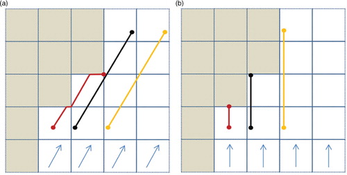
Particles are tracked by solving the equation of motion (Eqn. 1) with a variable step fourth- and fifth-order Runge–Kutta (also known as Dormand–Prince) scheme using bi-linear spatial interpolation, and initial conditions x ₀= x (t ₀) set up on an equally spaced grid. The non-trivial part of the algorithm was to find the appropriate boundary conditions. Since no-slip conditions generate artificial attractors at the boundaries, slip conditions were initially applied at lands and islands, and the “let them go” condition, whereby particles that reach the boundary are discarded, was applied for the melting region. It was, however, also found that slip conditions may create artificial trajectories due to interference with the boundaries (corner effect, boundary trapping), which cause artificial stretching, as shown in Fig. 1. Furthermore, the resolution of the data set does not allow us to investigate the deformation in the coastal region, especially the interaction with the passages of the Canadian Arctic Archipelago. Therefore, despite the loss of 10% more particles for the “let them go” condition rather than slip conditions, the “let them go” condition is applied everywhere to ensure that no artificial trajectories are generated as a result of boundary conditions. The resulting fields therefore display only initial (final for the advected fields) positions of those particles that never reach the boundaries or the melted area. The white area on the FTLE maps is accounted for in part by the lack of ice cover at the start date of the investigation. Another reason is the loss of particles as they are transported through Fram Strait over the investigated 6-month time frame. The rest of the blank area results from our application of the “let them go” condition.

Fig. 1  Illustration of artificial stretching between adjacent particles due to gridded boundary with slip condition. “Let them go” condition would be applied to the red trajectory in (a) the corner effect case and to the red and the black trajectories in (b) the boundary trapping case. For simplicity, spatially uniform steady flow has been used for the illustration and the direction of the flow is indicated by the arrows in the first row.

Finite-time Lyapunov exponent

We define the flow (advection) map for the initial time t ₀ and elapsed time T as2

and the right Cauchy–Green strain tensor as3

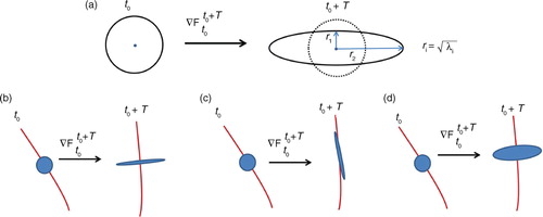
with the superscript ′ referring to matrix transposition. The finite-time Lyapunov exponent for the trajectory x (t, t ₀, x ₀) is defined from the largest eigenvalue (λ _max ) of the right Cauchy–Green strain tensor that monitors deformation in the flow field (Haller 2001, 2015). Since gives the magnitude of the largest stretching (Fig. 2a), FTLE is defined as4

Fig. 2  (a) Illustration of the deformation of a unit circle between t ₀ and t ₀+T; r ₁ and r ₂ represents the stretching in the lowest and the largest stretching directions, respectively. Schematic representation of the effects of (b) normal repulsion (incompressible case), (c) shear (incompressible case) and (d) divergence-dominated (compressible case) FTLE ridges on their close neighbourhood.

Positive values indicate stretching and negative values indicate contraction, which can only occur in compressible flows, and are useful for identifying trapping regions (Perez-Munuzuri 2014). Of particular interest are maxima in the FTLE fields, known as FTLE ridges, which capture regions of maximal stretching such as would be expected near the BG periphery.

LAD, shear and hyperbolic structures

In incompressible flow, stretching about a material line can be due to normal expansion, which is usually associated with hyperbolic structures, or tangential expansion which is associated with shear. Additionally, in a compressible case like the ice-drift field, stretching can be due to divergence. Since FTLEs hide these differences, it is necessary to further investigate the ridges for a more detailed understanding of the flow. In order to distinguish between relative contributions of divergence, shear and hyperbolic structures to high FTLEs, we first introduce LAD. We know that5 where λ ₁ and λ ₂ are the smaller and larger eigenvalues of the right Cauchy–Green strain tensor, respectively.

Following Liouville's theorem (Arnold 1978):6 Equations 3, 5 and 6 yield7 After some algebraic transformation, we get

According to Eqn. 8, LAD is directly computable from the eigenvalues of the . If LAD is small on an FTLE ridge, then the high FTLE values are due to shear or normal repulsion. To distinguish these phenomena, we recall Theorem 3 of Haller (2002) which states that the FTLE ridge is a hyperbolic material line at the point x ₀ at t ₀ if9 where e _n ( x ₀, t ₀) is a unit vector which is normal to the FTLE surface and S ( x ₀, t ₀) is the rate-of-strain tensor, the symmetric part of the velocity gradient tensor, Eqn. 9, has been evaluated in the divergence-free part of the velocity field which was obtained by discrete Hodge–Helmholtz decomposition (Guo et al. 2005).

The contribution of shear/normal repulsion and divergence was determined according to the ratio between the eigenvalues of the Cauchy–Green strain tensor. The divergence can be seen as an isotropic (directionless) stretching; we call a ridge divergence-dominated if this isotropic stretching starts to dominate over the attraction, which would be due to incompressibility in the direction of the lowest stretching. Technically, the ridge is divergence-dominated according to the criterion , which geometrically would mean that the area of an initial unit circle expand to at least double its value as a result of divergence.

This distinction identifies the properties and the behaviour of the ridges over the investigated finite time interval. For a hyperbolic ridge stretching occurs perpendicular to the ridge with negligible contribution from divergence (Fig. 2b); for a shear ridge stretching occurs along the ridge (Fig. 2c); and for divergence the whole material surface repels in the perpendicular direction (Fig. 2d). Note that hyperbolic structures can exist in incompressible flows as opposed to divergence-generated ones. Although this is a commonly used classification in non-linear dynamical systems theory, we found that FTLE ridges do not provide a signature of hyperbolic material lines or normal repulsion in the ice-drift field for the space and timescales considered. Furthermore, we found that the Eulerian stagnation points in the ice-drift field move quickly with respect to the particles; in such a field obtaining noteworthy (influential) hyperbolic structures is unlikely according to Haller & Poje (1998).

Shear ridges and divergence are, however, observed for the time frame considered. The absence of hyperbolic features may be due to the fact that at minimum a continuous two-year integration time frame is required to capture recirculation of sea ice in the BG, as demonstrated in recent back-trajectory analyses in observational sea-ice thickness studies by Renner et al. (2014). Since summer data are not provided for the OSI SAF data set, only a six-month integration interval is available.

Data

FTLE fields were computed using the low-resolution sea-ice drift product from the EUMSTAT OSI SAF High Latitude Processing Centre. OSI SAF ice motion vectors are estimated by an advanced cross-correlation method—the Continuous Maximum Cross Correlation Method—on pairs of satellite images over two-day intervals (Lavergne et al. 2010). Low-resolution ice-drift data sets are computed daily from aggregated maps of passive microwave (SSMIS, SSM/I, AMSR-E) or scatterometer (ASCAT) signals. In the present study, we use the merged (multi-sensor) data set that combines single-sensor products and provides continuous spatial coverage of daily ice-drift fields. As a result, 48-h global ice-drift vectors at a spatial resolution of 62.5 km on a polar stereographic grid are available for fall, winter and spring—that is, from October to May—from 2006 to 2014.

Results and discussion

Distinct dynamical regions defined by FTLEs

FTLEs measure the deformation for a certain integration time with respect to the initial configuration. FTLE fields for the integrated November–April time frame from 2006 to 2014 illustrate three distinct regions characterized by strong deformation (red filaments) for all winters (Fig. 3). These three regions and persistent features include FTLE ridges that: (i) extend from the western Beaufort Sea to the East Siberian Sea; (ii) exist close to Banks Island and eastern Beaufort Sea; and (iii) exist in those regions of the central Arctic from which the ice parcels are advected close to Fram Strait during the investigated period.

Fig. 3  Spatial distribution of FTLE [1/day] fields from 2006 to 2014 based on OSI SAF sea-ice drift data. FTLE ridges (red filaments) indicate the initial location of particles that experience maximal stretching during the November to May integration time frame.

Advected FTLE fields, which demonstrate evolution in these distinct features from November to the end of April (Fig. 4), show that the FTLE ridges extending from the western Beaufort Sea to the East Siberian Sea are advected poleward in a manner that coincides spatially with the Northwind Ridge. It should be noted that FTLE ridges (Fig. 4a, left panels) indicate initial locations of ice which will experience maximum stretching during the investigated time period, whereas the advected FTLE map shows where they were transported to the end of April. Advected FTLE ridges in the western Beaufort Sea may further provide a signature of the enhanced geostrophic currents at the BG periphery noted by McPhee (2013).

Fig. 4  (a) FTLE [1/day] and advected FTLE field. The left-hand panels show FTLE features identified for the November to May integration time; the right-hand panels demonstrate the positions of the features at 1 May. (b) Average FTLE field from 2006 to 2014 highlighting the three persistent and distinct dynamical features/regions associated with maximum deformation, in addition to weak and negative FTLEs in the central Arctic that depict convergence in the compressible ice-drift field. Blue arrows represent the schematic motion of the features during the integration time.

The FTLE ridge to the west of Banks Island is stretched as it is transported by the anticyclonic circulation of the BG to the southern Beaufort Sea. FTLE ridges in the central Arctic are also deformed as they are transported through Fram Strait by the TDS.

Averaged FTLE fields for 2006–2014 (Fig. 4b) depict the aforementioned three distinct dynamical regions with strong deformation. The first and second distinct features were highlighted by Herman & Glowacki (2012) as regions where the probability of extreme deformation events is the highest, based on the statistical analysis of 594 satellite-derived sea-ice deformation maps provided by the RADARSAT Geophysical Processor Systems. Whereas such studies highlight regions of strong deformation based on an Eulerian assessment, the present approach, which is based on a Lagrangian interpretation, highlights temporal evolution in these features. For the timescales considered, particles initially released in the Beaufort Sea region and western Arctic remain and experience strong deformation within the western Arctic, and align with the Northwind Ridge. By contrast, particles initially released in the central Arctic are advected along the northern coast of Greenland through Fram Strait. Further investigation of the trajectories shows that the FTLE ridges in the central Arctic anticipate and provide a signature of large deformation through Fram Strait (feature 3; Fig. 4b). Weak and negative FTLEs (convergence) are observed in the rest of the central Arctic and north of the Laptev Sea. It should be noted that in forward time analysis negative FTLEs cannot occur in incompressible flows, because it would mean that the material shrinks in each directions which cannot be area preserving. Therefore, negative FTLEs always show convergence due to compressibility.

Spatial variability of shear and divergence

In order to determine whether the FTLE ridges provide a signature of large deformation due to shear or divergence, the components of LAD outlined in Eqn. 8 are investigated for all years, and the results for the 2007, 2008 and 2012 winters presented (Fig. 5). Regional comparisons for all years indicate that ice deformation in the Beaufort Sea region is governed primarily by divergence and the central Arctic by shear. Specifically, the Beaufort Sea region is governed by high LAD in 2007 and 2008; the former is consistent with results found by Kwok & Cunningham (2011) using RADARSAT imagery and Geophysical Processor Systems data, showing sea-ice deformation in November and December of 2007 to be governed by strong (cumulative) divergence. Divergence-dominated FTLE ridges in the Beaufort Sea also provide a signature of fractures, Ekman pumping and increased local mixing characteristic of changes in ice dynamics detected in this region (Yang 2006, 2009; McPhee 2013; Timmermans et al. 2014). Furthermore, the large convergence zone (orange rectangle in Fig. 5) characteristic of ridging north of the Canadian Arctic Archipelago was also measured/found by Kwok & Cunningham (2011).

Fig. 5  (a) FTLE [1/day] fields, (b) corresponding LAD [1/day] fields (Eqn. 8) and (c) shear and divergence-dominated FTLE ridges for 2007, 2008 and 2012 winters. The red circle highlights the region of strong divergence in the Beaufort Sea, and the orange rectangle the region of convergence north of the Canadian Arctic Archipelago in 2007, both of which are documented in Kwok & Cunningham (2011). Shear- and divergence-dominated FTLE ridges capture spatial variability and relative contributions of both to deformation, while also indicating increased prevalence in divergence in 2012–2013.

From 2006 to 2014, the central Arctic is governed by shear; since 2011 FTLE ridges in this region have been governed by both shear and divergence, in a manner consistent with faster drift and loss of MYI in the TDS (Kwok et al. 2013) and a continued decline in TDS sea-ice thickness, as described in Renner et al. (2014). Smaller-scale, divergence-dominated FTLE ridges throughout the Arctic (Figs. 3, 5c) in 2012 further highlight increased localization in dispersion characteristic of mixing following the record minimum in summertime sea-ice extent.

Connection between MYI and FTLEs

Significant loss of MYI, most notably in the Pacific Sector of the Arctic, is one of the more striking signatures of changes in the Arctic sea-ice cover (Maslanik et al. 2011). Comparison of composite FTLE PDFs for higher (2006, 2009 and 2010) and for lower (2007 and 2008) MYI years (identified from Maslanik et al. [2011] for the 2006–2011 time frame) captures correspondence between high FTLEs and lower MYI regimes (Fig. 6a).

Fig. 6  (a) PDFs of FTLE [1/day] fields in the Arctic for high (2006, 2009, 2010) and low (2007, 2008) MYI years defined following Maslanik (2011). (b) PDFs of FTLE [1/day] fields for high and low MYI years as in (a), yet for the Beaufort Sea region only. Maximum FTLEs (ridges) for (c) 2006–2011 and (d) 2012 highlighting the emergence of ridges in the central Arctic and increased localization in dispersion.

Higher FTLE values are more prevalent for low MYI years, as evidenced in the PDF tails. This behaviour is amplified in the Beaufort Sea region (Fig. 6b) during low MYI years, where loss of perennial ice (Barber et al. 2009; Krishfield et al. 2014) and enhanced geostrophic currents (McPhee 2013) are manifested in a distinct shift in the FTLE PDF to higher values characteristic of increased deformation associated with the emergence of younger and more mobile ice.

Evident also in the FTLE fields is increased localization of the FTLE ridges following the 2012 record in minimum sea-ice extent: more numerous and smaller ridges are observed throughout the Arctic, especially in the central Arctic in 2012 and a lesser extent in 2013 (Fig. 6c). Comparison of maximum FTLE field 2006–2011 and FTLE field 2012 shows that there is a unique area in the central Arctic (highlighted by dashed circles in Fig. 6c, d) where previously unobserved FTLE ridges appear. This observation provides evidence for a dispersion regime characterized by local dynamics and mixing after the summer of 2012.

Conclusions

In this study, FTLEs are presented as a new diagnostic to examine spatiotemporal changes in large-scale sea-ice drift and deformation in the Arctic. In addition to results shown to be consistent with earlier studies, including the existence of three distinct dynamical regions associated with enhanced stretching and deformation rates, new features emerge in both the FTLE and advected FTLE fields.

Analysis of LAD and FTLE fields indicate that the Beaufort Sea region is governed primarily by divergence and Fram Strait by shear. Increased contributions from divergence in 2012 provide a signature of increased mixing throughout the central Arctic. Increased localization in the FTLE features evident in more numerous and smaller FTLE ridges in 2012 further indicates a transition to a dynamical regime characterized by dynamics on a local scale and dispersion. This is further demonstrated in FTLE PDFs for low and high MYI years, showing higher FTLEs during years with lower MYI extent, particularly in the Beaufort Sea region. The results from this analysis demonstrate the ability of FTLEs to capture, in contrast to previous Eulerian studies, the evolution in shear- and divergence-dominated regions of maximal stretching. FTLEs further capture a transition to enhanced deformation rates and mixing evident following the 2012 record in summertime minimum sea-ice extent, with implications for pollutant and contaminant transport within an increasingly mobile and weaker ice cover in the Arctic.

Acknowledgements

The authors would like to thank Professor George Haller for helpful advice and suggestions, and for facilitating this study. The authors would also like to thank two anonymous reviewers for their helpful advices. SS was funded by the Scientific Exchange Programme (project code 13.073). DGB was funded by the Canadian Networks of Centres of Excellence program and a Canada Research Chairs grant. The authors thank OSI SAF for providing sea-ice motion data.

References

- Arnold V.I. Mathematical methods of classical mechanics. 1978; New York: Springer.
- Barber D.G., Galley R., Asplin M.G., De Abreu R., Warner K., Pucko M., Gupta M., Prinsenberg S., Julien S. Perennial pack ice in the southern Beaufort Sea was not as it appeared in the summer of 2009. Geophysical Research Letters. 2009; 36: 24501. http://dx.doi.org/10.1029/2009GL041434.
- Comiso J.C., Hall D.K. Climate trends in the Arctic as observed from space. Wiley Interdisciplinary Reviews: Climate Change. 2014; 5: 389–409.
- Fowler C., Emery W., Maslanik J.A. Satellite-derived evolution of Arctic sea ice age: October 1978 to March 2003. IEEE Geoscience and Remote Sensing Letters. 2003; 1: 71–74.
- Guo Q., Mandal M., Li M. Efficient Hodge-Helmholtz decomposition of motion fields. Pattern Recognition Letters. 2005; 26: 493–501.
- Hakkinen S., Proshutinsky A., Ashik I. Sea ice drift in the Arctic since the 1950s. Geophysical Research Letters. 2008; 35: 19704. http://dx.doi.org/10.1029/2008GL034791.
- Haller G. Distinguished material surfaces and coherent structures in three-dimensional fluid flows. Physica D. 2001; 149: 248–277.
- Haller G. Lagrangian coherent structures from approximate velocity data. Physics of Fluids. 2002; 14: 1851–1861.
- Haller G. Lagrangian coherent structures. Annual Review of Fluid Mechanics. 2015; 47: 137–162.
- Haller G., Poje A. Finite-time transport in aperiodic flows. Physica D. 1998; 119: 352–380.
- Haller G., Yuan G. Lagrangian coherent structures and mixing in two dimensional turbulence. Physica D. 2000; 147: 352–370.
- Herman A., Glowacki O. Variability of sea ice deformation rates in the Arctic and their relationship with basin-scale wind forcing. The Cryosphere. 2012; 6: 1553–1559.
- Hutchings J.K., Rigor I.G. Role of ice dynamics in anomalous ice conditions in the Beaufort Sea during 2006 and 2007. Journal of Geophysical Research—Oceans. 2012; 117: 00E04. http://dx.doi.org/10.1029/2011JC007182.
- Hutchings J.K., Roberts A., Geiger C., Richter-Menge J. Spatial and temporal characterization of sea-ice deformation. Annals of Glaciology. 2011; 52: 360–368.
- Krishfield R.A., Proshutinsky A., Tateyama K., Williams W.J., Carmack E.C., McLaughlin F.A., Timmermans M.L. Deterioration of perennial sea ice in the Beaufort Gyre from 2003 to 2012 and its impact on the oceanic freshwater cycle. Journal of Geophysical Research—Oceans. 2014; 119: 1271–1305.
- Kwok R., Cunningham G.F. Deformation of the Arctic Ocean ice cover after the 2007 record minimum in summer ice extent. Cold Regions Science and Technology. 2011; 76/77: 17–23.
- Kwok R., Spreen G., Pang S. Arctic sea ice circulation and drift speed: decadal trends and ocean currents. Journal of Geophysical Research—Oceans. 2013; 118: 2408–2425.
- Lavergne T., Eastwood S., Teffah Z., Schyberg H., Breivik L.-A. Sea ice motion from low resolution satellite sensors: an alternative method and its validation in the Arctic. Journal of Geophysical Research—Oceans. 2010; 115: 10032. http://dx.doi.org/10.1029/2009JC005958.
- Lichtenberg A.J., Lieberman M.A. Regular and chaotic dynamics. 1992; New York: Springer.
- Maslanik J., Stroeve J., Fowler C., Emery W. Distribution and trends in Arctic sea ice age through spring 2011. Geophysical Research Letters. 2011; 38: 13502. http://dx.doi.org/10.1029/2011GL047735.
- McPhee M. Intensification of geostrophic currents in the Canada Basin, Arctic Ocean. Journal of Climate. 2013; 26: 3130–3138.
- Peacock T., Haller G. Lagrangian coherent structures: the hidden skeleton of fluid flows. Physics Today. 2013; 66: 41–47.
- Perez-Munuzuri V. Mixing and clustering in compressible chaotic stirred flows. Physical Review E 89. 2014; 022917. http://dx.doi.org/10.1103/PhysRevE.89.022917.
- Rampal P., Weiss J., Marsan D. Positive trend in the mean speed and deformation rate of Arctic sea ice. Journal of Geophysical Research—Oceans. 2009; 113: 03002. http://dx.doi.org/10.1029/2007JC004143.
- Rampal P., Weiss J., Marsan D., Lindsay R., Stern H. Scaling properties of sea ice deformation from buoy dispersion analysis, 1979–2007. Journal of Geophysical Research—Oceans. 2008; 114: 05013. http://dx.doi.org/10.1029/2008JC005066.
- Renner A.H.H., Gerland S., Haas C., Spreen G., Beckers J.F., Hansen E., Nicolaus M., Goodwin H. Evidence of Arctic sea ice thinning from direct observations. Geophysical Research Letters. 2014; 41: 5029–5036.
- Rigor I.G., Wallace J.M. Variations in the age of Arctic sea ice and summer sea-ice extent. Geophysical Research Letters. 2004; 31: 09401. http://dx.doi.org/10.1029/2004GL019492.
- Spreen G., Kwok R., Menemenlis D. Trends in Arctic sea ice drift and role of wind forcing: 1992–2009. Geophysical Research Letters. 2011; 38: 19501. http://dx.doi.org/10.1029/2011GL048970.
- Stroeve J.C., Maslanik J.A., Serreze M.C., Rigor I., Meier W., Fowler C. Sea ice response to an extreme negative phase of the Arctic Oscillation during winter 2009/2010. Geophysical Research Letters. 2011; 38: 02502. http://dx.doi.org/10.1029/2010GL045662.
- Thorndike A.S. Untersteiner N. Kinematics of sea ice. The geophysics of sea ice. 1986a; New York: Springer. 489–549.
- Thorndike A.S. Diffusion of sea ice. Journal of Geophysical Research—Oceans. 1986b; 91: 7691–7696.
- Timmermans M.-L., Proshutinsky A., Golubeva E., Jackson J.M., Krishfield R., McCall M., Platov G., Toole J., Williams W., Kikuchi T., Nishinom S. Mechanisms of Pacific Summer Water variability in the Arctic's Central Canada Basin. Journal of Geophysical Research—Oceans. 2014; 119: 7523–7548.
- Weiss J. Drift, deformation and fracture of sea ice—a perspective across scales. 2013; Dordrecht: Springer.
- Yang J. The seasonal variability of the Arctic Ocean Ekman transport and its role in the mixed layer heat and salt fluxes. Journal of Climate. 2006; 19: 5366–5387.
- Yang J. Seasonal and interannual variability of downwelling in the Beaufort Sea. Journal of Geophysical Research—Oceans. 2009; 114: 0014. http://dx.doi.org/10.1029/2008JC005084.