Power laws and inverse motion modelling: application to turbulence measurements from satellite images

Abstract

In the context of tackling the ill-posed inverse problem of motion estimation from image sequences, we propose to introduce prior knowledge on flow regularity given by turbulence statistical models. Prior regularity is formalised using turbulence power laws describing statistically self-similar structure of motion increments across scales. The motion estimation method minimises the error of an image observation model while constraining second-order structure function to behave as a power law within a prescribed range. Thanks to a Bayesian modelling framework, the motion estimation method is able to jointly infer the most likely power law directly from image data. The method is assessed on velocity fields of 2-D or quasi-2-D flows. Estimation accuracy is first evaluated on a synthetic image sequence of homogeneous and isotropic 2-D turbulence. Results obtained with the approach based on physics of fluids outperform state-of-the-art. Then, the method analyses atmospheric turbulence using a real meteorological image sequence. Selecting the most likely power law model enables the recovery of physical quantities, which are of major interest for turbulence atmospheric characterisation. In particular, from meteorological images we are able to estimate energy and enstrophy fluxes of turbulent cascades, which are in agreement with previous in situ measurements.

• image assimilation
• atmospheric turbulence
• Bayesian inference
• motion structure functions
• power-laws
• energy flux

1. Introduction

Images constitute important data for studying geophysical flows since they can characterise a large range of spatial scales in comparison to sparse information provided by standard point measurement techniques.

Correlation-based techniques are common inverse approaches to extract sparse velocity fields from image sequences. These methods penalise deviations from constant flows over a spatial window and from the brightness preservation of the tracer along its trajectory (Leese et al., 1971). Such methods have demonstrated their robustness and accuracy for velocity measurement in experimental studies (Adrian, 1991). However, correlation is not a physical-based image observation model and is particularly limited in the context of geophysical flows (e.g., because of small-scale intermittency and 3-D effects). Moreover, the assumption of local constant motion gives rise to an intrinsic measurement scale associated to the correlation window size and an artificial regularity of the flow. In particular, for low-contrast observations such as satellite images, correlation-based methods are considerably limited and provide only very sparse motion fields.

In computer vision, estimating the projected apparent motion of a 3-D scene onto the image plane, referred in the literature as optical flow, has been an intensive subject of research since the 1980s and the work of Horn and Schunck (1981). The inverse motion modelling proposed in this seminal work is formulated in a differential framework enabling the easy introduction of a physical-based direct observation model (relying on brightness preservation, mass conservation, scalar transport, etc.) adapted to the particular image data at hand (Fitzpatrick, 1988; Heas et al., 2007a; Heas and Memin, 2008; Liu and Shen, 2008). The model links the motion field to the image intensity function. However, these models are insufficient for fluid flow estimation since they are ill conditioned, as they are generally constituted at each point of a scalar equation for two unknowns. The introduction of regularization constraints is required to remove the motion ambiguities and achieve inversion. Common spatial regularizers may introduce measurement inaccuracy since they impose in a small spatial neighbourhood a prior smoothness, which may improperly describe the regularity followed by fluid flows. Moreover, they strongly depend on a tuning parameter weighting the amount of smoothing required to cure the ill-posed nature of the inverse motion problem. For large values of this parameter (which is almost unavoidable when facing noisy images or with low photometric contrast), the solution tends to be too smooth and presents sometimes lack of accuracy at large scales. Alternatively, dynamical constraints embedded in variational assimilation frameworks have recently been proposed for geophysical flow estimation (Papadakis and Memin, 2008; Corpetti et al., 2009). Unfortunately, these methods rely only on a large-scale dynamical model, which is not valid at the pixel level.

This work aims at showing the possibilities to alleviate these limitations in coupling two main ingredients: turbulence statistical modelling and Bayesian inference. In the one hand, important advances have been done in the statistical modelling of turbulence since the precursor work of Kolmogorov in 1941 (see, e.g., Kraichnan, 1967; Frisch, 1995; Kurien et al., 2000; Falkovich et al., 2001; Lindborg and Cho, 2001). In particular, it has been shown from the Navier–Stokes equations for different flows that turbulent motion regularity can be characterised using some (assumed universal) scaling properties of the probability distribution function (PDF) of motion increments. On the other hand, Bayesian modelling enables the reconstruction of complex physical processes in the presence of incomplete observations and prior geophysical scaling (Berliner et al., 1999; Wikle et al., 2001; Hoar et al., 2003). Moreover, this framework results in the design of non-parametrical methods and provides reliable model selection tools given some data (Gull, 1989; MacKay, 1992; Jaynes, 2003; Robert, 2007).

To be more precise, in this work we propose a method for motion estimation and turbulence characterisation, which exploits simultaneously two ideas: (1) the use of turbulence scaling laws for motion regularization in optic-flow inverse problems and (2) the selection by Bayesian evidence maximisation of the most appropriate power law model describing the image intensity function. The resulting frame-to-frame regularization is built from the physics of fluids and involves neither dynamical constraints nor an adjoint model within a variational assimilation framework. It is intrinsically multi-scale as it controls the solutions within a prescribed scale range. It is also non-parametric in the sense that it does not involve the tuning of any smoothing parameters. Finally, it allows as a by product the recovery of some important quantities for turbulence characterisation such as energy flux across scales.

After validating the method using synthetic images from numerical simulations of 2-D turbulence, we use the proposed regularization model to analyse data from meteorological image sequences. Recovered atmospheric quantities such as the energy and enstrophy flux are shown to be in good agreement with in situ measurements. Moreover, reconstructed second- and third-order structure functions and PDFs of velocity increments are consistent with previous analysis using aircraft data (Lindborg, 1999; Lindborg and Cho, 2001). We believe that those first results demonstrate the potential of image-based techniques in complementing other measurements for geophysical studies.

The study is organised as follows. In Section 2, we briefly overview optic-flow methods and review the motion scaling properties developed in theoretical works on turbulence. In Section 3, self-similar regularizers are briefly introduced. Finally, the synthetic and real-world experiments on meteorological image data are presented, followed by the conclusions. Details of the model, of the multi-scale constraint minimisation problem and of the use of Bayesian evidence for the optimal selection of the prior self-similar model are given in the Appendices.

2. Related work

2.1. Optic-flow methods

This section briefly describes some solutions for the computation of velocity fields from image sequences. Interested readers may refer to an extended review (Heitz et al., 2010) for a more complete account of different techniques proposed in the literature and the description of some new trends based on variational assimilation processes.

2.1.1. Image observation model.

Motion perceived through image intensity I(x, t) variations and the projection on the image plane of the velocity field v=(u, v ) are identical when considering rigid motion and stable lighting conditions. In this situation, motion v respects the standard optical flow constraint (OFC) equation, which reads:1 For fluids, this equation remains valid in the theoretical case of 2-D incompressible flows. This case is relevant for many geophysical applications that are quasi-2-D, e.g., in meteorology and oceanography (Pedlosky, 1987). For shallow-water flows visualised in a projected image plane, authors in Liu and Shen (2008) derived a physics-based image observation model using the scalar transport equation, which reads:2 where κ denotes a diffusion coefficient. For layered geophysical flows, based on the mass conservation principle, a non-diffusive model analogous to (2) has been proposed in the literature to link the image intensity function I to a vertically averaged horizontal velocity field v (Heas et al., 2007a; Corpetti et al., 2009). However, all these observation models remain under-constrained, as they provide only one equation for two unknowns (u, v) at each spatio-temporal location (x, t).

2.1.2. Standard regularization constraints.

To deal with this under-constrained estimation problem, an additional set of constraints have to be satisfied by the sought velocity field.

In the standard computer vision literature, dealing with frame-to-frame motion estimation in natural scenes, these constraints are usually chosen to enforce some spatial regularity of the solution. Global regularization schemes are convenient to enforce global coherence via local spatial dependencies. More precisely, estimation is performed through the minimisation of an energy function composed of two terms:3 The first term, f _d  (I, v) is the observation model also called data term. Its minimisation penalises discrepancies from the observation models. As an example, relying on the OFC equation and a quadratic penalisation results in a data term1 4 The second term, f _r (v) (the ‘regularization term’), acts as a spatial prior enforcing the solution to follow some smoothness properties. The coefficient α (>0) is a regularization parameter that balances between smoothness and global adequacy to the observation model. In this framework, Horn and Schunck (1981) proposed a first-order regularization of spatial components u and v of velocity field v:5 However, motion gradient penalisation is not well suited for fluid flows as it penalises in a homogeneous way the curl and the divergence (Corpetti et al., 2002).

In the context of geophysical flows, second-order spatial regularizers on motion vorticity and divergence have been proposed to overcome these limitations (Corpetti et al., 2002; Yuan et al., 2007; Heas et al., 2007a). It is important to outline that these spatial regularization constraints do not rely on physical kinematics properties. At best they mimic qualitative regularity properties of the physical system of interest, i.e., coherent blobs of vorticity and divergence. Recently, Corpetti et al. (2009) proposed to rely on large-scale dynamical constraints enforcing the temporal coherence of the solution, since in geophysics there exist some fair approximations of the physical equations governing the flows. The authors introduced a 4-D variational assimilation technique to solve the motion estimation problem on a whole image sequence subject to layered shallow-water dynamical constraints. Unfortunately, this choice of constraints does not entirely remove the under-determination of the estimation problem and still yields an infinite set of solutions. To close the problem, Corpetti et al. (2009) needed to rely on an additional local spatial regularization on motion measurements (Lucas and Kanade, 1981) in consistency with a filtered version of shallow-water dynamics. By doing so, they restricted themselves to the determination of the solution at large scales (on a grid of a 100 km resolution).

In summary, in frame-to-frame estimation or variational image assimilation, there is actually a lack of physical constraints to solve at small scales the under-constrained fluid motion estimation problem. However, as we will show in the following, turbulence statistical models can provide the needed closure.

2.2. Turbulence statistical modelling

Since experimental results at the beginning of the 20th-century, and later Kolmogorov's theoretical works, turbulent motion increments have been known to be structured as scale invariant spatial processes. In many turbulence models, a quantity of interest is the longitudinal velocity increment, which, in the direction of a unitary vector n _θ, is given by6 where the scalar represents a spatial increment. In turbulent studies, homogeneity and isotropy are often assumed; that is to say, it is considered that statistical properties of the velocity field are invariant under translation of spatial location x and rotation of direction n _θ.2 Consistently with these assumptions, the dependence on x and θ can be dropped and moments of order p of the PDF of velocity increments can be approached by spatial integration:7 in two dimensions, and where ∣Ω∣ denotes the spatial domain area. S _p (ℓ) are the so-called longitudinal structure functions.

For 3-D isotropic turbulent flows, Kolmogorov (1941) demonstrated from the Navier–Stokes equations that the third-order moment of the PDF , namely the third-order structure function, is linear w.r.t. scale and follows the well-known ‘4/5 law’: in the inertial range (see, e.g., Frisch (1995) for details on this demonstration). The inertial range is defined as the range of scales [η, ℓ₀], where η represents the largest molecular dissipative scale and where ℓ₀ is smaller than the diameter L of the largest vortex. Within this range, an energy flux cascades from large to small scales. The kinetic energy dissipation rate corresponds to this energy flux passed across scales which is then evacuated at small scales by molecular viscosity.

Analogously, for pure 2-D turbulence with energy injection at scale ℓ₀, Kraichnan (1967) demonstrated that two different cascades are coexisting: a direct cascade of enstrophy (the L ² norm of the vorticity ω=∇×v), which satisfies within the inertial range [η, ℓ₀], and an inverse cascade of energy where within the range [ℓ_0, L]. An enstrophy flux ɛ _ω passes in the direct cascade from large to small scales, whereas an energy flux ɛ passes in the inverse cascade from small to large scales.

In the case of atmospheric turbulence, the actual scaling laws constitute still open questions. Lindborg (1999) and Lindborg and Cho (2001) consider scaling laws inferred from aircraft measurements and propose an answer to the question: ‘can atmospheric flow statistics be explained by two-dimensional turbulence?’. The authors showed that, under some isotropy assumption, the self-similar processes observed in the aircraft data (Nastrom et al., 1984) at small and at large scales can be modelled by the superposition of a 3-D direct energy cascade and a 2-D direct enstrophy cascade so that8 Aside from the problems to determine direction of energy and enstrophy cascades in atmospheric turbulence, it should be mentioned that there are still several independent exact relations that hold for the third-order structure function and which predict power law behaviour for several flows of interest in atmospheric sciences (Monin and Yaglom, 1975; Kurien et al., 2000).

Going further, Kolmogorov assumed that the longitudinal velocity increments were strictly self-similar to explain the scaling laws observed in many experiments. If this is true, the normalised PDF of motion increments is self-similar through scales. This implies that, in a given cascade, the pth order structure function follows a power law:9 with universal exponents ζ _p depending on space dimension, and where the prefactors γ _p are a function of energy flux ɛ (or enstrophy flux ɛ _ω in two dimensions). A corollary of the strictly self-similar assumption is that in inertial range any 3-D turbulent flow has a uniform Lipschitz regularity of ζ₁=1/3, while a 2-D turbulent flow is characterised by ζ₁=1 (i.e., it is regular). However, it is now well known that for 3-D turbulence and for the direct cascade range of 2-D turbulence, the Kolmogorov assumption deviates from reality because of intermittency (tendency of the flow to develop strong gradients at small scales). As a consequence, only non-strict self-similarity can in reality be assumed. It results that deviations on exponent values can be expected for , although power law behaviour in inertial range still holds. The special case of the inverse cascade of 2-D turbulence must be remarked, as growing evidence indicates that it is self-similar (Benzi and Scardovelli, 1995; Bernard et al., 2006).

Finally, another result that is used in the following sections is that any 2-D or 3-D turbulent flow is regular in the dissipative range; using Taylor expansion we then have within ℓ∈[0, η]. All these general power law dependencies motivate the use of self-similar priors for motion estimation as discussed in the next section.

3. Regularization of motion increments

Exhibiting self-similarity properties of fluid flows enables to define prior spatial regularization functionals. Besides providing a closure for motion estimation, power law priors have several advantages compared with traditional smoothing functions: they constitute physical sound regularizers for fluid motion and they provide intrinsic multi-scale prior models, which structures motion across scales. In this section, we discuss the use of the self-similar regularization of motion increments with a prior power law and postpone to Section 4 how Bayesian modelling is used to select the most appropriate power law from the images (instead of imposing one).

3.1. Self-similar constraints

Let us first formalise the use of self-similar constraints to specify regularization functionals. Although there is no exact prediction on its scaling law for non-strictly self-similar flows, we chose to use the second-order structure function S ₂(ℓ) because it constitutes a convenient quadratic constraint for our purpose. Also, this quantity is related with the energy spectrum and the two-point correlation function, quantities of interest in experiments and simulations. Since the exponent of the power law is unknown, we take into account in Section 4 deviations from the predicted laws by selecting the most likely power law defined by the two parameters γ₂ and ζ₂ given the image data (γ and ζ for simplicity in the following).

S ₂(ℓ) is an expectation which can be obtained by spatial integration over the image domain and over all directions as presented in eq. (7). A self-similar constraint is then defined at each scale ℓ as the difference between the second-order structure function and (for the moment) a given power law depending on some parameters γ and ζ:10 An estimated motion field should thus respect the self-similar constraint:11 This constraint replaces the usual smoothness constraints used in the minimisation problem discussed in Section 2.1.

3.2. Constrained motion estimation problem

Referring to Section 2.1, the minimisation of the ill-conditioned optic-flow estimation problem can be written as12 Adding the self-similar constraints, we obtain the closed constraint optic-flow minimisation problem:13 where I is the scale range of the given power law. The system (13) is discretized on a discrete set of scales, and the velocity field is recovered from the image intensity solving the constrained minimisation using the Lagrangian formalism. It yields the optimal solution:14 where the Lagrangian function is given by and where represents the Lagrangian multipliers. Further details are given in Appendix A.

4. Selection of a prior power law

So far, the proposed model recovers motion from images conditioned by some prior power law model for the second-order structure function. This power law can be given by turbulence statistical models describing the self-similar structure of turbulence, which is assumed universal in the works of Kolmogorov (1941), Kraichnan (1967) and Lindborg and Cho (2001). However, we now want to relax this universal assumption by allowing ζ and γ to change and select the most appropriate power law model for motion estimation given only the image data. With this prior model selection, we cope with uncertainties in turbulence theoretical predictions associated to, e.g., intermittency effects. Moreover, it will enable us to reveal directly from the images important physical quantities in turbulence such as power law exponents, flux across scales, or energy and enstrophy dissipation rates. To this end, we now reformulate the constrained motion estimation problem in a probabilistic framework, and we show how probability of the prior model can be evaluated given image data. Bayes’ rule provides a nice framework to evaluate this model probability.

4.1. Probabilistic model

A probabilistic reformulation of the global motion estimation problem yields a model relating the image intensity function variable I, the motion field variable v, an observation model variance and, finally, a prior power law model . Noticing conditional independences, the joint probability can be factorised in three primary statistical models yielding the Bayesian hierarchical model:15 where represents the image observation PDF or likelihood, denotes the motion prior PDF and and denote the prior PDF, respectively, on the likelihood hyper-parameter and the power law model. Let us note that Bayesian hierarchical model can also be used to decompose multi-dimensional probability distributions of complex spatio-temporal processes in geophysics (Berliner et al., 1999; Wikle et al., 2001; Hoar et al., 2003). Using hierarchical models, it is then possible to infer the joint maximum a posteriori (MAP) estimate by maximisation of the joint probability w.r.t. v, β and . However, it is well-known in Bayesian analysis that selection with a joint MAP estimator tends to over-fit the data, i.e., to favour models with large degrees of freedom (Robert, 2007). Bayesian analysis suggests to rely instead on marginalised posterior distributions for model and hyper-parameter selection. Therefore, by successive marginalisation of the joint posterior distribution , we perform three levels of inference yielding estimates: (1) the velocity field; (2) the variance of the observation model error; and (3) the power law model. Although, variable β does not affect the first level of inference, we will see that it is necessary to consider the variance of the observation model to perform model selection. In the following for notational convenience, the dependence of the Lagrangian multipliers to model will be omitted. The three levels are detailed in the next sections.

4.2. First inference level: motion field estimation

In this first level of inference, we consider the maximisation of the joint probability w.r.t. v given some data realisation I ₀, the hyper-parameter estimate and the selected scaling model :We obtain the MAP estimate . Let us show that solving the problem introduced in the previous section is equivalent to inferring a velocity field according to an MAP criterion. This can be shown using Bayes’ relation to define the motion field posterior PDF: 16 where the likelihood, the prior and the posterior are Gibbs PDF. More precisely, the quadratic observation model f _d represents the energy of an uncorrelated Gaussian likelihood PDF with constant variance β ⁻¹:17 where denotes a normalisation constant also called partition function. The constraints weighted by inverse variances form the energy of a multi-scale prior PDF:18 where denotes the partition function. At the point λ*, the Lagrangian function thus defines, up to a multiplicative factor, the energy of the posterior PDF:19 where Z _L (β, ) denotes the associated partition function. It is now obvious that the maximum v* of the posterior is reached at the minimum of the Lagrangian:20 which constitutes also the solution (14) of the constrained motion estimation problem presented in Section 3.2.

4.3. Second inference level: estimation of observation model variance

A second level of inference considers the maximisation w.r.t. β of the joint posterior PDF, marginalised over v, given the data realisation I ₀ and the selected scaling model :yielding the hyper-parameter estimate . Using again Bayes’ relation one can write:21 Assuming a flat prior on variables β, the MAP of (21) is simply the maximum likelihood (ML) estimate, or in other words the maximum of the evidence PDF . This probability is defined by a marginalisation w.r.t. the velocity field:22 Let us recall that the evidence is also the normalisation constant (w.r.t. velocity field v), which has been ignored in the first level of inference (eq. 16). Therefore, we can rewrite the evidence as a partition function ratio:23 Assuming the energy of the evidence is convex (at least locally), the variance estimate maximising the evidence is obtained by cancelling out its derivative.24 The analytical expression of the evidence probability, of its derivate and of the variance estimate is detailed in Appendix B.

4.4. Third inference level: selection of power law

A third level of inference considers the maximisation w.r.t. M of the joint posterior PDF, successively marginalised over v and β, given some data realisation I ₀:Again, Bayes’ relation is used to select the model:25 The data-dependent term, the likelihood for (also called evidence for ) appeared earlier as the normalisation constant of the second level of inference (eq. 21). Its evaluation implies marginalising out variable β:26 This integral (26) can be approached by Laplace's approximation and depends on the estimate as detailed in Appendix C. The model maximising the posterior probability (26) of the power law model:27 is obtained by uniform sampling in of the power law parameters .

As a result, it is important to outline that, a priori, no particular power law is imposed on the data, but rather the second-order structure function is constrained to follow some power law in some range of scales (which can be selected). If the smallest resolved scales in the images correspond to the dissipative scales of the flow, the constraint reduces to a multi-scale first-order smoothing, as in that range . This kind of smoothing function constitute a multi-scale generalisation of regularizer (5) computed with finite differences. On the other hand, if the smallest resolved scales in images are in the inertial range of the turbulent flow, the constraint gives a better representation of the physics of the problem than ad hoc regularizers. Finally, note that since laminar flows possess vanishing increments, their structure functions can be modelled with power laws with prefactors equal zero (). Appendix D shows with a toy example how the proposed methodology succeeds to recover this particular case. Therefore, the proposed methodology can be expected to improve the physical representation of the flow in turbulent cases and enforces smooth solutions if the hidden flow is smooth or laminar.

5. Numerical and experimental validation

5.1. Synthetic turbulence of horizontal velocity fields

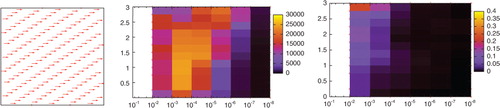
To evaluate the performance of the reconstruction of the horizontal velocity field from intensity images using the proposed self-similar regularization, synthetic image sequences were generated based on forced 2-D turbulence obtained from direct numerical simulations (DNS) of the 2-D and incompressible Navier–Stokes equations with a Reynolds number of 3000. The pseudo-spectral code used for this study solved the vorticity conservation equation and the Lagrangian equation for particle tracers transported by the flow or, in the case of scalar images, the advection–diffusion equation, i.e., model (2) in the case of divergence-free velocities, with a Pecklet number of 2100. The flow was stirred by an external force acting between wavenumbers k = 5 and 10. Figure 1 shows the isotropic (angle averaged) energy spectrum and the energy flux for one snapshot of the velocity field. A flat spectrum is observed at scales larger than the forcing scale, resulting from an incipient inverse cascade of energy. The direct cascade range shows a spectrum steeper than expected from Kraichnan phenomenology, which is not unusual in numerical simulations of 2-D turbulence and which, in this particular case, can also be associated to the moderate spatial resolution and Reynolds number considered (the slope is in fact close to –5). The simulation shows positive enstrophy flux toward small scales for wavenumbers larger than the forcing wavenumbers and a few wavenumbers with negative energy flux associated to the beginning of the inverse cascade. Also, the energy flux in the direct cascade range is negligible when compared with the enstrophy flux (see Boffetta, 2007, for examples of energy and enstrophy fluxes in high-resolution simulations of 2-D turbulence). A precise description of the simulation can be found in Carlier and Wieneke (2005). This database has proven its relevance in previous studies in the field of fluid flow estimation (Yuan et al., 2007; Heas et al., 2007b; Papadakis and Memin, 2008; Heas et al., 2009).

Fig. 1.  Isotropic energy spectrum and flux in the numerical simulation. Left: energy spectrum, as a function of the wavenumber in units of the inverse of the length of the box, and in units of 1/pixel (between parenthesis). Right: enstrophy flux (solid) and energy flux (dotted), as a function of the wavenumber using the same notation.

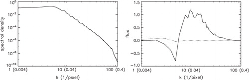
Figure 2 presents a sample of the synthetic particle and scalar images of pixels generated using the numerical simulation. The corresponding DNS velocity field is also presented in Fig. 2. The motion estimates were obtained by minimising discrepancies to the brightness consistency (1) (resp. to the scalar diffusion equation, i.e., model (2) in the case of divergence-free velocities) for particle images (resp. for scalar images) under power law constraints. The self-similar regularizer was applied only in the range of pixels (corresponding either to dissipation or to the end of the inertial range). A multi-resolution approach was used to cope with large displacements (Bergen et al., 1992). Motion estimates can be compared with the DNS motion fields and with the operational correlation-based software from LaVision company in Fig. 2. The true and reconstructed velocity fields look similar. It can also be noticed that although correlation-based methods are accurate measurement tools for particle imagery, they usually perform badly for scalar imagery. Quantitative details of the estimation are given next.

Fig. 2.  Particle and scalar images, DNS and motion estimates. From left to right: Particle (above) and scalar (below) image at time ; Turbulent motion field obtained by DNS in vectorial (above) and colour (below) representation; Motion field inferred by the proposed method and correlation-based velocity fields provided by LaVision in the context of the Fluid FET Open European project (Heitz et al., 2007) for particles (above) and scalar (below). For a better visual analysis, the velocity fields are displayed in a colour representation where colour and intensity code respectively vector orientations and magnitudes (Baker and coauthors, 2007). The corresponding colour map circle is displayed on the left.

5.1.1. Evaluation of power law selection

A flat prior was chosen on the power law parameters in (27) and, therefore, inference was performed by maximising the evidence probability (26) w.r.t. γ and ζ. This probability was evaluated by sampling the exponent κ near the theoretical value of 2 (the value expected for a dissipative range or for a direct enstrophy cascade from the theoretical predictions), and by sampling the prefactor γ around a first guest given for instance by a least square (LS) fitting of the solution of a rough Horn and Schunck (1981) estimation.

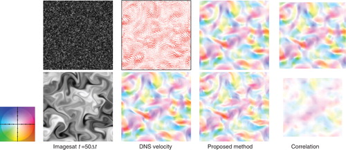
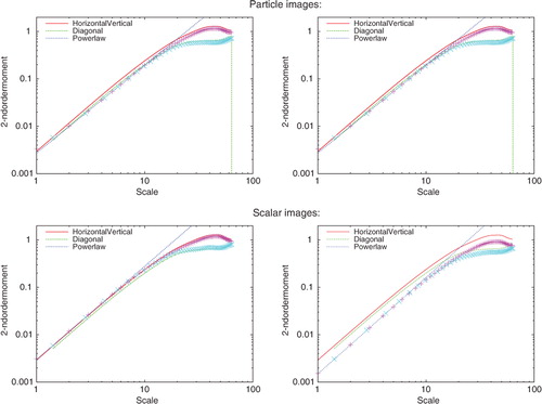
Figure 3 shows the shape of the evidence according to the power law model parameters. The model probability global maximum is located at the coordinates ζ=0.0030 and γ=1.975 (resp. б=0.00275, γ=1.850) for the particle (resp. scalar) images. Three observations assess experimentally the Bayesian criterion used for model inference. First, Fig. 3 shows that, specially for particle images, the parameters yielding high model probabilities correspond to low root mean square (RMS) motion reconstruction errors. Second, this correspondence is not so remarkable in the case of scalar images, because minimising an RMS error criterion does not always lead to the underlying power law. Indeed, as shown in the plots of Fig. 4, the inferred power law parameters are for both experiments very close to the values б=0.003, γ=1.948 obtained by an LS fit on the ground truth motion field, whereas on the contrary in the case of scalar images, choosing the power law minimising the RMS error induces a slight bias. Remarkably, the reconstructed structure functions S₂(ℓ) in x- and y-directions (horizontal and vertical in the images) as well as in the diagonal directions adjust well the structure functions computed directly from the simulation (indicated by the straight lines) in a wide range of scales, and well beyond the range used for the regularizer. Third, between 1 and 8 pixels, the power law of all structure functions is close to ∼ℓ², which is the expected value from the theory in the inertial or dissipative range. It is also observed that the simulation approaches isotropic statistics at small scales since structure functions calculated in horizontal–vertical and in diagonal directions are nearly identical.

Fig. 3.  Energy of probability and RMS error behaviour w.r.t. power law parameters. Plot of minus of the log of the power law model evidence probability (left) and the motion RMS error (right) w.r.t. power law exponent ζ (ordinate) and prefactor γ (absciss) for the particle (above) and scalar (below) image sequences. The coordinates of the minima are plotted with yellow squares. These coordinates have to be compared with the true power law parameters , given by an LS fit of the DNS data.

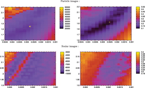
Fig. 4.  Second-order structure function reconstruction. Left plots: Inferred power law model represented by a blue dashed line, and estimated (resp. true) second-order structure function in horizontal-vertical directions plotted with stars (resp. continuous line) and in diagonal directions with cross (resp. dashed line). Right plots: identical legend for the motion estimate obtained with the prior power law model minimising the RMS error.

Therefore, maximising the model evidence constitutes a theoretically sound and reliable criterion for selecting the prior power law.

5.1.2. Evaluation of motion estimation.

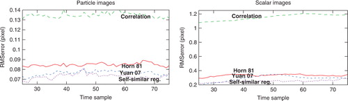
A comparison with state-of-the-art methods based on the RMS reconstruction error3 is provided in Fig. 5. Based on this criterion, the proposed method outperforms in average most accurate operational correlation-based techniques, first-order (Horn and Schunck, 1981) and div-curl (Corpetti et al., 2002; Yuan et al., 2007) regularizers.

Fig. 5.  Motion estimation accuracy. Evolution of RMS error w.r.t. time index for an operational correlation-based method, a robust first order regularizer (Horn and Schunck, 1981), a second-order regularizer (Yuan et al., 2007), and the inferred self-similar constraints for the particle (left) and scalar (right) image sequences. The results obtained with correlation approach were provided by LaVision (www.lavision.de) company from their operational PIV software (Davis) in the context of the Fluid FET Open European project.

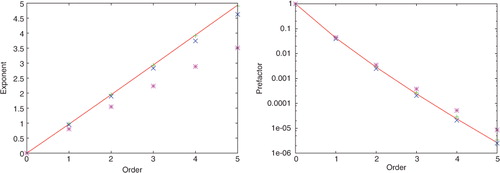
To assess quantitatively the accuracy of the reconstruction of the velocity increment PDFs, we plotted in Fig. 6 the exponents and the prefactors of structure functions w.r.t. their order. The exponents correspond to the dissipative range as they were computed by LS fitting of the reconstructed motion fields for increments of the structure functions between 1 and 8 pixels. Analysing the DNS motion field, it can be noticed that, in this range, the field is smooth and the exponents are on a straight line, as the structure function of order p, S _p (ℓ), goes as ∼ℓ ^p . The other estimates introduce spurious deviations from the straight line that may be incorrectly interpreted as intermittency. It is striking that the proposed method provides a very good estimation of the exponents and prefactors while all other methods fail to characterise exponents above the fifth order. This is a testimony of the power of the proposed motion estimation methods in recovering accurately the multi-scale structure of turbulence.

Fig. 6.  Longitudinal structure function exponents and prefactor w.r.t. their order for the scalar image sequence. The proposed self-similar regularization (crosses +) provides exponents (left plots) and prefactors (right plots) (in an LS sense) very close to the ground truth (solid line) in comparison to estimates of (Horn and Schunck, 1981) (stars *) or (Yuan et al., 2007) (× symbols). Correlation-based measurements are not presented here since they do not provide motion increments in the bottom of the scale range of [1, 8] pixels.

5.2. Atmospheric turbulence

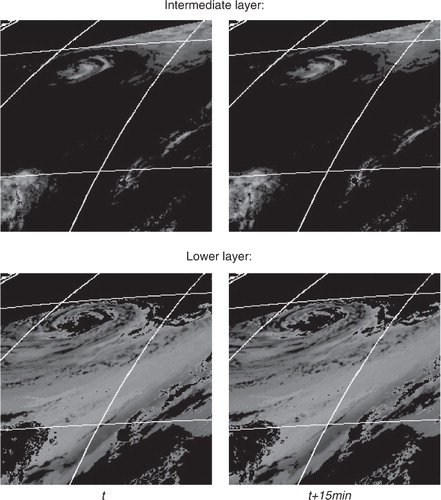
We now assess the inverse motion modelling approach using power laws on real data. The objective of this section is to estimate atmospheric parameters from satellite images, even when limitations associated to images and to required approximations may only give orders of magnitude of quantities of interest. We also compare results with previous observations using in situ techniques. The analysis is done using METEOSAT second-generation meteorological image sequences acquired above the North Atlantic Ocean at a rate of an image every 15 min during part of one day (5 June 2004), from 1200 to 1430 hour UTC (universal time, similar to GMT, the Greenwich Mean Time). Image spatial resolution is 3 × 3 km² at the centre of the whole Earth image disk. This benchmark data, which has been provided by the EUMETSAT consortium, is composed of images of top of cloud pressure and cloud-classification images. Cloud classifications were used to segment images into two broad layers, at low and intermediate altitude.4 Following the methodology described in Heas et al. (2007a) and in Corpetti et al. (2009), a set of sparse pressure difference images of 256×256 pixels associated to a stack of layers (low and intermediate altitude) was derived. Resulting set of input images is displayed in Fig. 7. As discussed before, an observation model is required for the inversion problem (see Section 2.1). An identical direct observation model as in Heas et al. (2007a) was used. It is based on layer mass conservation to relate image intensity function to vertically averaged horizontal wind fields.5

Fig. 7.  Depression over the north-Atlantic Ocean. Sequence of images depicting sparse pressure difference maps of layers at intermediate (above) and low (below) altitude. The images characterise the layers evolution in a time interval of 15 min and with an average spatial resolution of 3 km. Black regions correspond to missing observations and white lines represent meridians (20^o, 30^o and 40^o), parallels (50^o and 60^o) and the coastal contours of south of Greenland (upper left corner).

In the following, based on the work of Lindborg and Cho (2001), we first introduce prior knowledge on the sought power law using the Bayesian relation (27). The power law is chosen to model the longitudinal structure function of indifferently the zonal and meridional horizontal winds. Power law selection reduces then in this case to estimating the energy flux of the direct energy cascade toward small scales. We then relax this assumption and perform model selection considering a flat prior distribution on both unknowns: the power law prefactor and the power law exponent. Finally, we provide some statistical analysis and compare wind fields obtained with the two methods.

5.2.1. Power law selection with a Lindborg's prior.

In this section, we assume that the scaling б=2/3 predicted by Lindborg in the direct energy cascade holds in the range I=[1,4] pixels, equivalent to I=[3,12] km [the direct energy cascade is visible in the second-order structure function for separations of about 10 km in the data of Lindborg (1999)]. This hypothesis can be formulated in the Bayesian relation of (27) by choosing a prior such as , where δ and denote, respectively, the Dirac and the flat distributions. We thus only need to infer the parameter γ. Note that no power law is imposed for separations larger than 12 km.

5.2.1.1. Direct energy flux estimation

The model proposed in Lindborg (1999) provides power law models for the second-order structure function as:28

where b and c denote parameters and is a Kolmogorov constant. The energy flux ε (which is equal to the energy dissipation rate) can be related in the scale range I to the power law prefactor by . Therefore, maximising the power law posterior probability also reveals the most likely energy flux. Figure 8 shows that this probability is maximised for power laws with energy flux:29

Fig. 8.  Selection of most likely energy flux for Lindborg's model. Minus log of the power law posterior probability vs. energy flux ε in m² s⁻³ for horizontal winds at low (solid line) and at intermediate (dashed line) altitude.

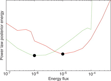
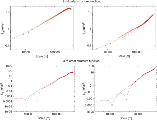
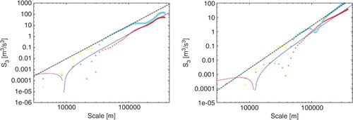
which correspond to estimates at low and intermediate altitudes. These estimates have the same order of magnitude as previously reported by results based on aircraft data analysis.6 The agreement is very good considering the measure is only based on image data. It should be noted that in the proposed estimation approach, as the evidence maximisation does not depend on motion variables, energy flux is obtained directly from the image intensity function, conversely to other approaches, which need to first extract motion observations from the images and then estimate power law parameters. One of the main results of the studies of Lindborg (1999) and Lindborg and Cho (2001) was to determine the direction of the energy cascade from the third-order structure function from in situ data. The third-order structure function can be reconstructed from the image-based motion measurements. Figure 9 shows this function for the lower and the intermediate layer. A direct cascade with linear dependence can be identified in the scale range [10, 40] km, and the agreement of the structure function for larger scales with the theoretical prediction seems reasonable.

Fig. 9.  Second- (above) and third-(below) order structure functions at low (left column) and intermediate (right column) altitudes. Second-order structure functions (+ symbols) are plotted with their associate models (dashed line). Third-order structure functions (plotted with × symbols for positive values and with + symbols for negative values) can be compared to their associate models (fine dashed line for positive values and coarse dashed line for negative values).

5.2.1.2. Direct enstrophy flux estimation

An LS estimate of the enstrophy flux can be obtained by fitting w.r.t. the third-order structure function to its model given by eq. (8) in the converged scale range (ℓ>50 km). In particular, at the upper range of the cascade, positive cubic power laws can be observed for both layers. The LS average enstrophy flux estimates are30 These results are also consistent with previously published results.7 Third-order structure function models obtained by LS estimation are displayed in Fig. 9. Second-order structure function and energy spectrum models given by eq. (28) can also be adjusted in an LS sense, and the parameters b and c can be estimated for scales l > 50 km. Figure 9 thus also shows the second-order structure functions and the energy spectra together with their corresponding models.

5.2.1.3. Moments convergence

To verify that we obtained converged statistics for the evaluation of the structure functions, we follow Gotoh et al. (2002) and examine the convergence toward a flat curve of the accumulated moments31 where is the PDF of the normalised increments with denoting the standard deviation. To check convergence of the second- and third-order structure functions, we examine the accumulated moments and see if there is convergence toward flat curves for increments associated to the tails of the PDF. Curves and show that the second- and third-order moments are reasonably converged. However, we observe that accumulated moments show a faster convergence for the lower layer motion. This obviously results from sparsity of image data, which increases with altitude. Furthermore, curves show that the third-order moments are better converged for large-scale increments (ℓ≳0 km) than for small-scale increments (ℓ≲0 km). This is in agreement with the fact that the normalised PDFs of velocity increments show stronger tails as the scale studied is decreased. These tails, which depart from Gaussian behaviour, are the result of intermittency: turbulence comes in gusts, and scarce regions with strong gradients develop in the flow as the result of non-linearities. The development of these strong events also makes the convergence of high-order moments slower, as more data are needed to have enough statistics to resolve the impulsive (but scarce) events. An extension of the present study to consider more images may enhance convergence.

5.2.2. Power law selection with a flat prior.

In this section, we now relax the previous scaling assumption and consider instead a uniform prior defined on the bi-dimensional parameter space (γ, б)∈ℝ² of the power law. Thus, we now also infer the most likely exponent of the power law together with the prefactor . Figure 10 shows that the selected prefactor (i.e., the energy flux) has the same order of magnitude as in the previous case. However, the selected power law exponent does not correspond to the model in (Lindborg and Cho, 2001). 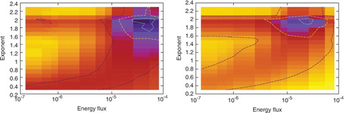Indeed, the second-order structure function maximising the evidence probability does not scale as but rather as ℓ² (at least, in the range of scales in which the constraint is applied; as will be shown next the structure functions scale in a similar way at scales larger independently of whether a scaling assumption or a uniform prior are used). Moreover, note that the model in (Lindborg and Cho, 2001) still corresponds to a region of high probability, i.e., a valley of the probability energy (marked by an iso-contour in Fig. 10). In the absence of ground truth, it is not obvious to decide whether one power law model is better than the other. One may conclude that using the images alone favours (in the particular case of these types of images) the choice of a low-complexity model that does not over-fit the data. In other words, the scaling of a regular motion is preferred, although more complex scaling is not drawn aside. When prior knowledge is available, the Bayesian modelling framework is able to enforce relevant regions of lower probability and recover accurately complex turbulence scaling laws.

Fig. 10.  Power law evidence probability. Minus log of model probability w.r.t. parameters: exponent ζ (ordinate) and energy flux ɛ in m² s⁻³ (absciss) (i.e., prefactor ), for horizontal winds at low (left) and at intermediate (right) altitude. Iso-contours of decreasing values around the minima are plotted in dark blue, yellow and turquoise.

5.2.3. Comparison of wind field estimates.

Deviation from strict self-similarity of the two motion estimates can be evaluated based on the behaviour w.r.t. their order of the structure function exponents (obtained by LS fitting of the reconstructed motion fields in the scale range of 1 to 6 pixels, corresponding to 3 to 18 km). Analysing the results in Fig. 11, it can be seen that we obtain a stronger deviation from linearity with the model of Lindborg and Cho (2001). However, in both cases the motion field is multi-fractal and not strictly self-similar.

Fig. 11.  Deviation from strict self-similarity at small scales (3–18 km) and at larger scales (30-80 km). Longitudinal structure functions exponents w.r.t. their order at low (solid curve) and intermediate (dashed curve) altitude using the model in (Lindborg and Cho, 2001) (on the left) or a flat prior (on the right) for power law models. The dashed straight lines represent strict self-similar behaviour, i.e., a linear relation of exponents w.r.t. order for the two models.

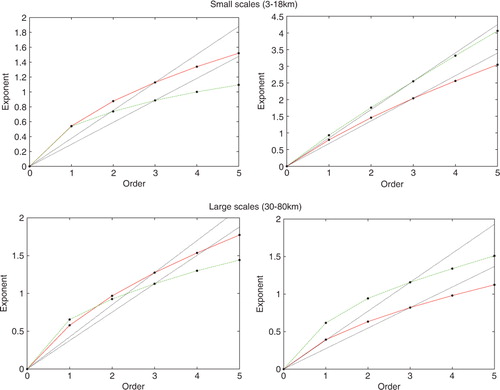
Exponents in Fig. 11 were computed for a similar range of scales as the one used for power law selection (3 to 12 km). It is thus not surprising that the second-order exponent changes substantially (as well as the other exponents), as in that range the method with the flat prior selected scaling ∼ℓ². This change in the exponents should be understood in the same light as the change in the reconstructed power law of the second-order structure function: images are favouring a model of lower complexity with regular motion at small scales.

However, structure functions show similar slopes and features for both reconstructions outside the range used for power law selection (e.g., for scales larger than 40 to 80 km depending on the altitude). It is not the motivation of our work to do a detailed analysis of scaling exponents at intermediate scales for atmospheric data, but just as an example, in Figs. 11 and 12 we show the third-order structure functions for low- and mid-altitude using both methods, and the scaling exponents at larger scales (10 to 30 pixels, or 30 to 90 km) for the model of Lindborg and Cho (2001) and for a flat prior. Two features are worth mentioning. In Fig. 12, note that not only amplitude of structure functions is similar in both cases (as already mentioned, as the amplitude of these functions is associated to the energy flux) but also that structure functions change sign at similar scales. In Fig. 11, exponents are similar at intermediate scales independently of the method used to reconstruct the field.

Fig. 12.  Third-order structure functions’ absolute value at low (left) and intermediate (right) altitudes for the two methods. Structure functions obtained with a (Lindborg and Cho, 2001) (resp. a flat) prior are plotted with×symbols (resp. □symbols) for positive values and with + symbols (resp. * symbols) for negative values. Estimate obtained with the (Lindborg and Cho, 2001) prior can be compared to their associate models (fine dashed curve for positive values and coarse dashed curve for negative values). At large scales, estimate obtained with both priors scale as ∼ℓ³ (straight dashed line).

Figure 13 compares motion fields obtained with our method (prior power law in ℓ²) with a vector field obtained by a correlation-based method. It is conspicuous that, for these very sparse and noisy images, correlation yields spurious and incoherent motion estimates while our approach yields a coherent and physically plausible reconstruction. Scaling in ℓ² tends to produce vortex and divergent structures of larger magnitude than for scaling in ℓ^2/3. Motion fields may present what could be interpreted as local abrupt discontinuities when visualised at larger scales. Indeed, the proposed optic-flow method provides a velocity vector per pixel. Therefore, small vortex and divergent structures of only a few pixels size may be confused with noise. In order to remove the confusion, we plot results at the pixel level. As shown in Figs. 14 and 15, velocity fields at this resolution appear to be very smooth and structured. In particular, vortex, sinks and sources are coherent structures of comparable order as claimed in Lindborg, 2007.

Fig. 13.  Estimated horizontal wind fields compared to correlation results. Dense wind fields at low (left) and intermediate (right) altitude where obtained using the flat prior, i.e., a scaling in ℓ². The correlation results were obtained using the operational PIV software (Davis) from LaVision (http:\\www.lavision.de) company.

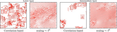
Fig. 14.  Detail of horizontal winds at low altitude. From top to bottom: input image (zoom between the 20^o and 30^o meridians and the 50^o and 60^o parallels), solenoidal (2 following lines) and divergent part (2 last lines) of motion estimated with a scaling of ℓ^2/3 (second and fourth line) or ℓ² (third and fifth line).

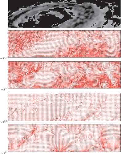
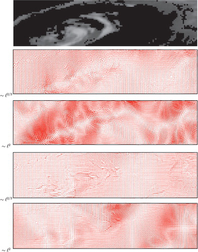
Fig. 15.  Detail of horizontal winds at intermediate altitude. From top to bottom: input image (zoom between the 20^o and 30^o meridians and the 50^o and 60^o parallels), solenoidal (2 following lines) and divergent part (2 last lines) of motion estimated with a scaling of ℓ^2/3 (second and fourth line) or ℓ² (third and fifth line).

6. Conclusions and perspectives

In this study, we presented a physically based, multi-scale method that does not involve any tuning of regularization parameters for fluid motion modelling from images. It relies on a Bayesian hierarchical model, which simultaneously provides optimal solutions for two problems: motion estimation and regularization model selection. The regularization models arise from Kolmogorov's work on turbulent flow self-similarity and recent results in the study of turbulent flows. Structure functions are used to exhibit some regularity in velocity field reconstruction, without a priori imposed power law. Besides achieving motion inversion, the method recovers several quantities of physical interest in turbulence. Moreover, for images of turbulent flows (or for laminar flows) where dissipative range is resolved, small scales are smooth and the proposed method reduces in fact to a smoothing with, e.g., null second-order structure function, or with the second-order structure function proportional to the square of the spatial increment. Experiments on a synthetic sequence show that the method is more accurate than the best fluid-dedicated motion estimators. As a result, we believe the method constitutes a valuable tool for physical characterisation of turbulence from images. In particular, we were able to recover consistent flux across scales in atmospheric turbulence at different altitudes from a meteorological image sequence. Results are also consistent with theoretical predictions and with previous studies using in situ measurements.

We believe that this work opens interesting perspectives for observational characterisation of turbulence. Characterisation of turbulence cascades could also be performed by analysing other meteorological (or laboratory) images, depicting for instance evolution of passive scalars, water vapour, or temperature fields. Of course, the method requires a proper direct image observation model for each problem of interest, and as a result may have to be complemented with other measurement techniques for validation. However, we believe that the results presented here are promising and give a useful tool to complement other measurements in the difficult problem of turbulence characterisation. Inferring directly the scale range on which the prior power law should be exhibited according to the observed images represent an interesting perspective which is in principle straightforward considering a Bayesian framework. It would present the advantage to extend the set of possible power law multi-scale models considered for selection to traditional single scale regularizers, which represent power law particular cases. Another interesting perspective could concern the addition of a prior dynamical model to ensure dynamical consistency along time. Several works relying on variational image assimilation techniques have recently been proposed in this direction (Papadakis and Memin, 2008; Corpetti et al., 2009).

Acknowledgements

The authors acknowledge the support of the French Agence Nationale de la Recherche (ANR), under grant MSDAG (ANR-08-SYSC-014) ‘Multi-scale Data Assimilation for Geophysics’.

Notes

¹Let us outline that in the case of large displacements, the brightness constancy model (1) is generally replaced by its time-integrated form I(x+v dt,t+dt)−I(x,t)=0 linearised around some initial solution x+vdt. For the sake of clarity we will not describe the time-integrated model further even if its application is in practice essential to recover long-range velocity fields (see Heitz et al. (2010) and references therein).

²The hypothesis of isotropy can be relaxed; see, e.g., Taylor et al. (2003). The method to recover isotropic statistics described there motivates the use of different directions for the displacements in Section 3.1.

³ To compute RMS error on the pixel grid, true velocity fields have been interpolated since they are given on a shifted (by half a pixel) grid by DNS.

⁴Stratus and stratocumulus (resp. altostratus, atltocumulus and nimbostratus) are classified in the lower layer (resp. the intermediate layer).

⁵Let us remark that one can not guarantee that the data model which has been proposed in Heas et al. (2007a) is valid for regions where the model assumptions are violated (e.g., for non-layered structures) or for too noisy input observations (e.g., due to cloud classification errors or pressure retrieval errors). However, the local weakness of the observation model is balanced in our approach by the introduction of the relevant prior information on turbulent motion regularity.

⁶A collection of other aircraft measurements (Nastrom et al., 1984) shows a typical value in the troposphere close to ∼3×10⁻⁶ m²s⁻³ (Lindborg, 1999). Nevertheless, note that analogously to stratospheric observations (Dewan, 1997; Nastrom and Eaton, 1997; Cho and Lindborg, 2001), one should consider a significant variability in measurements.

⁷These values agree well with an early estimate of ∼10⁻¹⁵ s⁻³ obtained in Charney (1971). Authors in Tung (2003) then re-obtained this same result from simulations. Note, however, that enstrophy flux is slightly lower than the estimated∼10⁻¹³ s⁻³ of Lindborg (1999) using Nastrom et al. (1984) aircraft data.

⁸ Note that the precise values on the boundaries need not be specified since they modify the content of vector b but do not have any impact on the Hessian matrix A. Indeed, the form of the matrix is slightly changed to code Dirichlet boundary conditions, but its content is independent of the boundary function.

Appendix A: Solution of the constrained motion estimation problem

In this appendix, we show how to solve optimally the constrained problem given by eq. (13).

A1. Problem discrete formulation

Let us first express this problem in its discrete form. The derivatives related to any quadratic data term w.r.t motion v (e.g., the model of (4)) can be expressed in the matricial form A ₀ v−b ₀, when discretized on an image grid S of m points. The two discretized components of v∈ℝⁿ now represent a field of n=2m variables supported by the grid S, A ₀ is n×n symmetric positive definite, and b₀ ∈ℝⁿ represents a vector of size n. The discrete data term can then be rewritten as:A1 where c₀∈ℝ denotes a scalar. The discretisation of the self-similar constraints defined in eq. (11) implies the discretisation of the second-order structure function defined in eq. (7). The integral over θ yields a sum on 8 directions: 4 horizontal–vertical directions and and 4 diagonal directions of the bi-dimensional plane. The continuous motion field discretisation yields to rewrite the integral over the spatial domain Ω with a sum over the pixel grid S . On this regular grid, the longitudinal velocity increment function is available at scale ℓ either for on horizontal n _h and vertical n _v directions, or for on diagonal directions . To avoid using boundary conditions, we exclude of the sum the grid points which belongs to image borders of width ℓ. A node subset is thus defined depending on scale. Therefore, at scale ℓ, the discrete second-order structure function reads :A2 where we have denoted the number of nodes of the grid S ^ℓ by . The quadratic constraint derivatives can be expressed in the vectorial form , where are symmetric positive semi-definite matrices and are vectors of size n. Indeed, manipulating the derivative of the expectation of eq. (A2) w.r.t. the motion field v, one obtains for grid points in the subset S ^ℓ a new expression for the sth component of the constraint derivatives A3 where represents a discrete Laplacian operator with a centred second-order finite difference scheme defined on a grid rotated of with mesh point spacing equal ℓ to and where , and are similar to the discretisation of second-order spatial derivatives in a centred second-order finite difference scheme on a mesh with spacing of ℓ. The constraints can finally be written in their discrete form as,A4 where .

Let us remark that the discretisation of the self-similar constraints does not rely on any approximation, conversely to standard regularization schemes such as in Horn and Schunck (1981) where continuous spatial derivatives have to be approached by discrete operators. The self-similar model introduced here consists thus in a multi-scale generalisation of the first-order regularizer where the smoothing parameters are in this case related to the power law and given by the Lagrange multipliers. The constraint motion estimation problem defined in eq. (13) can thus be rewritten in its discrete form as,A5

A2. Dual problem and optimal solution

We are now interested in defining optimality conditions taken into account the constraints. To this end, the Lagrangian function is introduced asA6 In the Lagrangian duality formalism, the optimal solutions of the so-called primal problem P are obtained by searching saddle points of the Lagrangian function. The saddle points, denoted by (v ^*, λ ^*), are defined as the solutions of the so-called dual problem D, withA7 where denotes the dual function. As the functions f _d and are convex and as the constrained group is not empty, for positive Lagrangian multipliers , L is convex and the minimisation problem (P) has a unique saddle point, i.e., an optimal solution v ^* which is unique. More details of convex functionals and the convergence of the related minimisation problems can be found in Weickert and Schnörr (2004). Lagrangian multipliers , which represent the regularization parameters at scales , are then optimally given by the coordinates of the saddle point. Note that for negative Lagrangian multipliers, the convexity of the functional is no longer insured, and there is no guarantee of the solution unicity. Nevertheless, there still exist local optimal solutions.

A3. Convex optimisation

We focus now in the strategy to obtain the saddle point solution of the constrained estimation problem. The minimum of a locally convex Lagrangian function at point can be obtained by cancelling the gradientA8 which reduces (using (A1) and (A4)) to solving the large linear systemA9 In Appendix A1, we showed that the linear system components are constituted by the superposition of a collection of discrete operators obtained in a centred second-order finite difference scheme on a grid of mesh ℓ, which corresponds to second-order derivatives at different scales. Since we have no guarantee that the matrix is positive-definite depending on the sign of Lagrangian multipliers , the solution of the large system given by eq. (A9) is efficiently achieved using a conjugate gradient squared (CGS) method with an incomplete LU pre-conditioner. The dual function is then given byA10 The dual function is by definition concave and possesses so-called sub-gradients equal to . We employ a classical gradient method to find which maximises the dual function and thus obtain the solution . Finally, the constrained motion estimation method results in an Uzawa algorithm, which is used to converge toward the saddle point , i.e., the optimal motion estimate under self-similar constraints. An important remark is that once the regularization coefficient vector has been estimated for two consecutive images of the sequence, assuming motion stationarity, only one step of the Uzawa algorithm is needed to process the following image pairs. Therefore, the complexity of the algorithm reduces to the resolution of the linear system by CGS, that is, , where is the conditioning number of . The Uzawa algorithm is briefly presented hereafter.

• Iterate until convergence from point

  • At iteration k, compute motion solution of eq. (A9).

  • Define by a gradient ascent step:

• At convergence:

where represents a vector whose components are and and denote the step size and a positive-definite matrix defined at iteration k. The latter parameter and matrix can be fixed at each iteration to formalise a quasi-Newton algorithm satisfying the strong Wolf conditions (Nocedal and Wright, 1999).

Appendix B: Maximum likelihood estimate of the observation model error variance

To obtain an analytical expression of the variance of the observation model error maximising the evidence, we first detail analytically the three different partition function composing the evidence, then give an analytical expression of its derivate w.r.t. β and, finally, provide an expression for the ML estimate cancelling out the evidence derivative.

B1. Evaluation of the evidence for β

First, the likelihood PDF energy related to a quadratic observation model is composed of the energy of a multi-dimensional Gaussian with m uncorrelated components of variance , where m is the number of point composing the image grid. Its partition function reads:B1 Therefore, we obtain:B2 Second, the partition function of the posterior PDF of (19) is an integral, which can be calculated using Laplace's approximation (see, e.g., MacKay, 2003):B3 where we recall that v ^* is the MAP estimate, and is the associated set of Lagrangian multipliers. Noting that the term vanishes since constraints are fulfilled, this yields:B4 where n=2m denotes the number of unknown velocity variables. For Gaussian distributions, the Laplace equality is exact and for other mono-modal distributions it still constitutes a good approximation (Gull, 1989). The determinant of such large and sparse matrices can be efficiently approximated via an incomplete LU decomposition.

Finally, the partition function of the self-similar prior of (18) does not exist since the PDF is degenerated and has an infinity set of maxima, corresponding to the infinite set of admissible velocity field solutions respecting the self-similar constraint. To make this prior well-defined, we use Dirichlet boundary conditions for evaluating the evidence. 8 Considering these boundary conditions, we get a Hessian matrix A which has a slightly changed form but which is full rank. As previously, the partition function can be calculated using Laplace's approximation:B5 As the set of admissible solutions for the self-similar constraint is not empty, the maximum value of the exponential term in (B5) is equal to 1, and one gets:B6 Replacing (B2), (B4), (B6) in (23), one obtains an analytical expression for minus the log evidence:B7 The evidence energy can be interpreted as the balance between three terms. The left term is the log likelihood. It represents the misfit of the data to the observation model. The two other terms appearing on the second line penalise the model complexity. They are known as the log of Occam's factor (Jaynes, 2003; MacKay, 2003). Of these, the first is the ratio of the posterior accessible volume on the prior accessible volume in v (a variance ratio in 1D). The term most to the right is a normalisation term of Occam's factor for non-unitary variance β.

B2. Derivative of the evidence and maximum likelihood estimate

To finally achieve the estimation of the observation model variance, we now want to minimise the energy of the evidence PDF. Noting that for any matrix C B8 one obtains the following equality:B9 Note that in the last expression (resp. ) does not (resp. does) depend on β. Using (B9), the derivative of log evidence (B7) w.r.t. β can be written as:B10 The log evidence is maximum at the point where the derivative cancels. Therefore, an analytical expression of the ML estimate of the observation model inverse variance reads:B11 Calculating the trace of the high-dimensional matrices involved in the previous equations can be very demanding. To overcome this problem, we use a trace randomisation technique (Skilling, 1989), which is efficiently achieved using the CGS algorithm. More precisely, random samples of an n-dimensional normalised and centred Gaussian distribution are used to approximate the trace operator:B12 where the vector is the solution provided by the CGS algorithm of the inverse problem , where is the unknown.

Appendix C: Likelihood probability of the prior power law

Since we have assumed that the prior p(β) is flat, the evidence is maximum at . Using Laplace's Gaussian approximation, the prior model evidence reads:C1 where the inverse variance is defined as a second-order derivative w.r.t. β of the evidence energy:C2 Using (B11), we obtain an approximation of the standard deviation at :C3 Finally, we obtain the energy of the evidence for model :C4 The prior model cancelling out the derivative of the previous energy can not be analytical obtained as it involves an inverse matrix operator. Therefore, to minimise the energy of the evidence for , the parameter vector is sampled uniformly in ℝ². The ML estimate is the minimiser of (C4) and represent the selected model.

Appendix D: Power law inference for laminar flows

Laminar flows are characterised by flat structure functions. Indeed, for such flows, increments are equal to zero. Therefore, power laws with vanishing prefactor constitute proper models for their structure functions. In the following we use a toy example in order to demonstrate the capacity of the proposed algorithm to recover accurately this particular case. Wu used a synthetic image (of 64×64 pixels) seeded with particles, which is evolved by a laminar flow (a translation by 1 pixel) to form the second image of the pair. Fig. 16 shows that the inference algorithm properly recovers the flat power law characterising such motions. It obviously corresponds to low RMS motion reconstruction errors as shown in the right part of the figure.

Fig. 16.  Power law evidence probability for laminar flows. True velocity field (left), plot of minus of the log of the power law model probability (centre) and the RMS motion reconstruction error (right) w.r.t. power law exponent ζ (ordinate) and prefactor γ (absciss). The line of minima which is selected by Bayesian inference corresponds to the true underlying power law (γ=0 for any ζ).

References

- Adrian R. Particle imaging techniques for experimental fluid mechanics. Annal. Rev. Fluid Mech. 1991; 23: 261–304.
- Baker, S.,Scharstein, D, Lewis, J. P, Roth, S, Black, M. J and Szeliski, R. 2007. A database and evaluation methodology for optical flow. Computer Vision, 2007. ICCV 2007. IEEE 11th International Conference on. , vol., no., pp.1-8, 14-21 Oct. 2007.
- Benzi R. Scardovelli R. Intermittency of two-dimensional decaying turbulence. Europhys. Lett. 1995; 29: 371–376.
- Bergen J. Burt P. Hingorani R. Peleg S. A 3-frame algorithm for estimating two-component image motion. IEEE Trans. Pattern Anal. Mach. Intell. 1992; 14(9): 886–895.
- Berliner M. Wikle C. Milliff R. Multiresolution wavelet analyses in hierarchical Bayesian turbulence models. Bayesian inference in wavelet based models. Lect. Notes Statis. 1999; 141: 341–349.
- Bernard D. Boffetta G. Celani A. Falkovich G. Conformal invariance in two-dimensional turbulence. Nature Physics. 2006; 2: 124–128.
- Boffetta G. Energy and enstrophy fluxes in the double cascade of two-dimensional turbulence. J. Fluid Mech. 2007; 589: 253–260.
- Carlier, J and Wieneke, B. 2005. Report 1 on production and diffusion of fluid mechanics images and data. Online at: Fluid project deliverable 1.2. http://www.fluid.irisa.fr.
- Charney J. Geostrophic turbulence. J. Atmos. Sci. 1971; 28: 1087–1095.
- Cho J. Lindborg E. Horizontal velocity structure functions in the upper troposphere and lower stratosphere 1. observations. J. Geophys. Res. 2001; 106: 223–232.
- Corpetti T. Heas P. Memin E. Papadakis N. Pressure image assimilation for atmospheric motion estimation. Tellus A: Dynamic Meteorology and Oceanography. 2009; 61: 160–178.
- Corpetti T. Mémin E. Pérez P. Dense estimation of fluid flows. Pattern Anal. Mach. Intel. 2002; 24(3): 365–380.
- Dewan E. Saturated-cascade similitude theory of gravity wave spectra. J. Geophys. Res. 1997; 102: 799–818.
- Falkovich G. Gawȩdzki K. Vergazzola M. Particles and fields in fluid turbulence. Rev. Mod. Phys. 2001; 73: 913–975.
- Fitzpatrick J. The existence of geometrical density-image transformations corresponding to object motion. Comput. Vision, Graphics, Image Proc. 1988; 44(2): 155–174.
- Frisch U. Turbulence: The Legacy of A.N. Kolmogorov. Cambridge, Cambridge University Press.1995
- Gotoh T. Fukayama D. Nakano T. Velocity field statistics in homogeneous steady turbulence using a high-resolution direct numerical simulation. Physics of Fluids. 2002; 14: 1065–1081.
- Gull, S. F. 1989. Developments in maximum-entropy data analysis. In Maximum Entropy and Bayesian Methods, J. Skilling (ed.). Kluwer Academic, Dordrecht. 53–71.
- Heas P. Memin E. Three-dimensional motion estimation of atmospheric layers from image sequences. IEEE trans. on Geo. and Rem. Sensing. 2008; 46(8): 2385–2396.
- Heas, P, Memin, E, Heitz, D and Mininni, P. 2009. Bayesian selection of scaling laws for motion modeling in images. In International Conference on Computer Vision (ICCV'09). Kyoto: Japan.
- Heas P. Memin E. Papadakis N. Szantai A. Layered estimation of atmospheric mesoscale dynamics from satellite imagery. IEEE trans. on Geo. and Rem. Sensing. 2007a; 45(12): 4087–4104.
- Heas P. Memin E. Papadakis N. Szantai A. Layered estimation of atmospheric mesoscale dynamics from satellite imagery. IEEE trans. on Geo. and Rem. Sensing. 2007b; 45(12): 4087–4104.
- Heitz, D, Carlier, J and Arroyo, G. 2007. Final Report on the Evaluation of the Tasks of the Workpackage 2. Technical report, Deliverable 5.4, Cemagref, Rennes, France.
- Heitz D. Memin E. Schnoerr C. Variational fluid flow measurements from image sequences: synopsis and perspectives. Exp. Fluids. 2010; 48(3): 369–393.
- Hoar T. J. Milliff R. F. Nychka D. Wikle C. K. Berliner L. M. Winds from a Bayesian hierarchical model: computation for atmosphere-ocean research. J. Comp. and Graph. Statis. 2003; 12(4): 781–807.
- Horn B. Schunck B. Determining optical flow. Artificial Intelligence. 1981; 17: 185–203.
- Jaynes E. T. Probability Theory: The Logic of Science. Cambridge, Cambridge University Press.2003
- Kolmogorov A. The local structure of turbulence in inompressible viscous fluid for very large Reynolds number. Dolk. Akad. Nauk SSSR. 1941; 30: 301–305.
- Kraichnan R. Inertial ranges in two-dimensional turbulence. Phys. Fluids. 1967; 10: 1417–1423.
- Kurien S. L'vov V. S. Procaccia I. Sreenivasan K. R. The scaling structure of the velocity statistics in atmospheric boundary layer. Phys. Rev. E (Statistical Physics, Plasmas, Fluids, and Related Interdisciplinary Topics). 2000; 61(1): 407–421.
- Leese J. Novack C. Clark B. An automated technique for obtained cloud motion from geosynchronous satellite data using cross correlation. J. Appl. Met. 1971; 10: 118–132.
- Lindborg E. Can the atmospheric kinetic energy spectrum be explained by two-dimensional turbulence. J. Fluid Mech. 1999; 388: 259–288.
- Lindborg E. Horizontal wavenumber spectra of vertical vorticity and horizontal divergence in the upper troposphere and lower stratosphere. J. Atmos. Sci. 2007; 64(3): 1017–1025.
- Lindborg E. Cho J. Horizontal velocity structure functions in the upper troposphere and lower stratosphere 2 theoretical considerations. J. Geophys. Res. 2001; 106: 233–241.
- Liu T. Shen L. Fluid flow and optical flow. J. Fluid Mech. 2008; 614: 253–291.
- Lucas, B. D and Kanade, T. 1981An iterative image registration technique with an application to stereo vision. In Proceedings of the 7th international joint conference on Artificial intelligence – Volume 2 (IJCAI'81), Vol. 2. Morgan Kaufmann Publishers Inc., San Francisco, CA, USA . 674–679.
- MacKay D. J. C. Bayesian interpolation. Neural Computation. 1992; 4(3): 415–447.
- MacKay D. J. C. Information Theory, Inference, and Learning Algorithms. Cambridge, Cambridge University Press.2003
- Monin A. S. Yaglom A. M. Statistical Fluid Mechanics: Mechanics of Turbulence. New York, MIT Press.1975
- Nastrom G. Jasperson W. Gage K. Kinetic energy spectrum of large and mesoscale atmospheric processes. Nature. 1984; 310: 36–38.
- Nastrom G. D. Eaton F. D. Turbulence eddy dissipation rates from radar observations at 5-20 km at White Sands Missile Range, New Mexico. J. Geophys. res. 1997; 102: 19495–19506.
- Nocedal J. Wright S. J. Numerical Optimization. Springer Series in Operations Research, Springer-Verlag, New York, NY.1999
- Papadakis N. Memin E. Variational assimilation of fluid motion from image sequences. SIAM J. Imaging Sci. 2008; 1(4): 343–363.
- Pedlosky P. Geophysical Fluid Dynamics. Springer, New York.1987
- Robert C. P. The Bayesian Choice: From Decision-Theoretic Foundations to Computational Implementation. Springer.2007; 577.
- Skilling, J. 1989. The eigenvalues of mega-dimensional matrices. Maximum Entropy and Bayesian Methods. Cambridge, England. 455–466.
- Taylor M. A. Kurien S. Eyink G. L. Recovering isotropic statistics in turbulence simulations: The kolmogorov 4/5th-law. Phys. rev. E. 2003; 2: 026310.
- Tung K. K. The k 3 and k 5/3 energy spectrum of the atmospheric turbulence: quasi-geostrophic two level model simulation. J. Atmos. Sci. 2003; 60: 824–835.
- Weickert, J and Schnörr, C. 2004. A theoretical framework for convex regularizers in pde-based computation of image motion. Int. J. Comp. Vis. 45(3). 245–264.
- Wikle C. K. Milliff R. F. Nychka D. Berliner L. M. Spatio-temporal hierarchical Bayesian modeling: tropical ocean surface winds. J. Amer. Statis. Assoc. 2001; 96: 382–397.
- Yuan J. Schnoerr C. Memin E. Discrete orthogonal decomposition and variational fluid flow estimation. J. Math. Imaging & Vision. 2007; 28: 67–80.