Multi-scale variability of winds in the complex topography of southwestern Norway

ABSTRACt

Multi-scale variability of winds in the complex terrain of southwestern Norway is investigated using up to 20 yr of observations from nine automatic weather stations and reanalysis data. Significant differences between the large- and local-scale winds are found. These differences are mainly governed by the large-scale topography of Southern Norway. Winds from the southeast and statically stable flow from the northwest are found to be significantly reduced at the ground level due to large-scale wake and blocking effects. Southwesterly and northeasterly winds are orographically enhanced. At a local scale, there are differences in the wind speed distributions between the surface stations, both in space and time. These differences can to a large extent be quantified in terms of the Weibull distribution function and associated with the respective geographical locations as discretised in four characteristic surface categories: offshore, inland, coast and mountain. The inland category is found to be associated with relatively low but variable wind speeds, whereas the coastal and offshore locations are dominated by more steady and stronger winds. The mountain wind speed distribution is fundamentally different from the others; it shares the variability with the inland locations but the higher average wind speed with the other categories.

• complex terrain
• Southern Norway
• flow modification
• topography
• local meteorology

1. Introduction

Along the southwest coast of Norway, southerly winds prevail throughout the year. On a timescale of days and weeks, however, the frequent passages of cyclones give rise to rapid and large changes, both in wind direction and wind speed. Of similarly great magnitude are the spatial differences found in smaller scale winds for a given large-scale flow. These differences are in first order governed by the larger scale topography of Southern Norway (approximately 100–150 km wide, 1500 m high), inducing phenomena that can be characterised as meso to synoptic-scale flow structures. At a local scale (1–50 km), the flow is modified by topographic features typical for the Norwegian coast such as steep mountains, valleys, narrow fjords, islands and straits. Also, contributing to the local-scale variability in winds are thermally driven flows such as land–sea breezes or valley and mountain winds. Meso to synoptic-scale flows over Southern Norway have been studied since the early days of the Bergen School of Meteorology (Bjerknes and Solberg, 1921, 1922). With an increased observational record, their findings later led to forecasting rules for different flow regimes. The findings were documented by Spinnangr (1943). Later, Andersen (1975) gave an overview of different wind patterns classified by periods of certain prevailing large-scale wind directions. In recent years, two papers have been published on the topic, Barstad and Grønås (2005), hereafter BG05) and Barstad and Grønås (2006). Using a series of idealised numerical simulations and reanalysis data along with ground observations, they studied flows over Southern Norway in the sector from south to west with emphasis on mesoscale flow structures. Among their main findings, was a jet forming along the mountain slopes and out over the sea (referred to as a ‘left-side’ jet) connected to southwesterly large-scale flow. In addition, lee side effects such as downslope-accelerated winds and a wind shadow connected to inertio-gravity waves were identified in southeasterly to southerly flow.

Under conditions with weak synoptic flow, thermally driven flows (flows driven by local temperature and pressure gradients) such as sea and land breezes, valley and mountain winds typically dominate on a local scale. In southwestern Norway, such local flow has mainly been studied in the Bergen valley and its surroundings. Berge and Hassel (1984) studied temperature inversions and local drainage flow in the Bergen valley using a tethered balloon and automatic weather stations (AWSs). They found the development of inversions to be most frequent in wintertime during periods with larger scale easterly (offshore) winds and high atmospheric stability. Utaaker (1995) studied the climate in Bergen, with the main emphasis on local winds and temperature conditions. He described a prominent channelling effect by the Bergen valley and a variation in dominating local wind directions with the time of the year, driven under weak synoptic flow to a large extent by sea breeze during summertime and katabatic winds during wintertime. An AWS at Flesland, some 10 km southwest of the centre of Bergen, was found to give the most representative picture of the wind field in the Bergen area as a whole.

In many ways, the southwest coast of Norway represents a physical barrier to the large-scale flow. In the aforementioned studies on such flow over southwestern Norway, this roughly north/south-oriented barrier has mainly been treated as a two phased one, with sea to the west and land/mountains to the east. Accordingly, this simplification has predominantly been used when describing flow regimes over the area (with one over land and one over sea). In this study, a more refined topography transition between sea and land is used, laterally dividing the coastal zone into four discrete surface categories: offshore, coastal, inland and mountain. By this new concept, the present study lays more emphasis on finer scales, allowing for a more detailed description of the flow over the southwest coast of Norway.

It is a main aim of this study to investigate the relationship between the large-scale flow, the aforementioned mesoscale flow structures and the flow at local scale. Previous studies on the relationship between the small- and large-scale flow in complex terrain, (e.g. Whiteman and Doran, 1993; Kalthoff et al., 2003) have found significant differences between the two but have not explicitly included mesoscale flow structures as those studied here. The present investigation is confined to a relatively limited area roughly covering the western/seaward half of the Hordaland county, centrally situated at the southwest coast of Norway (Fig. 1). The area is further on referred to as the ‘Greater Bergen area’. The results will, amongst other things, provide a climatological frame for an ongoing project, where a very dense network of AWSs is being established in the central areas of Bergen. In addition, the results will be of general relevance for local-scale weather forecasting in the area and may give guidance for estimations of, for example dispersion of pollutants.

Fig. 1.  Topography of Southern Norway with the area of main interest and the locations of the nine automatic weather stations. Gullfaks C is located some 80 km to the west of the indicated position. ‘ECMWF’ indicates the position from which the ECWMF reanalysis data are obtained.

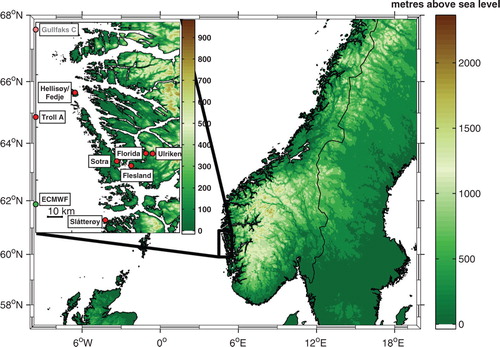
Up to 20 yr (1989–2009) of data from nine AWSs situated in a rough transect from offshore via the coast to the inland and the mountains are used. ERA Interim data from the European Centre for Medium-Range Weather Forecasts (ECMWF) are used to estimate the corresponding large-scale flow.

The second section of this paper is dedicated to a description of the data and theory.

Section 3 describes the results, section 4 presents a discussion of these and the main findings are summarised in the fifth and last section.

2. Data and theory

2.1. Atmospheric data

In the area of interest, i.e. the Greater Bergen area as defined in the introduction, a number of AWSs have been erected to provide information on the local climate. The AWS at Mount Ulriken is run in a collaboration between Aanderaa data instruments (AADI) and the Geophysical institute, University of Bergen (GFI), and the AWS at Sotra is run by Avinor. The remaining stations are operated by the Norwegian meteorological office (met.no). The geographical locations of the AWSs are indicated in Fig. 1, and key figures for each station are listed in Table 1. At Florida, the measurements are made on the top of the GFI building around 25 m above the surrounding ground. The wind speed there is, therefore, most likely somewhat higher than the typical 10 m reference value. The measurements offshore, i.e. at the platforms of Troll A and Gullfaks C, are also made at higher altitudes (approximately 70 and 77 m.a.s.l.).

Table 1. Automatic weather stations

Station	Dates	Source	m.a.s.l.
Florida	1989–2009	met.no	48
Flesland	1989–2009	met.no	48
Ulriken	2005–2009	AADI/GFI	605
Sotra	2007–2010	Avinor	341
Hellisøy	1989–2005	met.no	20
Fedje	2004–2009	met.no	19
Slåtterøy	1989–2005	met.no	25
Troll A	1998–2009	met.no	Approximately 70
Gullfaks C	1990–2009	met.no	77
ERA Interim-850 hPa	1989–2009	ECMWF	N/A
ERA Interim-925 hPa	1989–2009	ECMWF	N/A
ERA Interim-10 m	1989–2009	ECMWF	N/A

For most of this study, the meteorological data are obtained as 10 minute averages every 6 hours, i.e. 0000, 0600, 1200 and 1800 UTC. Not all station data are available with a full 20 yr record. These inhomogeneities might have implications on the accuracy of, for example the calculations of the Weibull factors, as presented in Section 3, and more data in future records would be expected to yield more accurate estimations. The same holds for the wind ratios presented in the same section.

Following the concept given in the introduction, the AWSs are grouped into four categories according to their geographical locations, that is offshore, coast, inland and mountain. No regular upper air observations are made in the area; therefore, ECWMF ERA Interim 850 hPa reanalysis data (hereafter ‘ERA Interim’) from a point at 60°N 4.5°E are used to estimate the large-scale wind direction and wind speed. The ERA Interim data have a temporal resolution of 6 hours and a horizontal grid spacing of 1.5°.

2.2. Theory

2.2.1. Mountain flow.

Rotunno and Ferretti (2001) list the following five central parameters in the theory of orographic flow modification (neglecting the effects of latent heat release): The typical wind speed of the background flow, U, the Coriolis force f, the Brunt–Väisälä frequency N, the obstacle (mountain) height h and L, a length scale commonly considered as the mountain half-width in the direction of the flow. The effect of these parameters are nicely summarised in Fig. 11 of their paper. The five parameters are often combined to form three different non-dimensional control parameters (e.g. Birkhoff, 1960): The non-dimensional mountain height (or inverse Froude number) Nh/U, the Rossby number U/fL and the hydrostatic number U/NL.

For a linear, stratified flow over a mountain on a frictionless, non-rotating plane, the main parameter governing the flow is Nh/U (Pierrehumbert and Wyman, 1985). In the literature, various flow regimes based on this parameter are described (e.g. Peng et al., 1995; Triib and Davies, 1995; Lin and Wang, 1996; Ólafsson and Bougeault, 1996). Smith (1989) outlined three main flow regimes over simple 3-D mountains: Low values of Nh/U enable the flow to pass over the mountain without any stagnation, and typically gentle gravity waves are formed. Nh/U can be seen as a measure of the non-linearity in the flow, and linear theory describes the response well in this range (Gill, 1982). For high values of Nh/U, the flow may stagnate on the upstream side of the mountain, and this is the most common pattern for high mountain ranges. On a non-rotating plane, for a mountain that is elongated along the flow, stagnation starts at values of Nh/U that are higher than if the mountain is elongated across the flow (Smith, 1989). This has been confirmed by Bauer et al. (2000), using 3-D numerical simulations. Neglecting the effects of rotation, westerly flow should in other words be more easily blocked than southerly flow, both impinging on a mountain with the shape of Southern Norway (north–south elongated).

The Rossby number enters the theory as an additional parameter for flow on a rotating plane. As the flow impinges on the mountain, it is decelerated by the buildup of a pressure surplus on the upstream side created below the air that is cooled off through adiabatic ascent as it is forced to climb the mountain. The deceleration causes a net force imbalance in the initially geostrophic flow leading more of the flow towards the left of the mountain (in the northern hemisphere). This effect is well described in the literature (e.g. Smith, 1982; Pierrehumbert and Wyman, 1985). Rotation, thereby, may render flow that would be blocked on a rotating plane, unblocked (Thorsteinsson and Sigurdsson, 1996; Ólafsson and Bougeault, 1997). The effect of the mountain aspect ratio on a rotating plane is the opposite of that for a non-rotating plane. For Southern Norway, it facilitates the westerly flow but not the southerly flow to overcome the blocking (Petersen et al., 2005). Finally, smaller scale topography impacts the flow on scales, where the Coriolis force is negligible and at these scales the flow may be blocked locally.

The intensity of upstream blocking critically depends on the ambient static stability that can modulate the magnitude and direction of the low-level flow impinging on the orography (e.g. Smith, 1979; Smolarkiewicz and Rotunno, 1989 1990). For strong atmospheric stratifications and through the above-described effect of rotation, left-bound barrier jets often form in connection to larger mountain ranges. They may be associated with cold air damming effects, as investigated by, for example Bell and Bosart (1998) for flow near the Appalaches and flow with high Nh/U as discussed by Pierrehumbert and Wyman (1985) and Overland and Bond (1993). Such jets are typically found along larger mountain ranges as the Rocky Mountains (Colle and Mass, 1995), the Appalaches (Bell and Bosart, 1998) and along mountainous coastal regions as those of Southern Norway (BG05), California (Doyle, 1997), Alaska (Overland and Bond, 1993) and Greenland (Ólafsson and Ágústsson, 2009; Renfrew et al., 2009). The terrain is the forcing element of the flow, so such jets are normally confined below the mountain peaks (Parish, 1982, BG05).

For Southern Norway, L varies between 100 km (westerly flow) and 250 km (southerly flow). This corresponds to a length scale found within the meso range. Typical wind speeds in the region are in the range 5–20 m s⁻¹, and the characteristic mountain height is around 1500 m. This would yield a typical Rossby radius from 0.15 to 0.65 for southerly/northerly winds and from 0.4 to 1.65 for westerly/easterly winds (BG05). These values are in the so-called intermediate range (e.g. Triib and Davies, 1995), where perturbations take the form of inertia buoyancy waves for R ₀ slightly above 1 and pseudo-geostrophic waves for R ₀ slightly below 1 (Pierrehumbert and Wyman, 1985).

2.2.2. Wind speed distribution.

Wind speed distributions have successfully been approximated by the Weibull probability density function (e.g. Justus and Mikhail, 1976; Hennessey, 1977; Pavia and O'Brien, 1986; Wei, 2010). The function can be expressed as follows:

f(x) gives the probability that a random observation has a value equal to x. k > 0 is the shape parameter and λ > 0, the scale parameter. k is dimensionless and λ has the units m s⁻¹. In short, the shape parameter k is a measure of the variability in wind speed.

The wind speed distribution in areas with high diurnal variability, for example, areas often experiencing local thermally driven flow, will typically be associated with a low shape parameter (k-values below approximately 1.8). The same is generally valid for regions with complex terrain. A low shape parameter k also indicates a high prevalence of low wind speeds. Regions with a more stable wind climate, such as the trade wind belt, are generally characterised by a higher shape parameter (k-values around 3). The scale parameter λ is tightly linked to the average wind speed. A high scale parameter indicates a high average wind speed and vice versa.

The cumulative Weibull distribution function, giving the probability that a random observation has a value equal to or less than an assigned value x, can be expressed as follows:

In this study, the scale and shape parameters are obtained through a maximum likelihood estimate. The calculations are based on 6 hourly data from the periods indicated in Table 1.

3. Results

3.1. Large-scale wind climatology

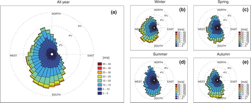
Looking at the wind distribution at 850 hPa derived from 20 yr of ERA Interim data (Fig. 2, a–e), it is clear that winds from the southeast through the westerly sector to the north are dominating. Winds from the east and northeast, on the other hand, are rare throughout the year. The highest wind speeds are generally found in the sector south to southeast. A seasonal variation is seen in both the wind direction and the wind speed. In the winter, the winds are more westerly than in the other seasons. The winter also has the highest wind speeds. The weakest winds are, as expected, found in summertime. Furthermore, the summer season is associated with dominating large-scale winds from the south and a higher portion of northwesterly winds than the rest of the year.

Fig. 2.  Climatology of large-scale winds (ERA Interim 850 hPa at 60°N 4.5°E) for (a) all year, (b) the winter (December–January–February), (c) the spring (March–April–May), (d) the summer (January–July–August) and (e) the autumn (September–October–November).

3.2. Frequency of wind directions

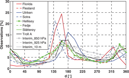
Figure 3 shows the relative frequency of occurrence of different wind directions at the selected AWSs. It appears that the most common wind direction at the ground level in the area is south-southeast. Similar to the flow at 850 hPa, winds at the ground level from east and northeast are rare. Although somewhat more frequent offshore (observations of wind direction at Gullfaks C are missing) and aloft, westerly winds are also generally rare. Close to 25% of the strong winds at Florida are south-southeasterly (150–170°), making it the single most common wind direction at any of the included locations. Undoubtedly, this is caused by a channelling through the Bergen valley. The second most dominating wind direction in the area is northerly (around 340°).

Fig. 3.  Distribution of wind direction, d (°), at the chosen surface stations and ERA Interim data in Table 1 for all local wind speeds. Wind direction data from Gullfaks C are missing.

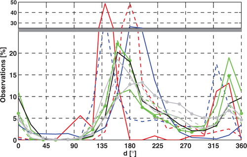
When excluding data corresponding to local wind (winds observed at each station) speeds below 10 m s⁻¹ (Fig. 4), one can see where the stronger winds come from. The south-southeasterly peak in wind direction distribution at Florida becomes even more pronounced, now accounting for close to 50% of the observations (although this is a rare event, see Fig. 6). The same effect is seen at Flesland. Also, the majority of the other stations report a significantly higher portion of wind speeds from the south for this higher wind speed threshold. A significant increase in relative frequency is also seen for northerly winds at most stations. Together with the increase in frequency of southerly winds, this indicates a stronger alignment to the coastline and general topography in the area for strong winds. Winds from the east and northeast of this magnitude are almost absent at all stations, with one notable exception, around 5% of the winds at Florida are easterly (100°).

Fig. 4.  Same as in Fig. 3 but for local wind speeds above 10 m s^–1. The thick, horizontal line at 25% corresponds to a change of scale in the y-axis. The change in scale is done to make the results below the line directly comparable to the results in Fig. 3.

3.3. Frequency of wind speeds

From the fitted Weibull distribution of wind speeds for the chosen AWSs (Fig. 5), a relatively close resemblance is found within each of the four location categories in Table 2. In terms of the Weibull shape parameter (k) and scale parameter (λ), as listed in Table 2, the inland locations are associated with a comparably low λ value (around 4) and a k ranging between 1.56 (Flesland) and 1.74 (Florida). The coastal and offshore stations, on the other hand, have larger λ values ranging from 7.29 (Slåtterøy) to 9.31 (Gullfaks C), or roughly twice that of the inland stations, and so are their mean and median wind speeds (7–8 m s^–1, not shown). These stations’ k values are also higher, around 2. The k and λ values for the stations at Mount Ulriken and Sotra appear as a combination of those from the three other categories: The k values are relatively low, similar to those at the inland stations, whereas the λ values are high, more similar to those found offshore and at the coast. In the case of Ulriken, the lower shape parameter corresponds to a higher frequency of wind speeds below 2 m s⁻¹, lower frequency of wind speeds between 2 and 15 m s⁻¹ and a higher frequency of wind speeds exceeding 15 m s⁻¹ when compared to the observations offshore and at the coast.

Fig. 5.  Fitted Weibull distributions of wind speeds, f (m s^–1), for the chosen surface stations and the ERA Interim data. The inserted panel (upper right corner) shows the upper tails of the distributions (wind speeds above 20 m s^–1) in more detail.

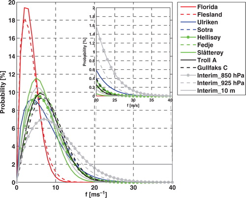
Table 2. Weibull shape and scale factors for the wind speed distribution at each station. The factor estimations are based on 6 hourly data from the respective data periods stated in Table 1

Station name	Location category	scale, λ [m s^−1]	Shape, k
Florida	Inland	3.99	1.74
Flesland	Inland	4.13	1.56
Ulriken	Mountain	8.03	1.48
Sotra	Mountain	8.4	1.81
Hellisøy	Coast	8.98	1.93
Fedje	Coast	8.79	2.08
Slåtterøy	Coast	7.29	1.94
Troll A	Offshore	8.68	2.00
Gullfaks C	Offshore	9.31	2.07
ERA Interim-850 hPa	Model	11.36	1.77
ERA Interim-925 hPa	Model	9.79	1.73
ERA Interim-10 m	Model	7.91	1.92

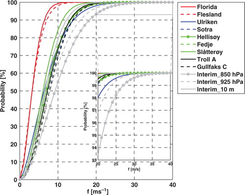
According to the cumulative Weibull distribution of winds (Fig. 6), showing the probability of having a wind speed equal to or less than a certain threshold (x-axis), only about 1% of the winds at the inland location of Florida exceed 10 m s⁻¹. This is significantly lower than that for, for example, Hellisøy/Fedje that is freely exposed to the North Sea, with a corresponding number of around 30%. At Mount Ulriken, around 25% of the winds are above 10 m s⁻¹ and 2% above 20 m s⁻¹.

Fig. 6.  Fitted cumulative Weibull distributions of wind speeds, f (m s^–1), for the chosen surface stations and the ERA Interim data. The inserted panel (at the right) shows the cumulative distributions for wind speeds above 20 m s^–1 in detail.

3.4. Seasonal and diurnal variations in wind speed

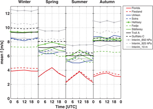
Figure 7 shows that the highest wind speeds are found during wintertime and the lowest during summertime. The overall strongest diurnal variations in wind speed are seen at the inland stations during summertime. In that season, the lowest wind speeds occur during night-time, whereas the highest ones are found around midday. A somewhat weaker diurnal variability in wind speeds is seen for the coastal stations. At the stations offshore, there is hardly any diurnal variability at any time of the year.

Fig. 7.  Seasonal and diurnal variation in wind speed, f (m s^–1), for the chosen surface stations and the ERA Interim data.

3.5. Surface winds and the large-scale flow

A question of central interest is how the local wind speed at the ground level varies with the large-scale flow. From the theory on mountain flow, as described in Section 2.2, this relationship is expected to mainly depend on the large-scale wind speed and wind direction and the atmospheric stability.

As a step towards answering the posed question, a wind ratio is introduced, defined as the median of the ratio between the local and larger scale wind speed:1

Situations with 850 hPa wind speeds below 5 m s⁻¹ and or with less than 20 cases are excluded from the calculations. Wind ratios are also calculated for model data at 925 hPa and 10 m above ground. The sensitivities of the wind ratio to the Nh/U, N and U have similarly been investigated by calculating the wind ratios for two different intervals of each parameter. The intervals are divided by high and low values of each parameter, and the differences in wind ratios between them correspond to the sensitivity.

In the calculations, h is set to the characteristic mountain height of Southern Norway, 1500 m. U is the average of the ERA Interim 850 hPa and 10 m wind speed and N, the Brunt–Väisälä frequency, is defined as follows:

where g,θ and z are the acceleration of gravity, the potential temperature and the altitude. Δθ and Δz are the differences in θ and z between 850 hPa and the ground and θ _avg is the vertical average of θ below 850 hPa. The thickness of the atmospheric layer, Δz, is obtained from the hypsometric equation. A dry atmosphere is assumed in the calculations.

The two different intervals of Nh/U are defined as follows: equal to or higher Nh/U than for 75% of all data (Nh/U  ≥  2.4) and equal to or lower Nh/U than for 25% of all data (Nh/U  ≤  1.1). The intervals for U are 5–10 m s⁻¹ and 10–15 m s⁻¹. For N, the two intervals are equal to or higher N than for 75% of all data (N  ≥  0.012 s⁻¹) and equal to or lower N than for 25% of all data (N  ≤  0.008 s⁻¹). In the context of N, only situations with 850 hPa winds in the range 10–15 m s⁻¹ are considered. This range is chosen to minimise the influence from variations in the ambient wind speed on the results and contains approximately 25% of the 850 hPa winds.

Figure 8 shows the wind ratio calculated over large-scale wind direction sectors of 20°. The corresponding results for the sensitivity of the wind ratio to Nh/U, U and N are presented in Figs. 9 10 11 .

Fig. 8.  Wind ratios for the surface stations and ERA Interim data as a function of the 850 hPa wind direction, d (°) for wind speeds at 850 hPa greater than 5 m s^–1.

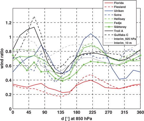
The wind ratios reveal two distinct wind regimes, one connected to strong surface flow and another to weak surface flow. These are discussed separately in Section 3.5.1.

3.5.1. Strong surface flow: Large-scale winds from southwest and northeast.

The, on average, highest wind ratios are found in connection to southwesterly flow. The response in the wind ratios to an increased Nh/U, as seen in Fig. 9 c, is on average higher wind ratios. Both U and N contribute to this increase as a decreased U (Fig. 10c) and an increased N (Fig. 11c) give higher wind ratios.

Fig. 9.  Wind ratios for cases with (a) low Nh/U and (b) high Nh/U and (c) the difference between both (a) and (b) (see the text for the definition of low and high Nh/U).

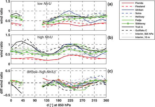
The second sector of relatively strong surface wind speeds is northeast. At the offshore stations, these maxima are, in fact, higher than in southwesterly flow. In contrast to, for example Flesland, Florida also observes relatively high wind speeds in this sector. Increasing Nh/U on average lowers the wind ratio for this wind sector (Fig. 9c) with contributions mainly from the static stability, N (Fig. 11c). The wind speed U works actively in the opposite direction (Fig. 10c). There are relatively few northeasterly cases, which is reflected by a large spread in wind ratios for this sector.

Fig. 10.  Wind ratios for cases with large-scale wind speeds from (a) 5 to 10 m s^–1 (b) 10 to 15 m s^–1 and (c) the difference between both (a) and (b).

3.5.2. Weak surface flow: large-scale winds from northwest and southeast.

In southeasterly large-scale flow, markedly reduced wind speeds are observed, not only at all surface stations but also at higher levels in the free atmosphere (ERA Interim 925 hPa data) (Fig. 8). The wind ratio appears on average quite insensitive to Nh/U and U for this wind sector.

Reduced wind speeds at the ground level are also found in large-scale flow from west and northwest. Increasing Nh/U gives, in general, lower wind ratios for this wind sector (Fig. 9c). The contributions are mainly from an increased N (Fig. 11c).

Fig. 11.  Wind ratios for cases with large-scale wind speeds from (a) 5 to 10 m s^–1 (b) 10 to 15 m s^–1 and (c) the difference between both (a) and (b).

3.5.3. Wind direction.

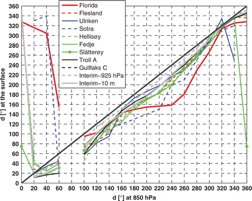
As expected from Ekman's theory, a general anti-clockwise shift in wind direction is seen at the ground locations when compared with the 850 hPa wind direction (Fig. 12). Deviations from the average shift of 20° are most notably found for large-scale wind directions from the west-southwest with an average shift in the order of 30–40° (anti-clockwise) and from north-northwest with no or even a negative (clockwise) shift of some few degrees. The station at Florida stands out as it observes winds from 130° and 160° in large-scale flow from south-southeast (160°) to west-southwest (240°). Similarly, for large-scale flow from north (0°) to northeast (40°), Florida observes winds from the northwest. These large deviations are caused by the channelling effect from the Bergen valley, as commented by Utaaker (1995).

Fig. 12.  Mean wind directions at the ground as a function of the 850 hPa wind direction.

3.6. Local-scale variations in the wind climate inland

Typically, the wind climate in complex terrain has a large variability, both in space and time. The central Bergen area is indeed dominated by complex terrain. At the location of Florida, the Bergen valley has an orientation of approximately 160/340° or south-southeast/north-northwest. The valley is rather open towards the sea in the northwest and somewhat more sheltered in the south. Ulriken, which is the highest mountain around Bergen (643 m.a.s.l.), is located 3 km to the east of Florida.

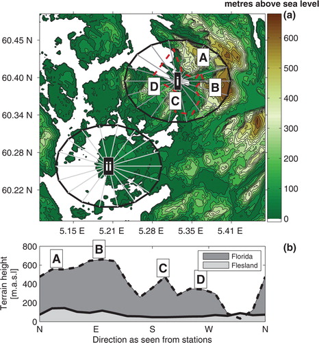
The local-scale wind variability in the Bergen area is here investigated using data from the stations at Florida and Flesland. Figure 13 shows a map over the central Bergen area together with profiles of maximum topography heights surrounding the two stations.

Fig. 13.  (a) Map over the central Bergen area with Florida in the northeast (i) and Flesland in the southwest (ii). The city centre of Bergen is marked by a red, dashed line. Both stations are shown with circles surrounding them with radii of 4 km. Each circle sector spans 20°. (b) The sectors’ maximum topography heights are plotted as a function of direction in relation to the respective stations. The topography curve for Florida is given labels from A to D indicating the geographical locations of the dominating topographic features around that location. Ulriken is marked by a ‘B’.

3.6.1. Wind speed.

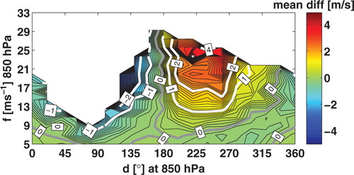
Figure 14 shows the mean difference in wind speed between the two stations (Flesland–Florida) with respect to the ERA Interim 850 hPa wind speed and wind direction. For large-scale wind speeds higher than 10 m s⁻¹ in the sector from south to west (170–290°), the mean wind speed at Flesland is consistently higher than at Florida. The maximum difference of around 4–5 m s⁻¹ is found for 850 hPa wind speeds in the range 21–27 m s⁻¹. For wind directions outside this sector, the wind speeds are either similar or higher at Florida than at Flesland, forming a dipole-like pattern with a positive difference for westerly winds and a negative difference for easterly winds.

Fig. 14.  Mean difference in wind speed between Florida and Flesland (Flesland–Florida) as a function of the 850 hPa wind speed, f (m s^–1), and wind direction, d (°).

3.6.2 Wind direction

Looking at Fig. 15 a showing the summertime diurnal variation in wind direction distribution at Florida and Flesland for all large-scale wind speeds, a clear bimodal pattern is seen at both locations. The daytime (approximately 0700–2200 UTC) is dominated by a northerly wind component, whereas the winds at night-time are more southerly. For large-scale winds below 10 m s⁻¹ (Fig. 15 b), an even larger portion of the winds at Florida is northwesterly. At Flesland, a similar daytime increase in the frequency of northerly winds is seen. Considering situations with large-scale winds above 10 m s⁻¹, as shown in Fig. 15 c, the wind direction distributions assume a character much more similar to that found during night-time, and only a slight diurnal signal is seen.

Fig. 15.  Diurnal variation in wind direction distribution at Florida (green) and Flesland (red) during the summer months June, July and August for (a) all 850 hPa wind speeds (f), (b) 850 hPa wind speeds below 10 m s⁻¹ and (c) 850 hPa wind speeds above 10 m s^–1. The statistics are based on hourly 10 minutes. Averages from the years 2005 to 2009.

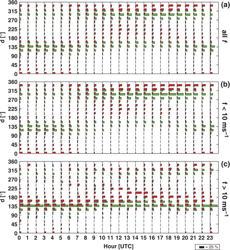
Differences between the two stations are mainly seen as deviations at Flesland from Florida's strictly south-southeast/ north-northwest-oriented wind components. These differences are especially evident during daytime, where Flesland has a larger prevalence of winds from the south and the west. Contributing to this difference is also a clockwise turn (veering) in wind direction with time at Flesland, which is not seen at Florida. The clockwise turn, as caused by the effect of Coriolis on the sea breeze circulation (e.g. Simpson, 1994), is presumably not evident at Florida because of the surrounding topography's tendency of aligning the wind along the Bergen valley's axis. It is clear that the sea breeze's presence depends on the magnitude of the large-scale wind speed. For wind speeds above 10 m s⁻¹, the daytime northerly wind components at ground are almost absent, whereas for large-scale wind speeds below 10 m s⁻¹, they dominate (Fig. 15).

Wintertime situations show, to a large extent, similar patterns as those found during night-time in the summer (not shown).

4. Discussion

In the present study, multiscale variability of winds in the complex terrain of southwestern Norway has been investigated using up to 20 yr of observational and reanalysis data. The wind field has been shown to have a large variability in both space and time over a relatively short distance from offshore, via the coast to the inland and mountain.

The content of this article can be summarised in three main themes: geographical differences in the local wind speed distributions, the relationship between the flow at larger and smaller scale and variations in the wind climate at the local scale. The following discussion is arranged accordingly.

4.1. Geographical variations in the wind speed distribution

It has been shown that the differences in wind character between four characteristic surface categories in the Greater Bergen area (mountain, inland, coast and offshore) can to a large extent be quantified in terms of the Weibull distribution function. The higher variability found inland, as reflected by the low Weibull shape factors (Table 2), may be explained by local circulations associated with the complex terrain such as features such as orographic blocking, wakes, gap winds and thermally driven flow. Sea breeze is, indeed, found to dominate locally inland during daytime in the summer as seen in Figs. 7 and 15 and as found by Utaaker (1995). The higher wind speeds found in the mountains, at the coast and offshore (as reflected by higher Weibull scale factors), as compared to inland, are presumably caused by the relatively lower surface roughness and the lack of sheltering from surrounding topography, both at scales below 5 km (Fig. 13) as well as at scales of Southern Norway (Fig. 16).

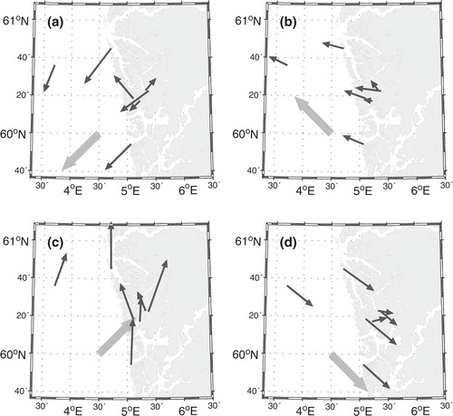
Fig. 16.  Mean wind direction and wind ratio at the surface stations (black arrows) as a function of four ERA Interim 850 hPa wind directions (thick, grey arrow): (a) northeast (35–55°), (b) southeast (125–145°), (c) southwest (215–235°) and (d) northwest (305–325°). The wind ratio is indicated by the arrow lengths. For a wind ratio of 1, the black arrow has a length equal to that of the thick, grey arrow, meaning that the wind speed is the same at the surface as at 850 hPa. All 850 hPa wind speeds are above 5 m s⁻¹.

The difference in Weibull scale factors between the coast and offshore locations is marginal. A distinct difference between these two categories, however, is the lack of diurnal variability in the wind speed offshore in summertime, but this difference alone has limited impact on the Weibull factors.

The current classification of surface categories through Weibull factors strictly only applies to the qualitative domain. A method, including a more statistical approach, to rigorously test to which category the stations belong could prove beneficial for future studies.

4.2. Variation in surface wind with the flow aloft

When considering the relationship between local and larger scale flow in the area, two main regimes stand out: relatively strong surface winds are found in southwesterly and northeasterly flow and weak surface winds are found for southeasterly flow (Fig. 8). Given a high atmospheric stability, relatively low surface wind speeds are also found in northwesterly flow.

BG05 also found strong surface winds along the southwestern coast of Norway in southwesterly flow. They attributed this flow nature to a coastal jet, mainly created by the effect of rotation deflecting the flow to the left, caused by a weakened Coriolis force as the flow is decelerated by the mountain. Petersen et al. (2005) described this kind of flow in their study of southwesterly flow impinging on an idealised mountain resembling the shape and north/south orientation of Southern Norway. A more than average deflection of the surface flow towards the left with respect to the flow aloft is indeed found for the southwesterly flow (Fig. 12). The surface wind speed is in this study shown to increase for higher values of Nh/U (Fig. 9) for the southwesterlies. This is in accordance with Overland and Bond's (1993) finding on the formation of jets along a mountainous coast line in Alaska as well as the idealised flow in Petersen et al. (2005).

In northeasterly flow, the surface wind is not far from being parallel to the height contours of the south Norwegian mountain range (Fig. 12). It is presumably accelerated by a pressure gradient associated with a wake at the west coast of South Norway.

Markedly reduced wind speeds are observed in southeasterly large-scale flow, not only at all surface stations but also at higher levels in the free atmosphere (ERA Interim 925 hPa data) (Fig. 8). This confirms the validity of the idealised numerical experiments made by BG05. They proposed an explanation in terms of a rather deep (more than 1500 m in some places), large-scale wind shadow forming downstream of the mountains in Southern Norway. They further suggested that this is not a classical wake, as typically occurring behind smaller scale mountains but a wake caused by rotational effects on the downstream inertio-gravity waves, as described by, for example Triib and Davies (1995). The wind ratio appears on average quite insensitive to Nh/U and U for this wind sector. There is no simple theory on how the mean surface wind speeds in wakes vary with U or Nh/U.

The surface winds in the northwesterly flow are quite variable in space and they are sensitive to the static stability, N. This indicates the presence of an orographic blocking with varying intensity and extension. Pierrehumbert and Wyman (1985) found through numerical simulations that the upstream horizontal extension of such blocking in a steep mountain zone is limited by the effect of rotation and is on the order of the Rossby radius of deformation, Nh/f. In the present case, for a value of N=0.01 s⁻¹, h=1500 m and f=10⁻⁴ s⁻¹, this would yield a deformation radius of 150 km. Even the most distant stations (Gullfaks C, ∼130 km and Troll A, ∼60 km) are within this distance from the mountains in Southern Norway. In the northwesterly flow, the weakening of the Coriolis force, as the flow impinges on the mountains, contributes to a leftward turning. This is towards the mountain range and thus supports the blocking. This is opposite to the Coriolis effect in the Southwesterly flow, where a turning to the left supports the left-side jet.

In summary, the effect of the atmospheric stratification, N, has an impact through two different processes. Firstly, it increases the Nh/U and thereby the magnitude of the oro-graphic disturbances, including the above-described left-side jet and the blocking. Secondly, it dampens the vertical mixing of momentum and reduces, thereby, the surface wind speed. In the southwesterly flow, the stability has, on average, no effect on the mean surface wind speed. The two processes appear, in other words, to compensate for each other. In the northwesterly flow, both processes contribute to a decrease in the surface wind as N increases: the blocking is increased and vertical mixing is decreased. This appears clearly in Fig. 11. In the southeasterly flows, the impact of N may contribute to increased surface winds through enhancement of gravity waves, but such effects are presumably quite local, and at our stations damping of the surface winds through less vertical mixing appears to be more important.

An effect left out in the above discussion is that of latent heat release. The release of latent heat has been shown to decrease the deceleration of flow impinging on a mountain and thereby facilitate for more of the flow to go over and less to go around the mountain (Rotunno and Ferretti, 2001; Miglietta and Buzzi, 2004). This effect would presumably be present in the target area, at least with flow from a sector of 90° around west, where most moist air masses originate. Thus, the release of latent heat may be a damping on both the northwesterly blocking and the coastal jet in the southwesterly flow. It is, however, unclear if this effect is important for the non-saturated surface flow that may be cooled by evaporation from precipitation at the same time. An increased N would also contribute to less vertical mixing of momentum and thereby lower the surface wind speed. Further investigations based on numerical simulations could shed some light on the importance of this effect in the area.

4.3. Variations in the wind climate at local scale

As an example of variations in the wind climate at local scale, the wind at Flesland, where the mountains are relatively far away, has been compared to the wind at the valley station at Florida. Both stations show markedly reduced wind speeds when compared to the flow aloft and the other investigated locations, but there are differences between them. The largest wind speed differences are found in southwesterly and easterly flow, averaging to about +4 m s⁻¹ and –2 m s⁻¹, respectively (Fig. 14). A possible explanation for the differences seen in easterly flow could be local downslope-accelerated winds, which have been found in easterly flow at inland stations in the area close to mountain slopes by Utaaker (1995). At Florida, these winds may be enhanced as they penetrate through the gap between two surrounding mountain ranges. Instances are found where these winds cause differences exceeding 12 m s⁻¹ (not shown). Such cases are, however, very rare.

The apparent sheltering of Florida in southwesterly flow (with respect to Flesland) can be related to its surrounding topography, as seen in Fig. 13. There are at least two likely explanations for these differences. One is the mountain massif to the southwest of Florida (marked ‘C’ and ‘D’ in Fig. 13), potentially creating a wake over the city centre of Bergen. Secondly, the mountain massif to the northeast (marked ‘A’ in Fig. 13) is likely to create a local blocking of the southwesterly flow. Whether this shelter effect is caused by a downstream wake, an upstream blocking or a combination of both is hard to assess using only the dataset at hand. Numerical simulations may answer this question. Interestingly, looking at Fig. 11 showing the effect of increasing the atmospheric stability on the wind speed at the ground, a markedly stronger increase in wind speed for an increased atmospheric stability is seen at Florida than at Flesland in southwesterly flow. The cause of this stronger wind speed increase at Florida could be related to a stronger channelling through the Bergen valley, forced by a higher Nh/U deflecting the flow around and channelling it in between the surrounding mountains. It may also be related to gravity wave activity aloft.

Sea breeze circulation induces a high diurnal variability in the local winds inland and at the coast in the summer months. This is seen as a 1200 UTC wind speed maximum (Fig. 7). At the mountain of Sotra, however, there is a maximum in the afternoon (1800 UTC). As at Florida, there is a clockwise turn in wind direction with time at Sotra during summertime and at 1800 UTC, the local wind is on average northwesterly (not shown). One possible explanation for this apparent shift in timing of the Sotra, the wind maximum is a local, orographic, wind enhancement for this wind direction. This would be consistent with the increase in wind ratio observed at Sotra for a shift from westerly (1200 UTC) to northwesterly wind (1800 UTC) (Fig. 8).

Interestingly, the diurnal variation in winds at Ulriken appears to be inverted when compared with the inland and coastal stations. The lowest wind speeds are observed during daytime and the highest during night, which is typically dominated by a relatively shallow, stable boundary layer. The peak of Ulriken, thereby, resides in a relatively undisturbed flow decoupled from the surface layer in the valley. During daytime, when the boundary layer grows higher than Ulriken, the wind speed at Ulriken is affected by the valley surface, and a downward-directed vertical mixing of momentum extracts energy from the mean wind. This argument is supported by the fact that the highest atmospheric stability, as estimated from the temperatures observed at Florida and Ulriken, is on average found during night-time (not shown).

5. Summary and conclusions

This article leads us to a series of conclusions of both general value as well as more specific value for the understanding of weather and climate of southwestern Norway and the Greater Bergen area.

While previous studies have focused mainly on either meso to synoptic- or small-scale phenomena (e.g. BG05 and Utaaker, 1995), this article has aimed at forming a link between the large-scale flow and processes at small scales. Central to this has been the verification of several mesoscale flow structures frequently forming over the area as numerically simulated by BG05, using several years of data from nine automatic weather stations along with ERA Interim reanalysis.

A new concept for describing the flow patterns along the Norwegian west coast has been introduced in the form of four characteristic surface categories: offshore, coast, inland and mountain. The concept has allowed for a detailed description of the flow in the investigated area and has furthermore been justified through a remarkable resemblance in wind character at the locations within each of the four categories.

The distributions of wind speeds in the area have been quantified in terms of the Weibull probability density function. The inland locations are found to be characterised by small scale and shape factors of, respectively, around 4 m s⁻¹ and 1.5, indicating generally low but highly variable wind speeds. The locations offshore and at the coast are associated with higher and more stable wind speeds, giving shape factors around 2 and scale factors around 8 m s⁻¹. The mountain wind distribution is fundamentally different and appears as a hybrid between the coastal/offshore and inland categories: It shares the shape factor with the inland and the scale factor with the coast and offshore locations.

Winds from the northeast and east are rare, not only at sea level but also in the mountains and at mountain top level in the free atmosphere (ERA Interim 925 and 850 hPa). The south and southwesterly winds are the most frequent aloft, which is in agreement with the position of the stormtrack.

The main findings on the relationship between the flow at larger scale and at the surface can be inferred from Fig. 16. In northwesterly large-scale flows, there is virtually no change in wind direction with height in the lower troposphere, whereas in southwesterly winds, there is strong clockwise turning (veering) of wind direction with height. This is clearly a topographic effect originating from the roughly south/north-oriented South-Norwegian mountain range and coastline, and the effect of rotation plays a central role. For large-scale flow from the southeast and statically stable flow from the northwest, surface winds are much weaker than the winds in the free atmosphere. This has been related to orographic blocking and wake. On the other hand, for large-scale flow from the southwest and northeast, the surface winds are relatively strong due to orographic enhancement.

Looking at the deceleration of winds at the surface, one would expect increased atmospheric stability to reduce the wind speed at the surface for any given wind speed in the free atmosphere due to damping of the turbulent vertical flux of horizontal momentum. This is, however, not the case in southwesterly flow, where the surface winds in stable flows on average are approximately the same as in unstable flows. However, in northwesterly flows, an unstable atmosphere gives relatively high wind speeds at the surface, and a stable atmosphere gives relative weak wind speeds at the surface. These findings have been related respectively to a left-side jet and orographic blocking.

On a smaller scale, the city centre of Bergen, as represented by the Florida station, is definitely sheltered in large-scale southwesterly winds. To what extent this is a blocking or wake effect by the surrounding topography, or a combination of both effects, remains unclear. Further investigations based on numerical simulations might give an answer to this.

Under weak synoptic flow, sea breeze dominates locally inland during daytime in the summer.

Acknowledgements

The present study is the result of a long-lasting, fruitful collaboration between AADI and GFI on weather observations at Mount Ulriken. We also owe our gratitude to ECMWF for providing ERA Interim reanalysis data and Avinor and met.no for giving access to data from Sotra.

References

- Andersen F. Surface winds in southern Norway in relation to prevailing H. Johansen weather types. Meteor. Ann. 1975; 6(14): 377–399.
- Barstad I. Grønås S. Southwesterly flows over southern Norway-Mesoscale sensitivity to large-scale wind direction and speed. Tellus. 2005; 57A: 136–152.
- Barstad I. Grønås S. Dynamical structures for southwesterly airflow over southern Norway: the role of dissipation. Tellus. 2006; 58A: 2–18.
- Bauer M. H. Mayr G. J. Vergeiner I. Pichler H. Strongly nonlinear flow over and around a three-dimensional mountain as a function of the horizontal aspect ratio. J. Atmos. Sci. 2000; 57: 3971–3991.
- Bell G. D. Bosart L. F. Appalachian cold-air damming. Mon. Weather Rev. 1998; 116: 137–161.
- Berge, E and Hassel, F. 1984. An investigation of temperature inversions and local drainage flow in Bergen, Norway. Meteorological report series. University of Bergen, yearly report number. 2. (in Norwegian).
- Birkhoff, G. 1960. Hydrodynamics. In A study in logic, fact and similitude. Princeton University Press, New Jersey. p. 184.
- Bjerknes, J and Solberg, H. 1921. Meteorological conditions for the formation of rain. Geofys. Publ. 2, 59.
- Bjerknes, J and Solberg, H. 1922. Life cycles of cyclones and polar front theory of the atmospheric circulation. Geofys. Publ. 3( report number 1), 1–18.
- Colle B. A. Mass C. F. The structure and evolution of cold surges east of the Rocky Mountains. Mon. Weather Rev. 1995; 123: 137–161.
- Doyle J. D. The influence of mesoscale orography on a coastal jet and rainband. Mon. Weather Rev. 1997; 125: 139–158.
- Gill, A. E. 1982. Atmosphere-Ocean Dynamics. Academic Press, London. p. 662.
- Hennessey J. P. Some aspects of wind power statistics. J. Appl. Meteor. 1977; 16(2): 119–128.
- Justus C. G. Mikhail A. Height variation of wind speed and wind distributions statistics. Geophys. Res. Lett. 1976; 3(5): 261–264.
- Kalthoff N. Bischoff-Gauss I. Fiedler F. Regional effects of large-scale extreme wind events over orographically structured terrain. Theor. Appl. Climatol. 2003; 74: 53–67.
- Lin Y.-L. Wang T.-A. Flow regimes and transient dynamics of two-dimensional flow over an isolated mountain ridge. J. Atmos. Sci. 1996; 53: 139–158.
- Miglietta M. M. Buzzi A. A numerical study of moist stratified flow regimes over isolated topography. Q. J. R. Meteorol. Soc. 2004; 130: 1749–1770.
- Ólafsson H. Ágústsson H. Gravity wave breaking in easterly flow over Greenland and associated low level barrier-and reverse tip-jets. Meteorol. Atmos. Phys. 2009; 104: 191–197.
- Ólafsson H. Bougeault P. Nonlinear flow past an elliptic mountain ridge. J. Atmos. Sci. 1996; 53: 2465–2489.
- Ólafsson H. Bougeault P. The effect of rotation and surface friction on orographic drag. J. Atmos. Sci. 1997; 54: 193–210.
- Overland J. E. Bond N. The influence of coastal orography: the Yakutat storm. Mon. Weather Rev. 1993; 121: 1388–1397.
- Parish T. R. Barrier winds along the Sierra Nevada Mountains. J. Appl. Meteor. 1982; 21: 925–930.
- Pavia E. G. O'Brien J. J. Weibull statistics of wind speed over the ocean. J. Climate Appl. Meteor. 1986; 25: 1324–1332.
- Peng M. S. Li S.-W. Chang S. W. Williams R. T. Flow over mountains: Coriolis force, transient troughs and three dimensionality. Q. J. R. Meteorol. Soc. 1995; 121: 593–613.
- Petersen G. N. Ólafsson H. Kristjánsson J. E. The effect of upstream wind direction on atmospheric flow in the vicinity of a large mountain. Q. J. R. Meteorol. Soc. 2005; 131: 1113–1128.
- Pierrehumbert R. Wyman B. Upstream effects of mesoscale mountains. J. Atmos. Sci. 1985; 42: 977–1003.
- Renfrew I. A. Outten S. D. Moore G. W. K. An easterly tip jet off Cape Farewell, Greenland. Part I: aircraft observations. Q. J. R. Meteorol. Soc. 2009; 135: 1919–1933.
- Rotunno R. Ferretti R. Mechanisms of intense April rainfall. J. Atmos. Sci. 2001; 58: 1732–1749.
- Simpson, J. E. 1994. Sea breeze and local wind. Cambridge University Press, Cambridge. p. 234.
- Smith R. B. The influence of mountains on the atmosphere. Adv. Geophys. 1979; 21: 87–230.
- Smith R. B. Synoptic observations and theory of orographically disturbed wind and pressure. J. Atmos. Sci. 1982; 39: 60–70.
- Smith R. B. Hydrostatic airflow over mountains. Adv. Geophys. 1989; 31: 59–81.
- Smolarkiewicz P. K. Rotunno R. Low froude number flow past three-dimensional obstacles. Part I: Baroclinically generated lee vortices. J. Atmos. Sci. 1989; 46: 1154–1164.
- Smolarkiewicz P. K. Rotunno R. Low froude number flow past three-dimensional obstacles. Part II: upwind flow reversal zone. J. Atmos. Sci. 1990; 47: 1498–1511.
- Spinnangr F. Synoptic studies on precipitation in southern norway. Part II: front precipitation. Meteor. Ann. 1943; 1(17): 433–468.
- Thorsteinsson S. Sigurdsson S. Orogenic blocking and deflection of stratified air flow on an f-plane. Tellus. 1996; 48A: 572–583.
- Trüb J. Davies H. C. Flow over a mesoscale ridge: pathways to regime transition. Tellus. 1995; 47A: 502–524.
- Utaaker, K. 1995. Energy in the planning of area – local climate in Bergen. Meteorological report series. University of Bergen, yearly report number 1. (in Norwegian).
- Wei, T. 2010. Wind power generation and wind turbine design. WIT Press, Southampton, Boston. p. 725.
- Whiteman C. D. Doran J. C. The relationship between overlying synoptic-scale flows and winds within a valley. J. Appl. Meteoro. 1993; 32: 1669–1682.