Specification of wet-day daily rainfall quantiles from the mean value

ABSTRACT

The characteristics associated with an exponential distribution is used as a yard stick to assess distributions for 24-hr precipitation records from 13 771 rain gauges from mainly the USA and Europe. It is shown that the daily accumulated precipitation amount is approximately similar to an exponential distribution, but not identical, and that quantiles of the distributions can to a zeroth order be specified from the mean of the wet-day precipitation. However, the data have a thicker upper tail than the exponential distribution. We propose a simple method for making a crude estimate for quantiles of wet-day 24-hr precipitation distribution, and a refinement of the exponential distribution based on principal component analysis. We also show that the high quantiles are related to the wet-day mean. The associations between the wet-day mean and quantiles from the observations are compared with results from regional climate model simulations, taken from a number of regional climate models. Similar tendencies are seen in the models as in the rain gauge data.

• precipitation
• statistical distribution

1. Introduction

Skillful modelling of heavy 24-hr precipitation is important for various risk analyses, with relevance to water management, agriculture, design values for construction of infrastructure (Smither and Schulze, 2001), health (Epstein and Ferber, 2011), and the insurance business (Wilson and Toumi, 2005). The relevance of heavy 24-hr precipitation spans over time horizons from days to decades, and is regarded as one of the key elements in climate change adaptation (Semenov and Bengtsson, 2002; Wilson and Toumi, 2005; Kundzewicz et al., 2007). To provide a reliable description of risks associated with heavy rain, it is important to establish robust and accurate methods for predicting the precipitation statistics.

There have been a number of studies in the past on 24-hr precipitation and on how best to describe it in terms of statistical models. Precipitation has been difficult to characterise with one universal method, and previous work has, therefore, employed a range of different approaches and methods to describe and model daily rainfall.

For instance, Woolhiser and Roldán (1982) used chain-dependent and independent exponential, gamma, and mixed exponential distributions to describe 24-hr precipitation, adopting maximum likelihood estimation to fit the models. Wilks (1998, 1999) also applied mixed exponential distribution to model non-zero (wet day) precipitation amounts.

In a later study, Wilson and Toumi (2005) suggested that a stretched exponential tail with a shape parameter of two-third was the best method, based on the water balance equation. Their analysis was based on data from 270 stations from the Global Daily Climatology Network (GDCN). Furthermore, Wilson and Toumi (2005) argued that there is no clear physical justification for many of the distributions applied in the past, and hence questioned the validity of their applicability to unmeasured extremes and their veracity under climate change.

Semenov and Bengtsson (2002) assumed a gamma distribution when they analysed the mean daily precipitation, the intensity, probability of wet days, and parameters of gamma distributions of observed precipitation and results from a global climate model (GCM) simulation with transient increase in greenhouse gas (GHG) forcing. They proposed that future increases of heavy precipitation events for the land areas will be disproportional to changes in mean.

Recent works on modelling the distributions have used quantile regression. For instance, Bremnes (2004) estimated the probability of wet-day precipitation and quantiles in the distribution of precipitation amounts, based on probit regression and local quantile regression. In another effort to improve precipitation forecasts, Friederichs and Hense (2007) proposed a statistical downscaling approach for extremes using censored quantile regression.

A different approach to those cited above was adopted by Frei et al. (2006), who used a generalised extreme value (GEV) distribution (Coles, 2001) to analyse 24-hr precipitation return value intervals in a number of regional climate models (RCMs). They also found that precipitation extremes increase more (or decrease less) than would be expected from the scaling of present-day extremes.

For adaptation to a climate change, most assessments rely on information downscaled from GCMs. The quality of these results hinges on both the GCMs as well as the downscaling methods. RCMs have often been used to model the precipitation statistics, however, they tend to involve large uncertainties (Giorgi et al., 2008; Oreskes et al., 2010), and the question of the reliability of return value analysis based on RCM results, hinges on the RCMs’ ability to correctly simulate the important processes. Orskaug et al. (2011) compared 24-hr precipitation from one RCM and gridded rainfall estimates, and concluded that it could skillfully describe the lower quantiles over Norway, but underestimated the higher levels of precipitation. This finding is not surprising for a quantity that follows a gamma or an exponential distribution (the differences between the lower quantiles are small due to the shape of the gamma or exponential distributions). In addition to RCMs, which solve equations that represent the known relevant processes explicitly, empirical–statistical models can capture aspects that are not well known but nevertheless embedded in the data (Benestad et al., 2008).

A number of studies based on statistical downscaling have attempted to model extreme precipitation, often in terms of certain indices (Friederichs and Hense, 2007; Schmidli et al., 2007; Timbal and Jones, 2008; Maraun et al., 2010; Themeßl et al., 2010), but only a few have focused on predicting the shape of probability density functions (p.d.f.). Pryor et al. (2005) used statistical downscaling to predict the shape of the p.d.f. for local wind speeds. Based on analyses of 24-hr precipitation for Europe, Benestad (2007, 2010) proposed that estimates for quantiles could be approximated using an exponential distribution for those that are not in the extreme upper tail. This work was based on fitting a linear trend in to frequencies from a histogram (log y-axis); however, fitting parameters from histograms is not regarded as an accurate method. A superior approach is to apply maximum likelihood estimation or to base the fit to the mean value.

Here, a new method is presented for describing 24-hr precipitation statistics, using a simple exponential distribution as a frame work. The exponential distribution (Balakrishnan and Basu, 1995) is simple and has useful properties whereby its quantiles are determined by the mean value according to q _p = –ln(1–p)µ (see the appendix for derivation). In other words, the probability of extreme precipitation can quickly and easily be inferred from the mean rainfall if the distribution follows an exponential distribution. Furthermore, if precipitation statistics in general is limited to one family of distributions, it is also possible to compare data that are not assumed to have the same quantiles, and as long as the precipitation follows an exponential distribution approximately, then quantile–quantile plots against an exponential distribution provide a frame work for assessing results from RCMs.

The work presented here has several similarities with that of Wilson and Toumi (2005), however the objective is to evaluate the simple method for providing a zeroth-order approximation for moderately high percentiles proposed by Benestad (2007, 2010). Our hypothesis is that the quantiles are related to the wet-day mean precipitation µ. Benestad (2007) also suggested that the shape of the p.d.f. of 24-hr precipitation is affected by the mean climate as well as geographical parameters, and another motivation is to see if there is also a relationship between the quantiles of the wet-day distributions of 24-hr precipitation and mean conditions beyond Europe. Here we exclude the extreme upper tail of the distribution. We compare the analysis of rain gauge data with results from RCMs, and explore methods for refining the description of the quantiles in terms of an exponential distribution.

The outline of the rest of article is a description of the method and data, followed by a section describing the results, a discussion, conclusion, and an appendix providing more in-depth details about the methods.

2. Data and methods

The 24-hr rain gauge data (X) from the USA were taken from the GDCN1 (Legates and Willmott, 1990a,b; Lanzante, 1996; Peterson et al., 1997) and included 11281 sites mainly not only from the USA (11151) but also from Uzbekistan (54) and Venezuela (76). Rain gauge data from Europe were taken from the European Climate Assessment & Dataset2 (ECA&D) data set (Klein Tank et al., 2002), comprising 2490 records of 24-hr accumulated precipitation. Only wet-day data were included in the analysis, setting the threshold (X ₀) to 1 mm/day to exclude dew, condensation and traces of moisture unrelated to precipitation. The analysis was not sensitive to this threshold, and the 24-hr precipitation was transformed by taking the amount exceeding the threshold value .

Keeping only stations with more than 1000 wet days leaves 11 281 for the GDCN data and 2398 for the ECA&D, and 13 679 in total after short records were removed from the original sample of 13 771 rain gauge records. The locations of the stations are shown in Fig. 1, showing greatest coverage over the USA and Europe, but also a few stations scattered elsewhere. Although the country code in the GDCN only suggests that the data should come from the USA, Venezuela and Uzbekistan, some may actually be from weather stations in foreign lands operated by these countries (e.g. possessions, military bases, research stations, etc.). The ECA&D data cover 63 countries, mostly around Europe and Russia, but also extending to Greenland, the Caucasus and parts of the Middle East. The symbols in Fig. 1 are colour coded, with red for sites with low values for 95th percentile, assuming an exponential distribution, and blue for sites with high values.

Fig. 1.  Map of locations of the rain gauge data used in the analysis with number of wet days greater than 1000. The points are colour coded according to the 95th percentile estimated according to .

The analysis also included an assessment of precipitation distributions from state-of-the-art RCMs, taken from the ENSEMBLES project (van der Linden and Mitchell, 2009). Table 1 lists the RCMs from ENSEMBLES, all of which had a spatial resolution of approximately 50 km and used ERA40 as boundary conditions. For practical reasons (memory limitation), 25% of the grid boxes along the boundaries were excluded for the RCMs. The analysis here was applied to each grid box time series, and did not utilise information about its geographical location. The analysis was repeated for the HadRM3.0 RCM with 25 km spatial resolution in addition to the 50 km resolution.

Table 1. List of RCMs from the ENSEMBLES projects. All these runs were forced with ERA40

Centre	RCM
CHMI	ALADIN
CNRM	RM4.5
DMI	HIRHAM
ETHZ	CLM
GKSS	CLM
ICTP	REGCM3
INM	RCA3
KNMI	RACMO2
METNO	HIRHAM
METO/HC	HadRM3.0
MPI	REMO
OURANOSM	CRCM
SMHI	RCA
UCLM	PROMES

The analysis was based on quantile–quantile plots (hereafter ‘qq-plots’) where 14 quantiles estimated according to were plotted against corresponding empirically3 estimated value for p∈[0.50, 0.55, …, 0.99] (using uneven increments in p). The derivation of this expression is provided in the appendix, and the code for doing the analysis was implemented in the R-environment (version 2.12.1) (R Development Core Team, 2004) and provided by the package ‘qqplotter (version 1.10)’. Series that exhibit a perfect exponential distribution will provide points along the diagonal in the qq-plots.

A principal component analysis (PCA)4 was applied to quantiles of wet-day 24-hr rain gauge records to describe the most important relation between observed values and estimated values. In this case, the PCA was performed without subtracting the mean state, and the data matrix on which the PCA was performed was constructed from observations (q _p on the y-axis) and corresponding estimated values (points shown along the x-axis). The application of PCA on a combination of different data sets is a means of identifying patterns of co-variance (Bretherton et al., 1992), and by including estimates according to , the analysis takes into account information about the degree of similarity between the 24-hr wet-day rainfall distribution and the exponential distribution.

The definition of an ‘extreme events’ may vary from situation to situation, however, the glossary of Solomon et al. (2007) defines an extreme weather event as ‘an event that is rare within its statistical reference distribution at a particular place. Definitions of “rare” vary, but an extreme weather event would normally be as rare as or rarer than the 10th or 90th percentile. By definition, the characteristics of what is called extreme weather may vary from place to place’. The 95th percentile involves probabilities lower than 0.05, and because the number of days with amounts exceeding 1 mm d⁻¹ is typically 33% of the total number of days, the probability of exceeding this for all days is more like 0.02.

3. Results

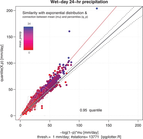
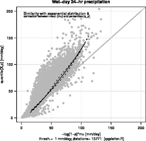
Figure 2 demonstrates that the quantiles q _0.95 of the wet-day 24-hr precipitation to some extent can be specified by its wet-day mean µ. Moreover, the qq-plot shows that most of the points are concentrated along the diagonal, suggesting that the statistical distribution for the 24-hr precipitation to a zeroth order is approximately exponential for virtually all of the rainfall records. However, the points exhibit a scatter around the diagonal, with a systematic bias for the high quantiles, where the empirical estimates tend to suggest a thicker upper tail in the distribution. Hence, the exponential will tend to underestimate the return values for the empirical rain gauge data. The points in Fig. 2 were colour coded with red for sites with low mean (wet + dry) precipitation and blue for sites with high mean precipitation. The dominance of red shading for low values and blue shading for high values is consistent with the quantiles being affected by the mean (wet + dry days) precipitation.

Fig. 2.  Quantile–quantile plot, plotting against the corresponding empirical estimate for estimated 95% quantile. The colour coding indicates the mean precipitation (wet + dry days). The data include GDCN for US stations as well as ECA&D, whose locations are shown in Fig. 1. The points are colour coded according to the 95th percentile estimated according to the mean (wet + dry) precipitation. The black-dashed lines are confidence intervals determined through Monte-Carlo simulations. Light grey contours show the point density.

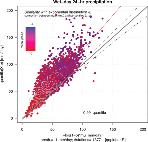
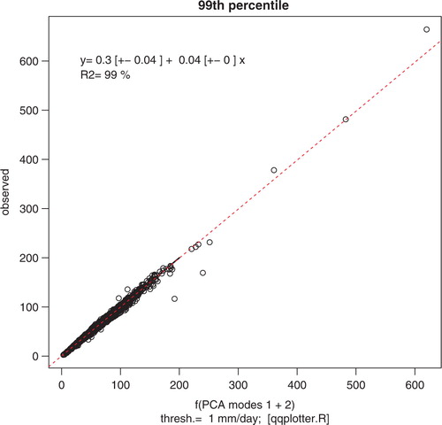
Figure 3 shows corresponding qq-plot for the 99th percentile, which exhibits a greater scatter than for the 95th percentile (Fig. 2). There are nevertheless clear hints of a dependency between these high percentiles and the wet-day mean µ. A linear regression analysis was used to compare quantile estimates assuming an exponential distribution, where against the empirical estimate. The regression analysis involved 14 different quantiles and rain gauge records from 13 771 locations, and the statistics describing the goodness of fit included R ²=0.95, f-statistic of 3.9×10⁶on 1 and 191 504 degrees of freedom, and a p-value <10⁻¹⁵.

Fig. 3.  Same as Fig. 2 but for the 99% quantile. The red line shows a linear best fit to the points based on linear regression. A cutoff of 200 mm d^–1 was used here, and for 8 locations the 99% quantile exceeded this limit (Fig. 5).

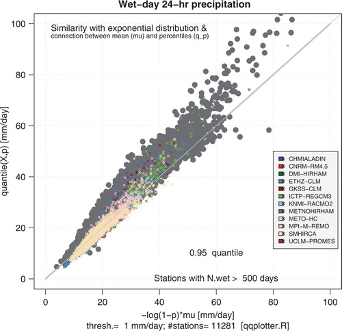
Figure 4 shows a similar analysis as Fig. 2 but for RCMs that are shown in different colours. As with the observations, the RCMs are scattered around the diagonal, suggesting a distribution that is close to being exponential. The RCMs vary in the absolute magnitude of the quantiles (scale parameter) as well as in the wet-day frequency. A similar analysis applied to one of the RCMs (HadRCM3) with spatial resolution of 25 and 50 km, respectively (not shown), also suggests that the shape of the distribution of the 24-hr precipitation from the RCMs is robust.

Fig. 4.  Same as Fig. 2, but contrasting results from the ENSEMBLES RCMs against corresponding analysis based on European ECA&D data (grey symbols). Only the rain gauge data with quantiles of similar range as the RCMs are shown.

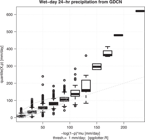
Although Fig. 2 shows a cloud of all the data points, it does not convey any information about the density of the points, as they may mask each other. Figure 5, on the other hand, shows a quantile–quantile boxplot, for which the boxes describe the interquartile range (mid 50% of the points) of the points in the qq-plot. This figure includes a range of quantiles (p∈[0.50,  0.55, …,  0.95] and p∈[0.96,  0.97,  0.98,  0.99]). The interpretation is more complicated for a range of quantiles and stations with different values for µ and q _p . However, the inclusion of a range of probabilities makes the results more general, as variables following the exponential distribution are expected to produce points on the diagonal regardless of the level of probability.

Fig. 5.  X-y boxplot plotting against the corresponding empirically estimated quantile. The plot shows a range of different quantiles, from 50% to 99%. The boxes deviating strongly from the diagonal above 200 mm d^–1 represent 18 of the quantiles found from the observations, representing only 8 locations.

A PCA of the cloud of points in the qq-plot in Fig. 5 produced a leading mode describing a smoothly varying function (Fig. 6). Likewise, the second mode had a smooth shape with a different curvature. Despite the scatter of points in Figs. 5 and 6, the qq-box plots and the PCA suggest that the quantiles q _p of the 24-hr precipitation is not far from being exponential for different values of p, albeit with a growing systematic bias for higher values. The points diverging away from the diagonal for 24-hr precipitation amounts greater than 200 mm d⁻¹ represent only eight locations.

Fig. 6.  The leading mode of the PCA of the points in Fig. 5 (black solid line) is shown on top of the cloud of points (grey) from all the GDCN stations (N=13549), whereas the dashed lines show the effect of the second mode (mode 1 ± mode 2).

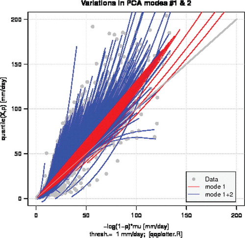
The two leading modes could reconstruct most of the scatter seen in Figs 2 and 3 (Fig. 7). Whereas the leading PCA mode (red lines) only seems to describe the main ‘axis’ of the cloud, the sum of the first and second mode (blue) appears to account for most of the spread of the points. The eigenvalues from the PCA suggested that the leading mode explained 99.4% of the total variance, and an independent linear regression analysis between data represented by the grey points in Fig. 7 and the red lines yielded an R ²-statistic of 0.98. Hence, the red lines in the figure provide a close description of the 14 quantiles between the 50% and 99% levels for the vast majority of the rain gauge records.

Fig. 7.  Reconstruction of the spread in the qq-plot from the two leading PCAs X=α _i E, where index i refers to the station number. A linear regression analysis between the grey points in the scatter plot and the leading PCA mode (red curves) suggests that the leading mode could reproduce 98.4% variance. A similar regression analysis applied to the sum of the two leading PCA modes (blue curves) explained 99.7%.

The sum of the two leading modes of the PCA can reproduce with even higher accuracy quantiles up to q _0.99. A linear regression analysis between the values represented by the blue curves and the grey points gave an R ²-statistic of 99.7%. Figure 8 shows a scatter plot between q _0.99 derived from two PCA modes and observed values. Here, the set of quantiles was estimated according to , and the value for q _0.99 was extracted from the vector, taking the value in Z with the index corresponding to the observed 99th quantile (see the appendix for more details). A linear regression analysis suggested that the leading mode by itself could account for 93.1% of the variance, for 13 768 degrees of freedom and a virtually zero p-value. A reconstruction of q _0.99 based on the sum of PCA modes 1 and 2, on the other hand, gave an R ²-value of 99.4%.

Fig. 8.  Scatter plot showing values for q _0.99 from observations compared with corresponding reconstructed values based on modes 1 and 2 from the PCA. The red dashed line shows the best fit based on a regression analysis.

An interesting question is whether the PC loadings, one for each station, exhibit any systematic pattern in terms of geographical location. A multiple regression analysis of the PC loadings of the leading mode indicated a strong relationship with mean (wet + dry day) precipitation, altitude, latitude and longitude (p-value less than 10⁻¹⁵ for all these), and a regression analysis can account for 65% of the variance (adjusted R ²). The regression analysis did not include the mean 2-metre temperature [T(2m)] or mean sea-level pressure that also may have an effect on these shapes, although the effect of T(2m) is expected to co-vary with the altitude and latitude. Figure 9 shows a map of the geographical distribution of the PC loadings of the leading mode.

Fig. 9.  Map showing the distribution of the leading PC loadings. No scale is given to the colourbar, as the value of the PC loadings is meaningless without the other components of the PCA (eigenvalue and mode).

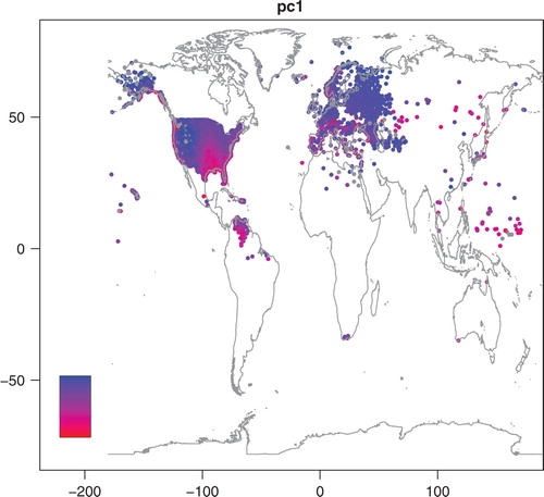
The same regression analysis for the second PCA mode, on the other hand, could only associate with 15% of the variance (not shown), but the same geographical parameters that were important for the leading mode also exhibited a close link to the second mode.

4. Discussion

Rain is a product of several different phenomena, such as fronts, nimbostratus, cyclones, convective clouds, and orographic forcing. The micro-physics of rain initiation may involve a cascading avalanche through collision and coalescence (Blyth et al., 1997), conditioned by the larger scale environment (Rogers and Yau, 1989). Wilson and Toumi (2005) provided a simple and elegant description of precipitation in terms of horizontal convergence of moisture flux, but their simple model did not resolve more complicated situations, such as multiple updraught from a single precipitating ascent. They nevertheless observed a remarkable uniform character in the precipitation characteristics, arguing that the data should follow a stretched exponential. Here, the empirical precipitation data from USA and Europe also exhibit a uniform behaviour in terms of belonging to one family of curves that for some purposes can be approximated as being exponential.

Assuming a simple exponential distribution allows a rule-of-the-thumb estimation of higher percentiles, albeit with some biases. The higher the quantile, the greater the bias. More sophisticated methods will provide a more accurate description of the upper tails of the rainfall distributions, and we have shown that a simple PCA, based on the assumption that the data approximately follow an exponential distribution, can explain most of the variance in its two leading modes. An exploration of the PCA products, furthermore, suggests that 65% of the variance of the leading PC and 15% of the second PC can be predicted from information about the stations’ geographical situation and can, hence, be used to provide a refined description of the upper quantiles. One interesting question is whether it is possible to predict the remaining part of these PC loadings.

Wilson and Toumi (2005) suggested that the stretched exponential shape is unlikely to change under a climate change. If this means that if the shape approximately similar to the exponential found in the present data does not change, then a change in upper quantiles in the future too will be closely related to the wet day mean µ, and would, furthermore, be in qualitative agreement with higher quantiles changing disproportionally compared to lower ones, as proposed by Semenov and Bengtsson (2002) and Frei et al. (2006).

These results also support the findings of Benestad (2007, 2010) in the sense that the distribution is approximately exponential, and that the quantiles exhibit a systematic relationship with the mean (wet + dry days) precipitation. Benestad (2007) also related the rate of the exponential (m in e ^mx where m < 0) to the mean 2-metre temperature and (wet + dry day) precipitation. Although this latter relationship was not examined further here, there is some support for the link between the mean (wet + dry day) precipitation and the quantiles, as seen in the colour coding in Figs. 2 and 3. It is also possible that µ and m are related to the mean sea-level pressure, as high-pressure regions tend to be associated with dry climates with blue skies (sub-tropics, the Azores high), whereas low-pressure regions often are near the storm tracks.

This study focused on the wet-day distribution of the precipitation, but to provide useful return values and intervals, it is important to also include the wet-day frequency. The total rain amount can be described in terms of a Bayesian probability , where f is the p.d.f. for the wet-day amount and g(r) is the probability of a wet day. The probability for rain g(r) is related to cloudiness, and hence correlates with temperature, depending on the situation. The question of causality is furthermore ambiguous: Hot temperatures favour convection during summer, whereas summertime stratocumulus clouds block the sun.

Our results do not necessarily disagree with the conclusion of Orskaug et al. (2011), as here we compared the 24-hr precipitation distribution with an exponential distribution. The analysis presented in Figs 2–4 suggests that the RCMs simulate lower values for the higher quantiles than seen in the observations (the grey points are further up the diagonal). But, it is also important to keep in mind that the representation of precipitation in RCMs is different to observations, as the former describes an area mean, whereas the latter is more a point measurement. A better way to assess the RCM results would be to compare them with gridded precipitation analyses such as E-OBS (Haylock et al., 2008; van den Besselaar et al., 2011).

Our findings are also qualitatively in good agreement with Wilson and Toumi (2005), even though it is not entirely clear to us that their assertion is valid. Their thesis builds on Frisch and Sornett's (1997) which states that stretched exponential p.d.f.s can arise because of an underlying random multiplicative processes, where the upper tail of the p.d.f. is produced from the sum of a finite number of independent random variables with a common p.d.f. e^−f(x) . Wilson and Toumi (2005) argued that the precipitation total (where is the instantaneous precipitation efficiency, is the mean specific humidity or mass mixing ratio, and m is the mass of air advected into the column and pushed through the moist level) and assumed these to be normal variables with similar p.d.f.s. Monte-Carlo simulations involving taking the product of three series of random normally distributed values (each with N=100 000) suggest an unrealistic description of the lower quantiles and that the quantiles depend on the mean values of the different factors (not shown).

Another aspect to consider is the errors in the rain gauge measurements. Such errors are likely to affect the scatter and bias. Large sampling fluctuations are also expected at the very upper end of the tails. The effect of errors may be reduced using a large sample of stations and applying PCA, keeping only the two leading modes. The PCA may, furthermore, facilitate a more sophisticated method to provide a more accurate/precise estimates of return values than assuming an exponential distribution, yet making no assumption about the shape of the p.d.f.

A comparison between the PCA-based representation of quantiles presented here and other methods such as the gamma distribution, generalised Pareto distribution (GPD) or a mixture of these (Vrac and Naveau, 2007) could provide benchmarks about accuracy and precision. This is, however, beyond the scope of the present article. Frigessi et al. (2003) and Friederichs (2010) argued that selecting exceedance thresholds may be tricky, and the threshold levels will probably vary from location to location and merit a study by themselves. A comparison between best-fit exponential and gamma distributions was made by Benestad (2010), and it was mainly for the low percentiles that the different types diverged. Nevertheless, further comparisons and evaluations should be carried out in future studies.

5. Conclusions

The daily rainfall distribution is approximately exponential to a zeroth order, with a bias in the upper part of the tail. This characteristic seems to be universal over different regions of the world and in both empirical data and regional climate model results. This means that, to a zeroth order, quantiles for 24-hr precipitation can be specified from the wet-day mean according to , and hence it is possible to provide an approximate estimation of the 24-hr wet-day precipitation quantiles once the wet-day mean µ is known. However, the two leading modes from a PCA can be used to provide a more accurate representation of the daily rainfall distribution.

Acknowledgements

This work was carried out during a visit to NCAR, whose hospitality is gratefully acknowledged. The work was supported by the Norwegian Research Council travel grant (Project Number: 203866 ‘Empirical-Statistical Downscaling in USA’) and the Norwegian Meteorological Institute. We wish to acknowledge the valuable access to the GDCN data. The ENSEMBLES data used in this work were funded by the EU FP6 Integrated Project ENSEMBLES (Contract number 505539), whose support is gratefully acknowledged. We are also grateful for comments on the manuscript from Anita Verpe Dyrrdal and from constructive reviews from two anonymous reviewers.

Notes

¹ http://www.ncdc.noaa.gov/oa/climate/research/gdcn/gdcn.html

² http://eca.knmi.nl/

³Using the function quantile() in the R-environment.

⁴See appendix for details.

7. Appendix

A.1. Derivation of the analytical expression

The p.d.f. is used to describe the transform , i.e. the rainfall amounts exceeding a threshold value (here taken to be 1 mm d⁻¹). Let be the p.d.f. of variable (precipitation, which X' refers to here, cannot be negative). ThenA.1

We assume that X' follows an exponential distribution of the form , and the area under this curve is:A.2

The analytical expression for the percentiles can be found by solving the integral over the p.d.f.:A.3

An analytical expression for the mean value (µ) can be derived by employing integration by parts:A.4

By combining equations A.3 and A.4, we get the expression relating the percentiles to the mean value:A.5

A.2. Computation of PCA

The PCA was performed on a matrix Z containing the quantiles calculated according to and corresponding quantiles estimated through the R command ‘quantile(X′, p)’, where p = [p ₁, p ₂, … p _m ] .The PCA was performed on the quantiles without subtracting the mean values (often PCA are performed on anomalies rather than the total values). Each column of Z represented one rain gauge record (N rain gauges in total), and consisted of vectors constructed by concatenating the m values of q _p with corresponding m values of ‘quantile (X′, p)’. A singular vector decomposition (SVD) (Press et al., 1989) was applied to Z to compute the principal components: . We used eigenvectors scaled by the eigenvalue to represent the leading modes. The graphical presentation of the PCA modes involved splitting each mode into two components representing q  _p and ‘quantile (X′, p)’ respectively. The PCA was implemented using the qPCA() function in the qqplotter package.

The reconstruction of the individual quantiles was based on the expression , for which the columns of matrix Z can be regarded as a set of N vectors Z[z ₁, z ₂, … z _N ] . Each column z  _i contains both a set of quantiles according to and the corresponding observed values quantile(X′, p). Hence, the original quantiles can be reconstructed from PCA by taking the element in z  _i with the index that corresponds to quantile (X′, p).

A.3. Implementation

The analysis and figures presented here were made using the R-package ‘qqplotter’ (version 1.10) and the R-package ‘PrecipStat’ (version 1.00) that contain the data needed to get these results. Both these packages are free and open source and can be obtained from the CRAN web site: http://cran.r-project.org. These R-packages also include basic documentation about their functions. Most of the results presented in this paper were produced by the function call ‘qqplotter()’.

• Map of locations of the rain gauge data used in the analysis with number of wet-days greater than 1000. The points are colour coded according to the 95th percentile estimated according to .

• Quantile-quantile plot, plotting against the corresponding empirical estimate for estimated 95% quantile. The colour coding indicates the mean precipitation (wet + dry days). The data include GDCN for US stations as well as ECA&D, whose locations are shown in Fig. 1. The points are colour coded according to the 95th percentile estimated according to the mean (wet + dry) precipitation. The black-dashed lines are confidence intervals determined through Monte-Carlo simulations. Light grey contours show the point density.

• Same as Fig. 2, but for the 99% quantile. The red line shows a linear best fit to the points based on linear regression. A cut-off of 200 mm d⁻¹ was used here, and for 8 locations the 99% quantile exceeded this limit (Fig. 5).

• Same as Fig. 2, but contrasting results from the ENSEMBLES RCMs against corresponding analysis based on European ECA&D data (grey symbols). Only the rain gauge data with quantiles of similar range as the RCMs are shown.

• X-y boxplot, plotting against the corresponding empirically estimated quantile. The plot shows a range of different quantiles, from 50% to 99%. The boxes deviating strongly from the diagonal above 200 mm d⁻¹ represent 18 of the quantiles found from the observations, representing only 8 locations.

• The leading mode of the PCA of the points in Fig. 5 (black solid line) shown on top of the cloud of points (grey) from all the GDCN stations (N=13549), whereas the dashed lines show the effect of the second mode (mode 1 ± mode 2).

• Reconstruction of the spread in the qq-plot from the two leading PCAs , where index i refers to the station number. A linear regression analysis between the grey points in the scatter-plot and the leading PCA mode (red curves) suggests that the leading mode could reproduce 98% variance. A similar regression analysis applied to the sum of the two leading PCA modes (blue curves) explained 99.7%.

• Scatter-plot showing values for q _0.99 from observations compared with corresponding reconstructed values based on modes 1 and 2 from the PCA. The red dashed line shows the best fit based on a regression analysis.

• Map showing the distribution of the leading PC loadings. No scale is given to the colourbar, as the value of the PC loadings are meaningless without the other components of the PCA (eigenvalue and mode).

References

- Balakrishnan N. Basu A. P. The exponential distribution: theory, methods and applications. B.V. Publishers: Amsterdam, 1995
- Benestad, R. E. 2007. Novel methods for inferring future changes in extreme rainfall over Northern Europe. Clim. Res. 34, 195–210. 10.3402/tellusa.v64i0.14981.
- Benestad R. E. 2010. Downscaling precipitation extremes: correction of analog models through PDF predictions. Theor. Appl. Clim. 100, 1. 10.3402/tellusa.v64i0.14981.
- Benestad R. E. Chen D. Hanssen-Bauer I. Empirical-statistical downscaling. World Scientific Publishing: Singapore, 2008
- Blyth A. M. Benestad R. E. Krehbiel P. R. Latham J. Observations of supercooled raindrops in New Mexico summertime cumuli. J. Atmos. Sci. 1997; 54(4): 569–575.
- Bremnes, J. B. 2004. Probabilistic forecasts of precipitation in terms of quantiles using NWP model output. Monthly Weather Rev. 132, 338347. 10.3402/tellusa.v64i0.14981.
- Bretherton C. S. Smith C. Wallace J. M. An intercomparison of methods for finding coupled patterns in climate data. J. Clim. 1992; 5: 541–560.
- Coles S. G. An introduction to statistical modeling of extreme values. Springer: London, 2001
- Epstein P. R. Ferber D. Changing planet, changing health. University of California Press: Berkely and Los Angeles CA, 2011
- Frei, C, Schöll, R, Fukutome, S, Schmidli, J and Vidale, P. L. 2006. Future change of precipitation extremes in Europe: intercomparison of scenarios from regional climate models. J. Geophys. Res. 111, D06105. 10.3402/tellusa.v64i0.14981.
- Friederichs P. Statistical downscaling of extreme precipitation using extreme value theory. Extremes. 2010; 13: 109–132.
- Friederichs P. Hense A. Statistical downscaling of extreme precipitation events using censored quantile regression. Monthly Weather Rev. 2007; 135: 2365–2378.
- Frigessi A. Haug O. Rue H. A dynamic mixture model for unsupervised tail estimation without treshold selection. Extremes. 2003; 5: 219–235.
- Frisch U. Sornett D. Extreme deviations and applications. J. Phys. I. 1997; 7(9): 1155–1171.
- Giorgi, F, Diffenbaugh, N. S, Gao, X. J, Coppola, E, Dash, S. K and co-authors. 2008. The regional climate change hyper-matrix framework. Eos. 89(45), 445–456.
- Haylock, M. R, Hofstra, N, Klein Tank, A. M. G, Klok, E. J, Jones, P. D and co-authors. 2008. A European daily high-resolution gridded dataset of surface temperature and precipitation. J. Geophys. Res. 113, D20119. 10.3402/tellusa.v64i0.14981.
- Klein Tank, A. M. G, Wijngaard, J. B, Können, G. P, Böhm, R, Demarée, G and co-authors. 2002. Daily dataset of 20th-century surface air temperature and precipitation series for the European Climate Assessment. Int. J. Clim. 22, 1441–1453. Online at: http://eca.knmi.nl.
- Kundzewicz, Z. W, Mata, L. J, Arnell, N, Döll, P, Kabat, P. and co-authors. 2007. Climate change: impacts, adaptation and vulnerabilit. Contribution of Working Group II to the fourth assessment report of the intergovernmental panel on climate change. Cambridge University Press: CambridgeUK and New York, NY, USA.
- Lanzante J. R. Resistant, robust, and nonparametric techniques for the analysis of climate data. Theory and examples, including applications to historical radiosonde station data. Int. J. Clim. 1996; 16: 1197–1226.
- Legates, D. R and Willmott, C. J. 1990a. Mean seasonal and spatial variability in gauge-corrected global precipitation. Int. J. Clim. 10, 111–127.
- Legates D. R. Willmott C. J. Mean seasonal and spatial variability in global surface air temperature. Theor. Appl. Clim. 1990b; 41: 11–21.
- Maraun, D, Wetterhall, F, Chandler, R. E, Kendon, E. J, Widmann, M and co-authors. 2010. Precipitation downscaling under climate change: recent developments to bridge the gap between dynamical models and the end user. Rev. Geophys. 48, 10.3402/tellusa.v64i0.14981.
- Oreskes, N, Stainforth, D. A and Smith, L. A. 2010. Adaptation to global warming: Do climate models tell us what we need to know?. Philos. Sci. 77, 1012–1028. 10.3402/tellusa.v64i0.14981.
- Orskaug, E, Scheel, I, Frigressi, A, Guttorp, P, Haugen, J. E and co-authors. 2011. Evaluation of a dynamic downscaling of precipitation over the Norwegian mainland. Tellus. 63A, 746–756.
- Peterson T. Daan H. Jones P. Initial selection of a GCOS surface network. Bull. Amer. Meteor. Soc. 1997; 78(10): 2145–2152.
- Press W. H. Flannery B. P. Teukolsky S. A. Vetterling W. T. Numerical recipes in pascal. Cambridge University Press: Cambridge, 1989
- Pryor, S. C, School, J. T and Barthelmie, R. J. 2005. Empirical downscaling of wind speed probability distributions. J. Geophys. Res. 110, D19109.
- R Development Core Team. 2004. R: a language and environment for statistical computing. R Foundation for Statistical Computing, Vienna, Austria. ISBN 3-900051-07-0.
- Rogers R. R. Yau M. K. A short course in cloud physics3rd edn. Pergamon Press: Oxford, 1989
- Schmidli, J, Goodess, C. M, Frei, C, Haylock, M. R, Hundecha, Y and co-authors. 2007. Statistical and dynamical downscaling of precipitation: an evaluation and comparison of scenarios for the Alps. J. Geophys. Res. 112, D04105. 10.3402/tellusa.v64i0.14981.
- Semenov, V. A and Bengtsson, L. 2002. Secular trends in daily precipitation characteristics: greenhouse gas simulation with a coupled AOGCM. Clim. Dyn. 19, 123–140. 10.3402/tellusa.v64i0.14981.
- Smither J. C. Schulze R. E. A methodology for the estimation of short duration design storms in South Africa using a regional approach based on L-moments. J. Hydrol. 2001; 241(1–2): 42–52.
- Solomon, S, Quin, D, Manning, M, Chen, Z, Marquis,M. and co-authors. 2007. Climate change: the physical science basis. contribution of working group I to the fourth assessment report of the intergovernmental panel on climate change. Cambridge University Press: CambridgeUK and New York, NY, USA.
- Themeßl, M. J, Gobiet, A and Leuprecht, A. 2010. Empirical-statistical downscaling and error correction of daily precipitation from regional climate models. International J. Clim. 31, 1530–1544.
- Timbal B. Jones D. A. Future projections of winter rainfall in southeast Australia using a statistical downscaling technique. Climatic Change. 2008; 86: 165–187.
- van den Besselaar, E. J. M, Haylock, M. R, van der Schrier, G and Klein Tank, A. M. G. 2011. A European daily high-resolution observational gridded data set of sea level pressure. J. Geophys. Res. 116, D11110. 10.3402/tellusa.v64i0.14981.
- van der Linden, P. and Mitchell, J. F. B. 2009. Ensembles: climate change and its impacts: summary of research and results from the ENSEMBLES project. European Comission: Met Office Hadley CentreExeter, UK.
- Vrac, M and Naveau, P. 2007. Stochastic downscaling of precipitation: from dry events to heavy rainfalls. Water Resour. Res. 43, W07402. 10.3402/tellusa.v64i0.14981.
- Wilks D. S. Multisite generalization of a daily stochastic precipitation generation model. J. Hydrol. 1998; 210(1–4): 178–191.
- Wilks D. S. Interannual variability and extreme-value characteristics of several stochastic daily precipitation models. Agr. Forest Meteorol. 1999; 93(3): 153–169.
- Wilson, P. S and Toumi, R. 2005. A fundamental probability distribution for heavy rainfall. Geophys. Res. Lett. 32, L14812. 10.3402/tellusa.v64i0.14981.
- Woolhiser D. A. Roldán J. Stochastic daily precipitation models: 2. A comparison of distributions of amounts. Water Resour. Res. 1982; 18(5): 1461–1468.