Four-dimensional variational data assimilation for a limited area model

ABSTRACT

A 4-dimensional variational data assimilation (4D-Var) scheme for the HIgh Resolution Limited Area Model (HIRLAM) forecasting system is described in this article. The innovative approaches to the multi-incremental formulation, the weak digital filter constraint and the semi-Lagrangian time integration are highlighted with some details. The implicit dynamical structure functions are discussed using single observation experiments, and the sensitivity to various parameters of the 4D-Var formulation is illustrated. To assess the meteorological impact of HIRLAM 4D-Var, data assimilation experiments for five periods of 1 month each were performed, using HIRLAM 3D-Var as a reference. It is shown that the HIRLAM 4D-Var consistently out-performs the HIRLAM 3D-Var, in particular for cases with strong mesoscale storm developments. The computational performance of the HIRLAM 4D-Var is also discussed.

The review process was handled by Subject Editor Abdel Hannachi

• data assimilation
• analysis
• numerical weather prediction

1. Introduction

The 4-dimensional variational data assimilation (4D-Var) was first suggested by Le Dimet and Talagrand (1986) and Lewis and Derber (1985). The idea of 4D-Var is to use observations over a finite time interval to compute an optimal initial state for a numerical weather prediction (NWP) model. The model initial state is obtained by minimising a cost function, which consists of one term measuring the distance between the 3-dimensional model initial state and a model background state at the beginning of the assimilation window, and another term measuring the distance between the observations distributed over the assimilation window and the corresponding model state values evaluated in the observation points. This article is concerned with the 4D-Var for the HIgh Resolution Limited Area Model (HIRLAM) forecasting system (Undén et al., 2002). The HIRLAM 4D-Var also includes optional cost function terms, one term to damp high-frequency oscillations, one term used for the control of lateral boundary conditions, one model error term (not yet validated) and one large-scale constraint term (Dahlgren and Gustafsson, 2012).The review process was handled by Subject Editor Abdel Hannachi

One of the most important aspects of 4D-Var is its implicit flow-dependent assimilation structure functions (Thépaut et al., 1996). 4D-Var takes the time dimension into account through the forecast model. Inclusion of the forecast model into the data assimilation process makes it possible to assimilate not only forecast model state variables but also diagnostic quantities, for example, surface pressure tendency and precipitation intensity. It is also possible to assimilate efficiently observations with a high resolution in time. Examples are surface observations, radar observations and ground-based Global Positioning System (GPS) observations. At horizontal resolutions of a few kilometre, the model-generated structure functions are probably much more important than any explicit balance constraints specified for the background term. There are no such obvious balance constraints known that can be applied to the convective storm scales, and thus 3-dimensional methods like 3D-Var will be less efficient in the mesoscale.

4D-Var provides us with the possibility to avoid an explicit initialisation at the start of the forecast to be run from the analyses. This is made possible through the application of a weak ‘initialisation’ constraint in the 4D-Var procedure. One such constraint, the weak digital filter constraint (Gustafsson, 1992; Gauthier and Thépaut, 2001), is discussed in this article. 4D-Var may also reduce the spin-up of physical processes during the first hours of the forecast. This necessitates, in addition, the application of reasonably realistic physical parameterisations [in the tangent linear (TL) and adjoint (AD) models].

One basic weakness of 4D-Var is the assumption of a perfect forecast model over the assimilation window – the forecast model is applied as a strong optimisation constraint. However, there exist possibilities to partly compensate for this weakness of 4D-Var. The original idea of Lewis and Derber (1985) to use some quantity representing model errors, for example, a tendency bias, in the assimilation control vector has recently received renewed interest (Trémolet, 2006) and can be applied also in the HIRLAM 4D-Var.

The incremental 4D-Var approach (Courtier et al., 1994) is based on a linearisation of the forecast model equations around a model trajectory being sufficiently close to the true development of the atmosphere, such that the resulting analysis would be within the estimation error of the truth. It may be argued that such linearisations are impossible, or very difficult, when taking strongly non-linear processes like convection into account. It may be necessary to introduce the different spatial scales and the different processes step-wise into the minimisation, starting with quasi-linear near-adiabatic synoptic scale processes and introducing smaller scales and physical processes gradually. For this purpose, there must be access to a range of regularised and simplified TL and AD physical parameterisation schemes that can be applied during different phases of the minimisation.

Another weakness of 4D-Var in its original formulation is the lack of flow dependency of the assimilation structure functions at the start of the assimilation window. Ensemble assimilation techniques, like the Ensemble Kalman Filter (Evensen, 1994), provide a natural framework for introducing such flow dependency. Hybrids between variational and ensemble assimilation techniques (Wang et al., 2007) have recently been applied with promising results. A hybrid variational ensemble data assimilation scheme, using the augmentation of the assimilation control variable suggested by Lorenc (2003), has also been developed for HIRLAM and will be described in a separate article.

An operational 4D-Var coupled to a spectral mesoscale model was introduced at the Japan Meteorological Agency (JMA) in March 2002 (Kawabata et al., 2007). The JMA 4D-Var has many characteristics in common with the HIRLAM 4D-Var: the spectral model formulation, the control of the lateral boundary conditions and the use of the National Metorological Center, the former name of the National Center for Environmental Prediction, Washington, USA (NMC) method for background error statistics.

The formulation of the HIRLAM 4D-Var is presented in Section 2, followed by an example of implicit dynamical structure functions in Section 3 using simulated observation experiments. The model setup for real observation experiments is then described in Section 4. Some sensitivity experiments regarding the weak digital filter constraint and the settings for the multi-incremental minimisation are presented in Sections 5 and 6, respectively. Results from pre-operational testing of HIRLAM 4D-Var and comparison with 3D-Var are provided in Section 7. These tests preceded the operational introduction of HIRLAM 4D-Var at the Swedish Meteorological and Hydrological Institute (SMHI) in January 2008. The computational efficiency of the HIRLAM 4D-Var is discussed in Section 8 and some concluding remarks are given in Section 9.

2. The HIRLAM 4D-Var formulation

The first step in the development of HIRLAM 4D-Var was the adiabatic Eulerian TL and AD models and the application to studies of sensitivity of forecast errors to initial states and lateral boundaries (Gustafsson and Huang, 1996; Gustafsson et al., 1998). The AD model was also used to improve the Optimal Interpolation-based HIRLAM data assimilation system at that time (Huang et al., 1997). Further developments of the HIRLAM 4D-Var (Huang et al., 2002) included the incremental formulation proposed by Courtier et al. (1994), applied also in HIRLAM 3D-Var (Gustafsson et al., 2001; Lindskog et al., 2001) and the implementation of the simplified physics packages from European Centre for Medium-range Weather Forecasts (ECMWF) (Buizza, 1993) and Météo-France (Janisková et al., 1999). Later developments include the multi-incremental formulation following Veersé and Thépaut (1998), the semi-Lagrangian time integration following Hortal (2002), the use of grid point HIRLAM forecasts for the 4D-Var background, the weak digital filter constraint following Gustafsson (1992) and the control of lateral boundary conditions following the JMA approach (Kawabata et al., 2007).

The HIRLAM 4D-Var utilises Fourier transforms in the TL and AD models as well as in the background error constraint calculations. An area extension, suggested by Haugen and Machenhauer (1993), is applied in order to make assimilation increments periodic in both horizontal directions. Details on this area extension have been presented by Gustafsson et al. (2001).

2.1. The multi-incremental formulation

A fundamental problem in the application of 4D-Var is the non-linearity of the forecast model and the related risk for finding a local rather than the global minimum by a straightforward minimisation of the cost function J. It can be argued that variations of assimilation increments for near-adiabatic larger scale flow over an assimilation window of 6–12 h are more accurately approximated under assumptions of model linearity than the corresponding variations of assimilation increments for smaller scale diabatic flow. The basic idea of the multi-incremental approach is therefore to split the minimisation problem into a sequence of subproblems, where we first determine the minimum of the cost function for larger scale increments, with near-adiabatic processes included in the forecast model only and with a linearisation of the forecast model around a non-linear forecast starting from a model background initial state. Having determined these large-scale increments, it can be assumed that we are closer to the global minimum of the original minimisation problem and we can introduce smaller spatial scales and more diabatic processes step by step. In each step, we will relinearise the forecast model equations around the non-linear model trajectory starting from the improved initial state found in the previous minimisation step. With exception for the effects of variational quality control (VarQC) (see Lindskog et al., 2001), this relinearisation procedure guarantees that each minimisation subproblem remains a quadratic minimisation problem. This sequence of minimisation subproblems is often referred to as the ‘outer minimisation loop’ in 4D-Var, while the solution of each minimisation subproblem is referred to as an ‘inner minimisation loop’.

Let x ₀ denote the model initial state to be determined at time t  =  t ₀ at the beginning of the data assimilation interval, the corresponding background model state and the total assimilation increment. The total assimilation increment δx₀ is determined as a sum of assimilation increment contributions

where the contributions are determined through the solution of a sequence of quadratic minimisation problems for τ = 1,2, … ,N _τ, with N _τ being the number of outer minimisation loop iterations. Considering the background and observation error constraints, the cost function for determination of is defined by

where

with

here, M _k denotes a non-linear forecast from time t ₀ until time t _k , and H denotes a non-linear observation operator. and H ^τ−1 denote a TL forecast from time t ₀ until time t _k and a linear observation operator, respectively, both obtained by linearisation of the corresponding non-linear model and observation operator around the non-linear forecast starting from for t = 1 and from

for t > 1, y _k denotes the vector of observations available at time t _k , B a matrix containing covariances of background errors and R a matrix containing covariances of observation errors.

For application of a standard minimisation software package (for example Gilbert and Lemaréchal, 1989), the gradient of J with respect to the increment is needed. This gradient is given by

where denotes the AD of the TL model and the AD of the TL observation operator H ^τ−1. The gradient is calculated through a single integration of the TL model forward in time over the assimilation time window, followed by a backward integration of the AD model over the same time interval.

The spatial resolution of the contribution to the assimilation increment can gradually increase for each outer loop iteration, and the TL forecast model can be designed to include more and more complex physical processes with increasing outer loop minimisation iteration number. One particular feature of the HIRLAM 4D-Var is that the non-linear model may be either the grid point HIRLAM with a finite difference formulation or the spectral HIRLAM based on the spectral transform technique, while the TL model and the AD of the TL model are always based on the spectral model formulation. The non-linear model integrations are carried out with full model resolution for each outer loop iteration, and the resulting model trajectories are used at full resolution for calculation of J _o contributions and, after truncation, for the linearisations related to the TL and AD models. This approach was chosen in order to have the best possible model trajectory to be used for the linearisations.

To simplify the notations, we have dropped the index τ − 1, denoting the outer loop iteration number of the non-linear model state used for linearisation, in the descriptions and discussions of and H ^τ−1 below.

2.2. The background error constraint

The main purpose of the variational data assimilation background constraint is to force assimilation increments to obey balance relations and spatial spectral characteristics in accordance with statistical information on forecast background errors. The background error constraint of the HIRLAM 4D-Var is a modified version of the background error constraint described by Berre (2000). An f-plane balance based on a constant Coriolis parameter f ₀ is applied by Berre, while a balance operator based on a spatially variable Coriolis parameter f is applied in HIRLAM 4D-Var as well as in HIRLAM 3D-Var.

The large dimension of the background error covariance matrix B makes it difficult to store and it is practically impossible to compute B ⁻¹ by matrix inversion in grid point space. Furthermore, for the minimisation to converge rapidly, a pre-conditioning is necessary. The ideal pre-conditioning is to transform the increment into a control variable such that the Hessian matrix of the cost function J becomes the identity matrix. For the HIRLAM 3D-Var we have introduced a control variable transform χ = Uδx ₀ , making it possible to assume that the Hessian matrix of the background error constraint J _b is an identity matrix. This is a good pre-conditioning as long as the Hessian of J _b is large compared to the Hessians of the other cost function contributions. Two main assumptions built into the control variable transform of the HIRLAM 3D-Var are those of horizontal homogeneity with respect to horizontal correlations, making the correlation matrix of a single 2-dimensional field diagonal in spectral space and the decoupling vertically through projection on eigenvectors of vertical correlation matrices. The transform U is defined: U  =  PVLSGF where F is the Fourier transform to spectral space, G is the balance operator based on statistical regression techniques (Berre, 2000), S is the normalisation with the background error standard deviations, L is the normalisation with the square roots of the horizontal spectral correlation density functions of forecast errors, V is the projection on the eigenvectors of the vertical forecast error correlation matrices and P is the normalisation with the square roots of the eigenvalues of the vertical forecast error correlation matrices. Note that the background error standard deviations are specified separately and preserved for different horizontal increment resolutions, which means that the horizontal spectral correlation densities have to be renormalised when horizontal resolution is changed. The forecast error statistical parameters are computed using the NMC method (Parrish and Derber, 1992). In connection with introduction of the multi-incremental minimisation, the question arose of which control variable to transfer between the different outer loop minimisation iterations. It turned out that neither the transformed control variable χ nor the analysis increment δx₀ in grid point space could be used. The transformed variable χ includes a normalisation with the square root of the horizontal spectral density function, which is resolution dependent. χ, therefore, cannot be used when the resolution is changed between the outer loop iterations, nor can the grid-point increment δx₀ be used because the Fourier transform back to the spectral space control variable space is non-unique. The non-uniqueness of the direct Fourier transform is due to the use of an extension zone to obtain bi-periodic variations in both horizontal dimensions. The applied solution is to transfer a ‘half-way’ transformed control variable L ⁻¹ V ⁻¹ P ⁻¹ χ between the outer loop minimisation iterations.

The assimilation control variables in the reference HIRLAM 4D-Var and 3D-Var are vorticity, unbalanced divergence, unbalanced temperature, unbalanced surface pressure and unbalanced specific humidity. For the humidity analysis, a renormalised pseudo-relative humidity assimilation control variable may also be applied (Gustafsson et al., 2011). The renormalisation follows Hólm et al. (2002), and the purpose is to improve Gaussianity close to zero humidity and saturated model background states. Since the renormalisation has a non-linear formulation, several outer loop minimisation iterations are required (Gustafsson et al., 2011).

2.3. Observation operators, observation error covariances and VarQC

The observation operators include the non-linear operator H, the TL operator H and the AD operator H ^T . Each observation operator generally includes a horizontal interpolation of the model state to observation geographical locations, a calculation of pressures and geopotentials at model levels (at the observation locations), a vertical interpolation of the model state to observation altitudes and specialised operators for each type of observation.

To compute the observation constraint, the observation error covariance matrix R is needed. Both instrument errors and representativeness errors are represented in R. Just like in the HIRLAM 3D-Var, we assume observation errors to be uncorrelated and only the error standard deviations enter into R. For the observed values from conventional data types and their associated error standard deviations, we use the same procedures as in the HIRLAM 3D-Var (Lindskog et al., 2001). The conventional observations include synoptic observations (SYNOP), ship observations (SHIP), buoys (BUOY), pilot balloons (PILOT), radiosondes (TEMP) and aircraft reports. In addition, the ATOVS AMSU-A radiance data over seawater areas have been used in this study (Schyberg et al., 2003).

The HIRLAM 4D-Var has been applied to the assimilation of clear and cloud-affected SEVIRI radiances by Stengel et al. (2009, 2010), and in this work the renormalised pseudo-relative humidity assimilation control variable and several outer loop iterations were applied successfully.

The VarQC accounts for the possibility of gross errors, represented by a flat Probability Density Function (PDF), in addition to random errors, represented by a Gaussian PDF (Andersson and Järvinen, 1999). The VarQC is only applied during a sequence of iterations between two specified iteration numbers of the HIRLAM 4D-Var minimisation. Observed values considered as rejected by the end of this sequence of iterations are left out from the remaining part of the minimisation iterations in order to stay with a quadratic minimisation problem (for details see Lindskog et al., 2001).

All observed values that enter into the HIRLAM 4D-Var minimisation have also been subject to a number of stand-alone quality control algorithms like comparison with a short range forecast background value. These (screening) quality control algorithms are the same as those applied in HIRLAM 3D-Var (Lindskog et al., 2001).

2.4. Assimilation forecast models

The non-linear forecast model M is used to propagate the background model state, as well as subsequent analysis guess fields in the outer minimisation loop, forward in time, the TL model M _k is used to propagate the analysis increments forward in time, while the AD model is used to propagate the gradients of the cost function with respect to the model state variables backward in time. The operational version of the HIRLAM forecast model is based on a grid point representation for model variables, approximation of spatial derivatives by second-order finite differences and a semi-implicit time stepping (Undén et al., 2002). However, the spectral version of the HIRLAM forecast model is also available (Gustafsson, 1991; Gustafsson and McDonald, 1996).

The Eulerian version of the spectral HIRLAM was chosen as the basis for the development of the TL and AD models (M _k and ), mainly due to practical reasons (Gustafsson and Huang, 1996); for example, the Fourier transforms are self-AD, and the ADs of complicated finite difference expressions are avoided. A manual coding technique was used statement by statement, block by block and subroutine by subroutine. The following steps are needed: (1) Coding of the TL counterpart of the non-linear code; (2) By considering each TL code statement as a complex valued matrix operator, the AD code statement is derived by taking the complex conjugate and transpose of it; (3) The correctness of AD code is checked. If the AD code has been formulated correctly, the following should hold up to the machine accuracy:

(4) Finally, to test the validity of the TL approximation, gradient tests are performed on selected TL components and the full TL model:

For values of α which are small but not too close to zero at machine accuracy, the above value is expected to be close to unity.

2.4.1. Semi-Lagrangian time integration in the TL and AD models.

To improve the computing performance of HIRLAM 4D-Var, semi-Lagrangian versions of the TL and AD HIRLAM spectral models were developed. The semi-Lagrangian scheme of the original spectral HIRLAM model (Gustafsson and McDonald, 1996) was modified along the ideas of the ‘Stable Extrapolation Two-Time-Level Scheme (SETTLS)’ described by Hortal (2002). This semi-Lagrangian scheme provided a significant performance improvement due to less severe restrictions on the time-step and due to a cleaner two-time-level formulation, avoiding the need for any time filter.

The basic idea of the SETTLS semi-Lagrangian scheme is to expand any unknown model quantity in a second-order Taylor series around the departure point of the semi-Lagrangian trajectory at time t, including an estimation of the second-order term through averaging along the backward trajectory between time t–Δt and time t. For the implementation of this scheme into the spectral HIRLAM, we followed the model equations described by Gustafsson and McDonald (1996) and the numerical scheme of Hortal (2002) closely. A linear 3-dimensional interpolation scheme is used in the calculation of model trajectories and for non-linear quantities, while a 3-dimensional cubic interpolation scheme is used for all basic model quantities that are subject to the semi-Lagrangian interpolation. The semi-Lagrangian scheme is combined with a semi-implicit time integration (for details see Gustafsson and McDonald, 1996).

The TL and AD of semi-Lagrangian time integration schemes were discussed by Polavarapu et al. (1996). The main issue is that the interpolation, needed to fetch various quantities along the backwards trajectories in the semi-Lagrangian scheme, is not differentiable unless we restrict the interpolation in the linearised scheme to use values from the same set of grid points that is used in the corresponding non-linear scheme. In other words, even if the trajectory perturbed by the TL wind increment indicates that we should move to a new set of grid points for the interpolation, we should still use the set of grid points determined by the unperturbed trajectory.

Starting from the requirement for differentiability, the development of the TL and AD semi-Lagrangian schemes for HIRLAM 4D-Var was a straightforward task. The TL trajectory calculation provides TL (perturbed) trajectory displacements and the TL semi-Lagrangian interpolation, the needed TL (perturbed) quantities. Similarly, the AD semi-Lagrangian interpolation and trajectory calculations provide links from gradients of increments in the interpolated quantities to gradients of increments in the grid point fields as well as gradients of increments in the wind field used for the trajectory calculations.

From a numerical stability point of view, due to the linearisation of the interpolation scheme, the TL and the AD of the semi-Lagrangian scheme act more like an Eulerian scheme than a semi-Lagrangian scheme. It is the magnitude of the wind increment that determines the stability for any particular case. For this reason, it is computationally favourable to utilise the multi-incremental minimisation formulation by letting outer loop iterations at coarser resolution to determine a larger fraction of the assimilation increments.

2.4.2. The TL and AD model physics

Due to the incremental formulation of the HIRLAM 4D-Var, it is also reasonable to simplify the linearised (TL and AD) HIRLAM physics or even to utilise other linearised physics packages.

One of the ECMWF simplified physics packages (Buizza, 1993), referred to as the Buizza scheme here to distinguish it from other ECMWF simplified physics packages, was chosen due to its extreme simplicity. The scheme contains only a very simple representation of vertical diffusion of momentum and surface friction. The Météo-France Simplified Physics package contains a series of simplified computations of radiation, vertical turbulent diffusion, orographic gravity wave drags, deep convection and stratiform precipitation fluxes (Janisková et al., 1999). The individual physics contributions in this package can be computed independently, thus the need for extra array storage and partial recalculation of non-linear steps in physics AD subroutines are drastically reduced compared to the case using, for example, the TL and AD of the full HIRLAM physics (Yang, 2002). For the experiments reported on in this article, only the turbulence parameterisation of the Janisková et al. (1999) package has been applied, since it is a more complete turbulence scheme than the Buizza (1993) scheme that treats vertical turbulent exchange of momentum only. The large-scale condensation scheme of Janisková has also been applied successfully for certain data periods with the HIRLAM 4D-Var but was not applied here because of a too strong tendency to trigger unrealistic small-scale instabilities.

2.5. The weak digital filter constraint

Numerical weather prediction models based on the primitive equations describe slow Rossby modes as well as fast gravity modes. While the former are of main meteorological interests, the latter are only associated with small amplitude in the atmosphere as measured, for example, by the kinetic energy power spectrum of the gravity modes. When fitting a model trajectory to observations, as formulated in 4D-Var, we wish to modify the Rossby modes while minimising the amplitudes of fast gravity wave oscillations. Commonly used approaches to control the fast modes are to apply the Non-linear Normal Mode Initialisation (NNMI) scheme (Machenhauer, 1977) or the Digital Filter Initialisation (DFI) scheme (Lynch and Huang, 1992). The TL and AD of the NNMI have been introduced into the HIRLAM 4D-Var as well as a weak digital filter constraint. The weak digital filter formulation follows Gustafsson (1992) and Gauthier and Thépaut (2001). A term J _c is added to the 4D-Var cost function:1

with2

where δx _n is the model state assimilation increment at time-step n calculated from the initial state assimilation increment δx ₀ by the TL model δx _n =M _n δx₀, N is the number of time steps over the data assimilation window and is the digitally filtered assimilation increment at the mid-point of the data assimilation window. Note that N must be an even number. The parameter we will consider is a tuning parameter, describing the relative importance of the noise filtering constraint J _c in comparison with the observation error constraint J _o and the background error constraint J _b . The diagonal matrix C⁻¹ defines the relative weights given to different model variables at different vertical levels in the weak digital filter constraint and we have defined these in accordance with the total energy norm, with no horizontal variation of the integration weights (and with no horizontal resolution dependency of the horizontal weights). f _n , finally, are the digital filter weights. We have determined these in accordance with the Dolph filter (Lynch, 1997), which is defined by a time span (= the length of the data assimilation window = 5 h in our case) and a cutoff frequency period, T _c .

Using the reformulated digital filter weights (h _n ,n = 0,…,N), the digital filter cost function J _c and its gradient with respect to the initial time assimilation increment may be calculated as follows:3

and4

From the expression for the gradient , we can notice that the deviations from the digitally filtered model assimilation increment will enter as a forcing for the AD model equations (), similar to the way the deviations from the observations (as defined by J _o ) also enter as a forcing to the AD model equations.

The weak digital filter constraint is applied in inner minimisation loops of the HIRLAM 4D-Var only. We consider the constraint mainly as a tool to avoid fast gravity wave oscillations in the TL model integrations. Furthermore, it is not clear how one should apply the filter to the total assimilation increment over several outer loop iterations, since this total increment will include contributions also from the non-linear model trajectory runs between the outer loop iterations.

2.6. Implementation issues

The HIRLAM 4D-Var includes the HIRLAM 3D-Var as a component. There are a number of differences between 3D-Var and 4D-Var (assuming 6 h cycling and taking the analysis around 0000 UTC as an example):

Assimilation interval: For 3D-Var, the assimilation interval is 6 h, 21:00–02:59 h, but this is just a matter of definition. For 4D-Var, with a 6-h assimilation interval, 20:30–02:29 h may be chosen in order to have symmetric hourly observation windows. A centred 3-h assimilation interval, 22:30–01:29 h, or an uncentred 5-h interval, 20:30–01:29 h, may also be chosen. Overlaps of adjacent assimilation intervals should be avoided due to the risk of repeated use of observations.

Observation window: For 3D-Var, the observation window length may be freely chosen as long as no overlap of adjacent observation windows occurs. In the 3D-Var experiments described in this article, the observation window length was 6 h, 20:30–02:29 h. For 4D-Var, the observation window length is currently set to 1 h, but it can easily be changed. Six observation windows were used for the analysis: 20:30–21:29, 21:30–22:29, 22:30–23:29, 23:30–00:29, 00:30–01:29, 01:30–02:29 h. Note that the observation window 02:30–03:29 h is not included for this cycle in order to avoid repeated use of the same observations.

Background states: For 3D-Var, hourly background states are provided in order to minimise the model error influence on the innovations, which is sometimes referred to as First Guess at Appropriate Time (FGAT). For 4D-Var, hourly background states are also provided.

Analysis propagation: For 3D-Var, the full analysis state is propagated forward in time to the next analysis time by the non-linear forecast model, while with 4D-Var there is also an option to propagate the assimilation increment forward in time by the TL model to the start of the next assimilation window.

3. Implicit dynamical structure functions

A crucial component of all statistical analysis schemes is the background error covariance matrix, B. The B matrix determines the shape of the analysis increments and the degree of balances in the analysis. An efficient way to check a data assimilation scheme is to perform single simulated observation impact experiments. The analysis increments due to a single observation can directly be associated with the multivariate structure functions, that is a single row or column of B, and their flow dependencies in the case of 4D-Var. Single observation impact experiments with the ECMWF 3D-Var and 4D-Var were carried out by Thépaut et al. (1996). Based on the theoretical equivalence between 4D-Var and the Extended Kalman Filter (EKF) (Ghil and Malanotte-Rizzoli, 1991), the analysis increments from these experiments were used to investigate the dynamical structure functions implied in the ECMWF 4D-Var. It was shown that the implied ECMWF 4D-Var structure functions differ considerably from those of 3D-Var. The main features of 4D-Var such as flow dependency associated with baroclinic structures were demonstrated.

Single observation impact experiments with the HIRLAM 3D-Var have confirmed that the analysis increments are in accordance with the applied analysis structure functions and that the fit of the analysis to the observations is in agreement with the assumed background and observational error statistics (Gustafsson et al., 2001; Lindskog et al., 2001). Here, we used single observation impact experiments to investigate the structure functions implied by the HIRLAM 4D-Var increments.

We first derive a special solution for 4D-Var with only one outer loop iteration and with only one observation y at time t _k and with . Introducing and dropping the summation in the gradient calculation as well as the outer loop index, the cost function gradient becomes5

At the minimum, , and with H _k =HM _K we will have6

where we also have introduced the dual (or the observation space) solution (see Kalnay (2003) for an elegant proof of the equivalence of the two solutions). Multiplying with M _k we will get the solution at time t _k 7

where is the background error covariance matrix valid at time t _k , as provided by an EKF. Assuming that the single observation concerns model component j, denoted by , the solution for model component i is given by:8

which is the solution also given by an EKF. This means that the impact of a single observation at time t _k on the increment δx _k valid at time t _k is given by the flow-dependent background error covariance B _k , calculated in exactly the same way as through the EKF. In this sense, 4D-Var is equivalent to an EKF over the time period of the data assimilation window. We provide an example of these flow-dependent background error covariance matrices in the following, together with a discussion of their significance and a comparison with 3D-Var covariance matrices.

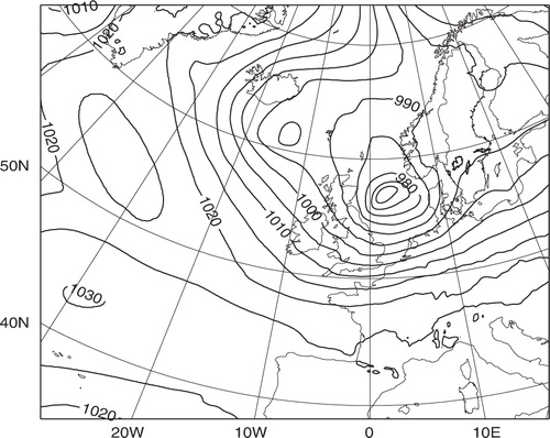
The case chosen is the severe cyclone of 3 December 1999, which crossed Denmark during the evening. We have selected the period between 06 UTC and 12 UTC, characterised by the strongest baroclinic development, for our experiment. The forecast background trajectory is produced by a HIRLAM non-linear model run with full physics from an interpolated ECMWF analysis at 00 UTC 3 December 1999. The simulated observations will be assimilated at 11 UTC, 5 h into the data assimilation window, and the 00 UTC +11 h background mean sea level pressure (MSLP) forecast is given in Fig. 1.

Fig. 1.  HIgh Resolution Limited Area Model mean sea level pressure (MSLP) forecast on 3 December 1999, 00 UTC + 11 h. The contour interval is 5 hPa.

First, we introduce a single simulated surface pressure observation increment of −5 hPa at 57°N 3°E, in the area with the fastest development of the storm. As a reference for the 4D-Var experiment, we first carry out a 3D-Var single simulated observation experiment. The result is presented in Fig. 2. As expected, we obtain an almost isotropic, rather large-scale, and completely flow independent, surface pressure increment. The deviations from isotropy in areas with elevated terrain can be explained by the use of the increment of the logarithm of surface pressure as the assimilation control variable.

Fig. 2.  3D-Var surface pressure assimilation increments for 3 December 1999, 11 UTC from a single surface pressure observation increment of −5 hPa at 57°N 3°E for 3 December 1999, 11 UTC. The assumed standard deviation of the observation error is 0.5 hPa. The contour interval is 1 hPa.

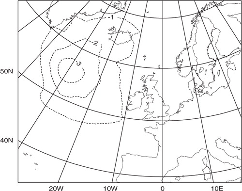
Second, we will use the same single simulated surface pressure observation in a 4D-Var experiment over the data assimilation window 06 UTC − 12 UTC. We will thus introduce the observation at the end of the data assimilation window, where we can expect the background error covariance to have been influenced by TL dynamics over 5 h of model integration time. The result of this experiment in the form of the surface pressure assimilation increments at 11 UTC is presented in Fig. 3. The main difference between the 3D-Var and the 4D-Var experiments is that the 4D-Var surface pressure increments at 11 UTC occur for much smaller horizontal scales, comparable to the horizontal scales of the core of the mesoscale storm development as seen in the non-linear forecast for the same time in Fig. 1. From this we may conclude that the implicit propagation of the background error covariance matrix over the data assimilation window provides information on preferred scales (and structures) of development as determined by the linearisation around the non-linear trajectory.

Fig. 3.  4D-Var surface pressure assimilation increments for 3 December 1999, 11 UTC, from a single surface pressure observation increment of −5 hPa at 57°N 3°E for 3 December 1999, 11 UTC. The data assimilation window is from 06 UTC until 12 UTC. The assumed standard deviation of the observation error is 0.5 hPa. The contour interval is 1 hPa.

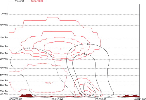
We may ask what perturbations at the start of the assimilation window are required to create the mesoscale storm perturbations as seen in the surface pressure assimilation increments 5 h later in Fig. 3. It turns out that the surface pressure assimilation increments at the start of the assimilation window (06 UTC) are quite small, while there exist significant wind and temperature assimilation increments at upper tropospheric levels, upstream of the storm development 5 h later. A vertical cross section of the 06 UTC wind and temperature increments in the NW–SE direction centred over the British Isles is presented in Fig. 4. The vertically tilted wind and temperature increments in this figure indicate an enhanced baroclinicity of the initial state for the TL model that 5 h later results in the intensified storm development. In other words, the most efficient initial change to provide an intensified storm development, as seen by surface pressure, is to change the upper air fields responsible for the enhanced dynamical development.

Fig. 4.  Vertical cross-section with 4D-Var assimilation increments of temperature and the wind component normal to the vertical cross-section at 3 December 1999, 06 UTC, from a single surface pressure observation increment of −5 hPa at 57°N 3°E with observation time 3 December 1999, 11 UTC. The data assimilation window is from 06 UTC until 12 UTC. The assumed standard deviation of the observation error is 0.5 hPa. The vertical cross-section extends from 67°N 25°W until 48°N 15°E. Contour intervals are 0.5 m s⁻¹ and 0.1 K.

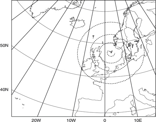
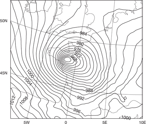
To further illustrate the flow-dependent character of the implicitly propagated background error covariance matrix, we have repeated the 4D-Var experiments, but now with insertion of the simulated surface pressure observation increment in a more dynamically stable area at 55°N 20°W, thus in the middle of a high pressure system at the time of observation (11 UTC), see Fig. 1. The resulting 4D-Var surface pressure increment at 11 UTC (Fig. 5) turns out to be quite different from the corresponding increment in the area of the storm development in Fig. 3. The similarity with the 3D-Var increments and the smaller amplitude of the increments at 11 UTC indicate a dominance of advective and diffusive processes in the propagation of the background error covariance matrix.

Fig. 5.  4D-Var surface pressure assimilation increments for 3 December 1999, 11 UTC, from a single surface pressure observation increment of −5 hPa at 55°N 20°W for 3 December 1999, 11 UTC. The data assimilation window is from 06 UTC until 12 UTC. The assumed standard deviation of the observation error is 0.5 hPa. The contour interval is 1 hPa.

These two examples of 4D-Var single simulated observation experiments provide evidence of the abilities of 4D-Var to take flow dependency into account. It needs to be stressed, however, that the flow dependency is limited to time scales corresponding to the length of the data assimilation window, since the background error covariance matrix is assumed static and flow independent at the start of the data assimilation window.

4. Model setup for HIRLAM 4D-Var tuning and validation experiments using real observations

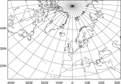
Parallel data assimilation and forecast experiments have been carried out in order to tune and to validate the performance of the HIRLAM 4D-Var. Some of these experiments were done for the reference HIRLAM (RCR) domain (Fig. 6) with 60 vertical levels and 582×448 horizontal grid points and with a horizontal grid resolution of 16 km in the non-linear model. Further experiments were carried out on the operational SMHI 22 km HIRLAM domain with 40 vertical levels. This domain includes 306×306 horizontal grid points and the domain has a reduced extension, mainly in the west, in comparison with the RCR domain.

Fig. 6.  The HIgh Resolution Limited Area Model RCR data assimilation and forecast domain.

Background error statistics for the experiments in this study were derived with the NMC-method (Parrish and Derber, 1992) and with input of forecast difference data (+36 h and +12 h forecasts valid at the same time) from the RCR domain and from all four seasons. This is certainly not the most optimal choice, since separate studies of moisture background error statistics, for example, have indicated a rather significant seasonal dependency of such background error statistics (Gustafsson et al., 2011).

The HIRLAM grid point forecast model applies a two-time level semi-Lagrangian semi-implicit integration scheme (Undén et al., 2002). The physical parameterisations include the Cuxart, Bougeault and Redelsperger (CBR) turbulence scheme (Cuxart et al., 2000), the Kain–Fritsch convection scheme (Kain, 2004), the Rasch–Kristjánsson cloud water scheme (Rasch and Kristjánsson, 1998), the simplified radiation scheme of Savijärvi (1990) and the ISBA surface and soil scheme (Noilhan and Mahfouf, 1996).

5. Tuning and validation of the weak digital filter constraint

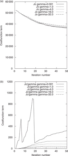
A problem with the weak digital filter constraint is the weight, given by the coefficient , to assign to the constraint. We will determine the value of through data assimilation experiments over the RCR model domain with a typical horizontal resolution of the first inner minimisation loop. The horizontal resolution of the non-linear forecast model is 16 km, while the horizontal resolution of the first inner minimisation loop is six times coarser (96 km). A total of 50 minimisation iterations were carried out with the conjugate gradient minimisation algorithm. Figure 7a shows the evolution with the iteration number of the observation constraint J _o , while Fig. 7b shows the evolution of , both for the following values of : 0.001, 1.0, 4.0, 16.0 and 32.0. J _o is a measure of the fit to the observations during the minimisation iterations, while is a measure of the magnitude of high-frequency oscillations during the TL model integrations. We can observe that a larger assigned value of the coefficient provides a direct response in the form of a stronger damping of high-frequency oscillations. We can also observe that for ≤4.0, the value of the observation constraint is only very weakly sensitive to . Thus by selecting =4.0 we will have a significant damping of high-frequency oscillations while, at the same time, the fit to observations will not be very much affected as compared to not applying the J _c constraint (this case is represented here by the J _o and J _c curves for =0.001).

Fig. 7.  The observation contribution J _o (a) and the normalised digital filter constraint contribution (b) to the total cost function as a function of the inner loop minimisation iteration number for different values of the weak digital filter constraint coefficient =0.001, 1.0, 4.0, 16.0 and 32.0. First outer loop iteration with 50 inner loop minimisation iterations for a horizontal increment resolution of 6× the non-linear model resolution. The RCR domain with 60 levels and 16 km horizontal resolution is applied in the non-linear model.

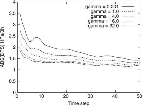
Just as important as the effect of reducing the amplitude of high-frequency oscillations in the TL model integrations of the minimisation itself is the need to damp high-frequency oscillations in non-linear forecast model runs issued from the analysis model states produced by the analysis. In our case, the model formulations differ (spectral TL model versus non-linear (NL) grid point model and different physical parameterisation schemes) as well as the horizontal model resolution (96 km for the TL model versus 16 km for the NL model). Taking these significant model differences into account, it is clear that the weak digital filter constraint is quite effective for reducing high-frequency oscillations in the high resolution NL model runs when the low-resolution assimilation increments are added to the high resolution background model state. This is illustrated in Fig. 8, which shows the area-averaged absolute value of the surface pressure tendency for every time step during the 5-h NL model integration until the mid-point of the last observation window of the data assimilation window. High-frequency oscillations as manifested in surface pressure tendencies are effectively damped by applying the weak digital filter constraint in the HIRLAM 4D-Var minimisation. Some high-frequency oscillations remain, most likely associated with non-linear interactions, with model physics, and with smaller scales not represented by the coarse resolution TL model, but these oscillations are damped quite quickly (≤1 h) in the NL model integrations.

Fig. 8.  Horizontal average of the absolute value of the surface pressure tendency (in hPa/3 h) for every time-step, with a time step length of 6 minutes, during the non-linear model integration over 5 h from initial data based on HIgh Resolution Limited Area Model 4D-Var, including a weak digital filter constraint with different values of the weak digital filter constraint coefficient =0.001, 1.0, 4.0, 16.0 and 32.0. One outer loop iteration with 50 inner loop minimisation iterations for a horizontal increment resolution of 6× the non-linear model resolution and the RCR domain with 60 levels and 16 km horizontal resolution in the non-linear model are applied.

For the RCR model domain with 60 levels and with a 16 km horizontal resolution, we have made the choice to use =4.0 for inner loop minimisation iterations with a horizontal increment resolution six times coarser than the original non-linear model resolution. For the same non-linear model configuration, it turned out that a reasonable value of could be obtained for other horizontal resolutions of the inner minimisation loops simply by taking the squared number of increment components into account. For example, for a horizontal increment resolution three times coarser than the original non-linear model resolution, a value of =0.25 = 4.0/(2 * 2)² turned out to be efficient, with =4.0 being the value optimised for a horizontal increment resolution six times coarser than the non-linear model resolution. Note that the horizontal integration weights for the total energy norm are set to be constant (=1).

6. Tuning and validation of the multi-incremental minimisation

The multi-incremental design of the HIRLAM 4D-Var minimisation provides flexibility. The number of outer loop iterations can be varied, and the horizontal resolution of the assimilation increment as well as the choice of simplified physics for each iteration in the outer loop may also be varied. The time step for the TL and AD models needs to be specified such that numerical instability is avoided. The fraction of the total wind increment to be determined in a particular outer loop iteration sets the requirement on maximum time step for stability (see discussion in Subsection 2.4.1). Therefore, it is an advantage for computational efficiency if a larger fraction of the assimilation increment can be calculated within outer loop iterations with coarser resolution of the assimilation increment. Finally, there is also some flexibility with regard to the application of observation quality control within the 4D-Var assimilation. Variational quality control is switched on over a specified range of inner loop minimisation iterations in one of several outer loop minimisation iterations. With 3D-Var or with 4D-Var with one outer loop iteration, it turned out to be beneficial to switch on VarQC during an early part of the inner loop minimisation iterations, to reject all observations not passing the VarQC and to solve a fully quadratic minimisation problem for the remaining inner loop iterations. On the other hand, with several outer loop iterations, it may be argued that VarQC should be applied at highest possible resolution and with an improved model state available to support the quality control decisions, normally during the last outer loop iteration.

We have carried out some sensitivity experiments in order to understand better and to be able to specify in more detail the minimisation design. These experiments were carried out for the RCR domain with 60 vertical levels and with a horizontal resolution of 16 km of the non-linear model. As a reference we applied a single relatively high resolution (48 km) outer loop minimisation iteration with a sufficient number of iterations (100) in the inner loop minimisation. To be comparable to the multiple outer loop minimisation tests, see below, VarQC was applied between iteration 65 and 75. Secondly, we carried out a minimisation with two iterations in the outer loop, both with 50 iterations and with the same horizontal resolution (48 km) in the inner loop minimisations. Finally, we carried out two experiments, again with two outer loop iterations but with a coarser resolution (96 km) in first outer loop iteration. One experiment had 60 inner loop iterations in the first outer loop iteration and 40 inner loop iterations in the second outer loop iteration. For the second experiment, we reduced the number of inner loop iterations to 30 in the first outer loop iteration and increased the number of inner loop iterations to 70 in the second outer loop iteration. For the experiments with two outer loop iterations, we placed the VarQC between the same inner loop iteration numbers as in the single outer loop experiment in order to have comparable results.

The performance of the minimisation with the different strategies is illustrated for the variation of the observation constraint (J _o ) as a function of the iteration number in Fig. 9a and for the corresponding background error constraint (J _b ) in Fig. 9b. Firstly, we may notice the drop in J _o when the observation error non-Gaussian PDF of the VarQC is switched on in iteration 65 and the further drop when all rejected observations are removed from cost function contributions in iteration 75. Secondly, we can notice that the convergence towards fit to the observations, measured by J _o , is faster with a higher resolution of the assimilation increments from the start of the minimisation. Concerning the comparison between a minimisation with a single outer loop (100 inner loop iterations) and two outer loop iterations (50 + 50 iterations) at 48 km increment resolution, we may notice a slight retardation of the convergence towards observations at the start of the second outer loop due to a minimisation restart. More importantly, we see a better fit to observations in the two outer loop cases as compared to the single outer loop case, by the end of the minimisation. This is most likely due to a benefit of the relinearisations in the second outer loop.

Fig. 9.  The observation error constraint contribution J _o (a) and the background error constraint contribution J _b (b) to the total cost function as a function of the total inner loop minimisation iteration number for four different minimisation strategies: (1) one outer loop minimisation with a 48 km horizontal resolution of the assimilation increment and with 100 inner loop iterations; (2) two outer loop iterations, both with 50 iterations in the inner loops and with 48 km resolution of the increments; (3) and (4) two experiments with two outer loop iterations, both with 96 km resolution in the first outer loop and with 48 km in the second outer loop, one experiment with 30 inner loop iterations in the first outer loop and with 70 iterations in the second outer loop. Another experiment has 60 iterations in the first outer loop and 40 iterations in the second outer loop. The RCR domain with 60 levels and 16 km horizontal resolution in the non-linear model is applied.

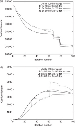
With regard to the experiments with a coarser resolution in the first outer loop than in the second outer loop (96 vs. 48 km), we see a clear retardation of the convergence towards fit to observations (J _o ) in the experiment with 60 inner loop iterations in the first outer loop. This indicates that there is very little to gain with these coarse resolution increments beyond iteration 40, and further iterations are meaningless since they will only provide an over-fit to the observations of the larger scale increments. This effect is clearly seen also in the behaviour of the J _b as a function of iteration number (Fig. 9a). After 60 iterations with a coarse resolution increment, we can first see a jump in J _b , due to the renormalisation of the horizontal spectral densities between the outer loop iterations, and then a drop in J _b throughout the second outer loop minimisation that could partly be explained by redistribution of increment variability from larger scales to the smaller horizontal scales available in the second outer loop at finer resolution. The same effect, but less pronounced, can be seen in the J _b -curve for the experiment with 30 and 70 inner loop iterations, respectively. One may say that with fewer inner loop iterations in the first outer loop iteration at coarser resolution, there is less need for a redistribution of increment variability from larger to smaller scales in the second outer loop iteration.

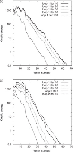
In order to illustrate more directly the spectral characteristics of the assimilation increments during the minimisation, we have calculated the kinetic energy spectra of the assimilation increments. Figure 10a shows the kinetic energy spectra at model level 30 (around 500 hPa) after 10, 20, 30, 60 and 100 inner loop iterations of the single outer loop minimisation at 48 km horizontal resolution. It is quite clear that mainly large horizontal scales are established during the first inner loop iterations of the minimisation and that the horizontal scales of the increment gradually becomes smaller and smaller with the inner loop iteration number. From this we can conclude that it may be sufficient to run a limited number of inner loop iterations in the first outer loop iteration at coarse resolution, in case the intention is to establish the large-scale part of the assimilation increment. This is confirmed by the kinetic energy spectra at the corresponding inner loop iterations of the experiment with 60 inner loop iterations at 96 km in the first outer loop and with 40 iterations at 48 km in the second outer loop iteration (Fig. 10b). Thus, if we take as many as 60 iterations in the first outer loop at a coarse resolution, we may notice that the change in the kinetic energy spectrum over the 40 iterations of the second outer loop is mainly a redistribution of energy from larger scales to smaller scales. An experimental design of multi-incremental minimisation strategies for 4D-Var, with results similar to those presented here, has been reported by Lawless and Nichols (2006).

Fig. 10.  Kinetic energy spectrum at model level 30 (around 500 hPa) for the assimilation increments. (a) After 10, 20, 30, 50 and 100 inner loop iterations of a 4D-Var minimisation with a single outer loop iteration with a 48 km horizontal resolution of the increments. (b) Same as in (a) but for the experiment with two outer loop iterations, with 60 iterations at 96 km resolution in the first outer loop and with 40 iterations at 48 km in the second. The assimilation was carried out with the HIgh Resolution Limited Area Model 4D-Var for the RCR domain with 60 levels and 16 km horizontal resolution in the non-linear model.

In order to investigate the impact of different minimisation strategies on the forecast quality, a few minimisation strategies were applied in a 1-month-long data assimilation and forecast experiment over the SMHI domain with a 22 km horizontal resolution and with 40 vertical levels. The data period of June 2005 was selected, thus a summer period with smaller spatial scales of importance, that could enhance the sensitivity to the minimisation. Figure 11 shows the BIAS (mean error) and Root Mean Square Error (RMSE) verification scores for MSLP, as verified against SYNOP observations, for three of these experiments: (1) a single outer loop at 44 km increment resolution with 100 inner loop iterations; (2) a single outer loop at 66 km increment resolution with 100 inner loop iterations; (3) two outer loop iterations at 66 and 44 km resolution, respectively, and with 50 inner loop iterations each. We show the verification scores for a Scandinavian domain, since the impact of the minimisation scheme turned out to be strongest in the centre of the model domain.

Fig. 11.  BIAS (mean error, thin lines) and root mean square error (RMSE, thick lines) mean sea level pressure (MSLP) verification scores for June 2005 as a function of forecast length. Verification against surface observations over a Scandinavian domain. Experiment 4DVAR1 (full lines): 4D-Var with one outer loop iteration at 66 km resolution, experiment 4djun05D (dashed lines): 4DVAR with one outer loop iteration at 44 km resolution and experiment 4DVAR2 (dotted lines): 4DVAR with two outer loop iterations at 66 km and 44 km resolution, respectively.

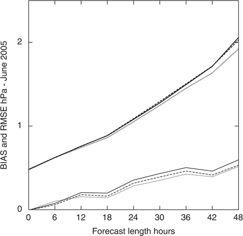
From the results in Fig. 11, we can see that the RMSE MSLP forecast verification scores for this month of experimentation do not depend so strongly on the resolution, whether 66 or 44 km, of the assimilation increment in a single outer loop iteration minimisation. But more importantly, we can see that with two iterations in the outer loop minimisation we get reduced RMSE verification scores. The significance of the time-averaged RMSE verification score differences in Fig. 11 was also checked by a student's t-test (for details on the significance test see below). It turned out that the RMS score differences between the experiments with a single and with two outer minimisation loops were significant at the 90% level for forecasts longer than +6 h, while the forecast score differences for the experiments with different inner loop resolutions were not significantly different. For the same three experiments, BIAS and RMSE verification scores for vertical temperature and wind profile forecasts (not shown), as verified against radiosonde data, indicated a similar pattern but with less significant differences between the three experiments.

To summarise, the application of the multi-incremental minimisation turns out to be an efficient tool for reducing the computational cost of the HIRLAM 4D-Var as well as for improving the model initial state through the relinearisations of the forecast model and the observation operators carried out between the outer loop iterations.

7. Comparisons between HIRLAM 4D-Var and 3D-Var

In order to validate the performance of the HIRLAM 4D-Var and compare it with the performance of 3D-Var, parallel data assimilation and forecast experiments have been carried out over the 4 months: April 2004, January 2005, June 2005 and January 2007. The performance of 4D-Var with two different numbers of outer loop iterations was compared as well. These experiments were done for the operational SMHI domain with 22 km horizontal resolution and with 40 vertical levels. To illustrate the effects of HIRLAM 4D-Var for individual cases, parallel data assimilation and forecast experiments were carried out also for the stormy month of December 1999 on the larger RCR horizontal domain (Fig. 6), with a 16 km horizontal resolution and with 60 vertical levels.

7.1. The data assimilation experiments using the operational SMHI domain

The following three versions of data assimilation were compared:

• 3DVar: HIRLAM 3D-Var with the FGAT of the observations, with a 6-h data assimilation window in a 6-h data assimilation cycle and with an incremental DFI. The assimilation increments were calculated in spectral space with a shortest resolved wavelength of 66 km.

• 4DVar1: 4D-Var with one iteration in the outer loop minimisation, with a 6-h data assimilation window and with the observations collected in six observation time windows of ±30 minutes around each full hour. The shortest resolved wavelength of the assimilation increments was 132 km (66 km grid point resolution) and the time step of the TL and AD models was 30 minutes. The maximum number of iterations in the inner loop minimisation was 70. No explicit initialisation was applied, relying solely on the weak digital filter constraint during the 4D-Var minimisation.

• 4DVar2: 4D-Var with two iterations in the outer loop minimisation, with a 6-h data assimilation window and with the observations collected in six observation time windows of ±30 minutes around each full hour. The first outer loop iteration was applied with a shortest resolved wavelength of 132 km and with maximum 40 iterations in the inner loop minimisation. The second outer loop iteration was applied with a shortest resolved wavelength of 88 km and with maximum 30 iterations in the inner loop minimisation. The time step of the TL and AD model integrations was 30 minutes in both outer loop minimisation iterations. No explicit initialisation was applied, relying solely on the weak digital filter constraint of the 4D-Var minimisation.

Variational quality control was applied in all three experiments. Variational quality control was switched on between inner loop iterations 15 and 25 of experiments 3DVar and 4DVar1 and similarly applied only during the second outer loop minimisation iteration of experiment 4DVar2. Once VarQC was switched off, observations considered as rejected by the VarQC algorithm were no longer used.

The following types of observations were utilised for the data assimilation experiments: temperature, wind and specific humidity profiles from TEMP reports; wind profiles from PILOT reports; surface pressure measurements from SYNOP, SHIP and DRIBU reports; wind and temperature measurements from aircraft reports (AIREP and AMDAR) and, finally, AMSU-A satellite radiance measurements over seawater and sea ice surfaces only. A bias correction, following Harris and Kelly (2001), was applied to the AMSU-A radiance measurements.

Operational ECMWF global forecasts were used for the lateral boundary conditions of the experiments, with a shift 6 h backward in initial time for the lateral boundary conditions as compared with the initial time of the HIRLAM experiment.

7.2. Observation selection

In addition to the algorithmic differences, the operational application of HIRLAM 3D-Var and 4D-Var also differ with respect to the selection of observations to influence the assimilation. The 3D-Var applies a 3-dimensional data selection, including data thinning, for the whole 6-h observation window, while the 4D-Var applies the same type of data selection to each of the hourly observation windows. Table 1 presents the number of observed values that enter into the 3D-Var and 4D-Var minimisations, after screening quality control and data thinning, for two typical data assimilation cycles, one at 06 UTC and one at 12 UTC.

Table 1. Numbers of Active Observed Values that Enter the 3D-Var and 4D-Var Minimisations for 12 January 2007 06 UTC (a) and 12 UTC (b)

	3D-Var	4D-Var
	06	03	04	05	06	07	08
(a) Type and variable	UTC	UTC	UTC	UTC	UTC	UTC	UTC	Total
TEMP u/v	785	21	0	0	712	35	50	818
TEMP T	735	20	0	0	624	67	62	773
TEMP q	689	20	0	0	578	62	62	722
PILOT u/v	114	0	0	0	114	0	0	114
SYNOP p s	2106	1900	862	860	2041	872	864	7399
SHIP p s	167	85	65	64	113	63	67	457
DRIBU p s	57	50	54	54	51	48	38	295
Airep u/v	1928	143	273	288	422	412	314	1852
AIREP T	1950	142	273	290	438	414	316	1874
AMSU-A rad.	21230	5680	0	9190	90	8760	0	23720
	3D-Var	4D-Var
	12	09	10	11	12	13	14
(b) Type and variable	UTC	UTC	UTC	UTC	UTC	UTC	UTC	Total
TEMP u/v	6427	0	0	181	6255	537	0	6973
TEMP T	5381	0	0	109	5266	547	0	5922
TEMP q	4499	0	0	109	4384	19	0	4512
PILOT u/v	33	0	0	0	33	0	0	33
SYNOP p s	2114	1999	874	881	2086	872	861	7573
SHIP p s	160	86	68	68	112	31	30	395
DRIBU p s	59	44	53	50	52	47	17	263
Airep u/v	2952	223	497	608	653	513	420	2914
AIREP T	2968	228	508	612	655	513	419	2935
AMSU-A rad.	7890	0	1230	1080	2370	3490	0	8170

We may notice that the main effect of the 4D-Var data selection is the increased number of selected surface pressure observations as compared to the 3D-Var data selection. The reason is that the current HIRLAM 3D-Var data selection only extracts one report from the same observation station and the same observation window. Since 3D-Var neglects the time variation of the assimilation increment over the assimilation window, it is considered appropriate to select only the report closest in time to the nominal assimilation time in this case. With the 4D-Var data selection designed for a time-variable assimilation increment, we will thus have a chance to utilise the dynamical information inherent in a time series of surface pressure measurement. On the other hand, in case of a significant time correlation of errors of surface observations from the same station, there is an obvious risk with the present 4D-Var data selection algorithm to over-fit the influence of such observations.

Note that the efficient number of AMSU-A radiance measurements that were utilised during the minimisation should be reduced by a factor ≥ 0.6 from the figures in Table 1 since radiance channels 1–4 (out of 10) are given very small weights by applying very large observation error standard deviations because these satellite radiance measurements are strongly influenced by surface conditions.

7.3. Forecast verification scores

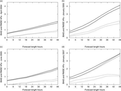
Forecasts up to +48 h were produced every 6 h from the 4 months of data assimilation. These forecasts were verified against SYNOP and TEMP observations. Time-averaged verification scores for MSLP forecasts, in the form of BIAS (mean error) and RMSE, as functions of forecast length and for a Scandinavian area in the centre of the full forecast domain, are presented in Fig. 12. The reduction in RMSE verification scores for surface pressure by the 4D-Var in comparison with 3D-Var is clearly seen for all 4 months of experimentation. We can also notice a (smaller) reduction in the RMSE verification scores for the experiment with two 4D-Var outer loop minimisation iterations in comparison with only one outer loop minimisation iteration. The significancy of the RMSE verification score differences in Fig. 12 was checked by a student's t-test. On the 90% significancy level, the RMSE scores for the 4D-Var-based forecasts turned out to be significantly smaller than the RMSE scores for the 3D-Var-based forecasts for all forecast lengths and for all 4 months, while the RMSE scores for forecasts based on 4D-Var two outer loop iterations were significantly smaller than the scores with one outer loop for June 2005 and January 2007 only. The BIAS verification scores indicate a rather systematic positive valued bias for all 4 months of experimentation. This bias is most likely linked to the cold tropospheric bias that the HIRLAM forecast model used for the present experimentation was affected by.

Fig. 12.  BIAS (Mean error, thin lines) and root mean square error (RMSE, thick lines) mean sea level pressure (MSLP) forecast verification scores for a Scandinavian domain as a function of forecast length. Time averaged scores for April 2004 (a), January 2005 (b), June 2005 (c) and January 2007 (d). 3D-Var (full line), 4D-Var with one outer loop iteration (dashed line) and 4D-Var with two outer loop iterations (dotted lines).

Mean sea level pressure verification scores for a complete European domain also indicate a positive impact of 4D-Var in comparison with 3D-Var for the 4 months of comparison. Although the magnitudes of the forecast score differences are smaller over the European domain than over the Scandinavian domain, since forecasts for verification stations closer to the lateral boundaries will be much faster influenced by the lateral boundary conditions, the time averages of the differences are statistically significant. We show normalised mean RMSE forecast verification score differences between 3D-Var and 4D-Var (with one outer loop iteration) for MSLP and for all 4 months of experimentation over a European domain as a function of forecast length in Fig. 13. Vertical bars represent significance at the 90% level based on a student's t-test. To determine whether the differences in results between the two experiments A and B were statistically significant, we performed a student's t-test for the normalised mean difference δ _AB in forecast-minus-observation RMSE scores.9

Fig. 13.  Normalised mean root mean square error (RMSE) forecast verification score differences (green curves) between 3D-Var and 4D-Var (with one outer loop iteration) for mean sea level pressure (MSLP) over a European domain as a function of forecast length. Time-averaged scores for April 2004 (a), January 2005 (b), June 2005 (c) and January 2007 (d). Vertical red bars represent significance at the 90% level.

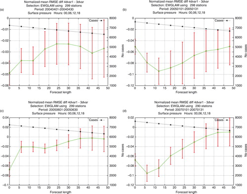
We assumed that the normalised RMSE score differences have a Gaussian distribution and a serial correlation in time. The serial correlation was assumed to be lag-one autoregressive. The autocorrelation ρ of the time series of the normalised RMSE score differences of these parameters was computed and used to correct the sample size and subsequently modify the variance accordingly.

BIAS and RMSE forecast verification scores for upper air variables as verified against radiosonde observations (not shown) indicated a neutral or a small positive impact of the 4D-Var experiments over the 3D-Var experiments for all 4 months of experimentation. The positive impact in RMSE verification scores for 4D-Var as compared to 3D-Var was largest at upper air jet levels (around 300 hPa), and this, together with the positive impact for MSLP forecasts, is an indication that the improvement provided by 4D-Var mainly concerns the handling of baroclinic, synoptic scale, disturbances in the data assimilation process. The cold lower troposphere temperature bias was quite obvious in the temperature verification scores.

7.4. A case study – the stormy month of December 1999

During December 1999, three major storms hit Europe with devastating effects on human life and material resources. In the evening of 3 December 1999, a very intensive mesoscale low pressure system hit Jutland in western Denmark (see Fig. 14), on 26 December another storm hit Northern France and Germany (not shown), and 2 d later another mesoscale storm hit western and central France (see Fig. 15).

Fig. 14.  HIgh Resolution Limited Area Model 4D-Var mean sea level pressure (MSLP) analysis for 3 December 1999, 18UTC. The contour interval is 2 hPa.

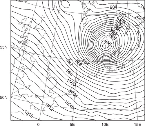
Fig. 15.  HIgh Resolution Limited Area Model 4D-Var mean sea level pressure analysis for 27 December 1999, 18 UTC. The contour interval is 2 hPa.

Since forecasting of major storm developments is strongly sensitive to the baroclinicity of the initial states for the forecast model integrations, and as we have already demonstrated (see Section 3) that the HIRLAM 4D-Var provides a quite different flow-dependent influence of individual observations compared to HIRLAM 3D-Var in such storm situations, we decided to rerun data assimilation and forecasts for the whole month of December 1999 with both assimilation methods. The experiments were carried out on the larger RCR domain, with a model grid resolution of 16 km and with 60 vertical levels. Two outer loop iterations were applied in the 4D-Var minimisation. The lateral boundary conditions for these December 1999 experiments were extracted from the ECMWF ERA-40 reanalysis archives. Since only forecasts up to +6 h were available from ERA-40 at 06 UTC and 18 UTC, it was not possible to apply the FGAT option in the HIRLAM 3D-Var assimilation runs.

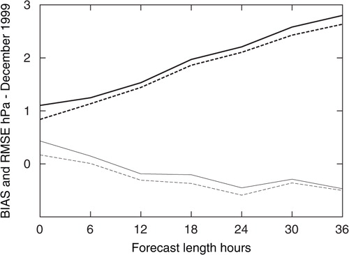
Time-averaged MSLP forecast verification scores for December 1999 in the form of BIAS and RMSE, as functions of forecast length for a European domain, are presented in Fig. 16. The reduction in RMSE verification scores for MSLP by the 4D-Var in comparison with 3D-Var is clearly seen also for the December 1999 experiment. One particularity with these verification scores for December 1999 is the large difference in the RMS scores (and also the large positive BIAS for the 3D-Var scores) at +0 h, for the deviations between the analyses and the observations. By examining time series of forecast verification scores as well as forecast verification scores for subdomains over Denmark and France (not shown), it was found that these large differences at initial time were caused by numerous rejections of correct observations in the case of 3D-Var data assimilation, in particular during the intensive mesoscale storm events, while the 4D-Var data assimilation was more successful in this respect.

Fig. 16.  BIAS (mean error, thin lines) and root mean square error (RMSE, thick lines) mean sea level pressure (MSLP) forecast verification scores for a European domain as a function of forecast length. Time averaged scores for December 1999. 3D-Var (full lines) and 4D-Var (dashed lines).

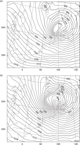
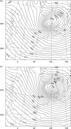
The short range forecasts of the three major storms in December 1999 were all improved by using HIRLAM 4D-Var for the data assimilation in comparison with HIRLAM 3D-Var. We present a few examples. The +30-h MSLP forecasts valid at 3 December 1999 18 UTC are shown in Fig. 17 with the forecast based on 3D-Var initial data in panel (a) and with the forecast based on 4D-Var initial data in the panel (b). The forecast based on 4D-Var has a much improved structure and intensity of the low pressure development with 959 hPa in the centre of the low, as compared with 971 hPa in the 3D-Var-based forecast and with the verification analysis (see Fig. 14) with 953 hPa in the centre of the low.

Fig. 17.  +30 h mean sea level pressure (MSLP) forecasts valid at 3 December 1999, 18 UTC, based on 3D-Var (a) and 4D-Var (b) initial data from 2 December 1999, 12 UTC. The contour interval is 2 hPa.

Comparing the +18 h-MSLP forecasts valid at the same time (Fig. 18) we may notice that both the 3D-Var- and the 4D-Var-based forecasts have improved as compared to the forecasts based on 12 h earlier initial data. The 4D-Var-based forecast is still significantly better than the 3D-Var-based forecast, with respect to the position of the low pressure system as well as with respect to the intensity of the low pressure development (957 hPa in the 4D-Var case and 963 hPa in the 3D-Var case). It should be added that the 3D-Var-based verification analysis of the MSLP (not shown) is very similar to the 4D-Var-based verification analysis as shown in Fig. 14.

Fig. 18.  +18 h mean sea level pressure (MSLP) forecasts valid at 3 December 1999, 18 UTC, based on 3D-Var (a) and 4D-Var (b) initial data from 3 December 1999, 00 UTC. The contour interval is 2 hPa.

The question arises concerning the origin of the forecast improvements caused by the 4D-Var initial data as compared to the 3D-Var initial data for the particular case of the storm development in the evening of the 3 December 1999. Since the storm development was generally quite predictable, it was necessary to follow analysis and forecast differences upstream and backwards in time for several days. The assimilation increments were quite small, generally leading to quite small forecast improvements, both with 3D-Var and with 4D-Var, for each assimilation cycle. Thus, it was not possible to identify any specific treatment of any observation that caused the major improvements by the 4D-Var assimilation. What became obvious, however, were the significant differences between the structures of the 3D-Var and 4D-Var assimilation increments, with 4D-Var showing distinct flow-dependent increment structures. We demonstrate this here by showing the 3D-Var and 4D-Var surface pressure assimilation increments over the North Sea for two assimilation cycles, 3 December 1999 06 UTC in Fig. 19 and 3 December 1999 12 UTC in Fig. 20, both during the most intensive mesoscale storm development.

Fig. 19.  Surface pressure assimilation increments for 3 December 1999, 06 UTC, with 3D-Var (a) and with 4D-Var (b). The contour interval is 1 hPa.

Fig. 20.  Surface pressure assimilation increments for 3 December 1999, 12UTC, with 3D-Var (a) and with 4D-Var (b). The contour interval is 1 hPa.

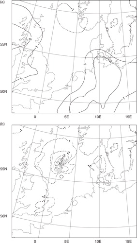
The most obvious differences between the 3D-Var and 4D-Var assimilation increments in Figs. 19 and 20 are the differences in horizontal scale. The horizontal scales of the 3D-Var assimilation increments reflect the large-scale (and smooth) synoptic scale structures of the static 3D-Var assimilation structure functions, describing the long-term average structures of background errors, while the 4D-Var assimilation increments are dominated by mesoscale structures reflecting the current instabilities of the flow, that is, the assimilation structures are strongly flow-dependent. There are clear similarities between the real 4D-Var assimilation increments valid at 3 December 1999 12 UTC in Fig. 20 and the 4D-Var assimilation increments from the single simulated observation experiment in Fig. 3.

With regard to the 3D-Var assimilation increments from two consecutive assimilation cycles, there was a rather large-scale negative surface pressure increment at 3 December 1999 06 UTC, when the mesoscale low pressure system was positioned over land (the British Isles) with many SYNOP observation stations, while there were large-scale positive (thus compensating) surface pressure increments 6 h later, when the mesoscale low pressure system was positioned over the less observation dense North Sea. More generally, 3D-Var favours extrapolation from data dense areas to data sparse areas with large-scale static 3D-Var structure functions. In cases when the real forecast errors have much smaller scales, such as in this case of a mesoscale storm development, this will result in assimilation increments that are too large-scale, and this can be seen as a detrimental aliasing effect.

The mesoscale storm, also known as the ‘Second French Christmas Storm’, that hit the French Atlantic coast in the evening of 27 December 1999 has been studied by several modelling groups, and it has been shown to be quite unpredictable and sensitive to even small changes in the use of observations, both in the data assimilation details and in the forecast model. This is also the case with the present 3D-Var and 4D-Var data assimilation experiments. With the 3D-Var data assimilation, the intensity of the mesoscale low was only captured when the mesoscale low had already moved in over French territory with a denser network of SYNOP stations. Due to the poor background model state, and due to the large-scale static 3D-Var assimilation structure functions applied in the VarQC, it takes the 3D-Var several assimilation cycles to capture the low pressure development, since most of the important observations are simply rejected. The +6 h-MSLP forecast from the 3D-Var data assimilation cycle, valid for 27 December 1999 18 UTC, is presented in Fig. 21a, to be compared with verification analysis in Fig. 15 and the corresponding 4D-Var-based +6 h forecast in Fig. 21b. Note that the 4D-Var-based +6 h forecast is the background state for the verification analysis, but what is important is that the 4D-Var analysis (as well as the analysis background state) agrees with the observations and avoids the rejection of all important observations as in the 3D-Var assimilation cycle. This poor treatment of the observations in the 3D-Var assimilation cycle is even seen in the average verification scores for the whole month of December 1999 over the European domain (Fig. 16). One may speculate whether FGAT and a data selection similar to the 4D-Var data selection would have improved the 3D-Var performance. On the one hand, the VarQC data rejection algorithm would certainly have had a better chance to accept more observations due to the support from a time series of observed values in each station. On the other hand, the intensity of the storm development was caught by 4D-Var already over the data-sparse sea areas, where data selection should be less of a problem and where implicit flow-dependent structure functions are likely to be more important.

Fig. 21.  +6 h mean sea level pressure (MSLP) forecasts valid at 27 December 1999, 18 UTC, based on 3D-Var (a) and 4D-Var (b) initial data at 27 December 1999, 12 UTC. The contour interval is 2 hPa.

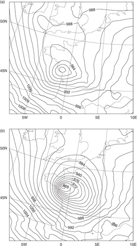
7.5. Summary of comparisons between HIRLAM 4D-Var and HIRLAM 3D-Var

Data assimilation and forecast experiments have been carried out for five data periods of 1 month each. These experiments indicate the clear positive impact of HIRLAM 4D-Var as compared to 3D-Var as measured by forecast verification scores. HIRLAM 4D-Var provides the possibility of using more observations, for example, several observations from the same station within the 6-h data assimilation windows, as well as the advantages of applying implicit flow-dependent assimilation structure functions within these assimilation windows. The experiments carried out for the stormy month of December 1999 indicate that the implicit flow-dependent structure functions of HIRLAM 4D-Var provide a substantial part of this positive impact, directly by producing more realistic data assimilation increments and VarQC decisions, and indirectly through an improvement of the whole data assimilation cycling.

8. Remarks on the HIRLAM 4D-Var code

The HIRLAM 4D-Var computer code is based on the semi-Lagrangian spectral HIRLAM code (Gustafsson and McDonald, 1996). The code is written in Fortran 90 and with two levels of parallelisation, MPI for communication between distributed memory computer nodes and OpenMP for parallelisation between computer processors sharing memory within the same computing node. The parallelisation for the non-linear, TL and AD spectral models has been described by Gustafsson (1999). Grid point space calculations are based on a 1-dimensional area decomposition in the y-direction only for the upper level of parallelisation, which sets a limit on the maximum number of computer nodes for which the assimilation code can be applied. Spectral calculations, for example in the solving of the semi-implicit equations, are based on a two-dimensional area decomposition. The transposition of data between the grid point space and the spectral space area decompositions, essentially carried out within the spectral (FFT) transforms, is done by message passing (MPI commands). The parallelisation of the observation handling was suggested by Rantakokko (1997). All horizontal interpolations from grid point space to the positions of the observations are carried out on the processors where the grid point information resides in accordance with model area decomposition, while the remaining computational work of the observation operators is shared equally between the computational nodes by letting each computational node take care of the same number of observations of each observation type. An efficient handling of the area extension zone, needed in order to provide bi-periodic variations required by the spectral transforms, is a critical issue in the parallelisation of the HIRLAM 4D-Var, since the extension zone has to be wide enough to let horizontal correlations approach zero over the distance of the width of the extension zone. This is achieved by doing the model domain decomposition and all grid point calculations over the real (unextended) model domain only. In this way only the spectral transforms and the spectral space calculations are affected by the extension zone with only a minor dependence of the total calculation time on the width of the extension zone.

We have included in Table 2 a coarse profiling of the computation time for HIRLAM 4D-Var on the RCR domain (16 km resolution and 60 vertical levels) for an IBM parallel computer utilising 32 processors on a single computing node. Calculation times include two outer loop iterations, the first with 30 inner loop iterations at 96 km horizontal resolution and the second with 40 inner loop iterations at 48 km horizontal resolution, as well as the non-linear model trajectory and forecast calculations. The first thing to be noticed is the relatively long time spent in reading and writing the grid point fields, although this process has also been made partially parallel. The second thing to be noticed is the dominance of the TL and AD model calculations during the minimisations. A large fraction of the TL and AD model calculations is devoted to the semi-Lagrangian (SL) part of the calculations, and out of the SL calculation time a large fraction of the time (75%) is spent on communication between the processors. Due to the relatively long time steps applied in the HIRLAM 4D-Var, information from neighbouring processors is needed over the so-called ‘halo zones’ with a width of 6–8 grid lengths. Similarly, the calculation time for the spectral transforms includes a large fraction of inter-processor communications (memory transpositions). We may finally note that the total cost for HIRLAM 4D-Var with the described multi-incremental minimisation is of the same order as that for a 48-h non-linear model forecast.

Table 2. Example of Computation Times in Seconds on an IBM Computer with 32 Processors for Different parts of HIRLAM 4D-Var

(a)NL 5 h trajectory for outer loop 1: 120 s
Minimisation outer loop 1: 107 s	TL and AD models: 83 s	SL calc.: 30 s
		FFTs: 24 s
		SI calc.: 9 s
		Physics: 20 s
	J b : 3 s
	J o : 10 s
Read and write fields in outer loop 1: 63 s
Prepare observations in outer loop 1: 19 s
(b)NL 5 h trajectory for outer loop 2: 120 s
Minimisation outer loop 2: 285 s	TL and AD models: 241 s	SL calc.: 80 s
		FFTs: 80 s
		SI calc.: 25 s
		Physics: 56 s
	J b : 12 s
	J o : 18 s
Read and write fields in outer loop 2: 191 s
Prepare observations in outer loop 2: 17 s
NL 48 h forecast: 850 s

(a) 30 inner loop iterations at 96 km increment resolution; (b) 40 inner loop iterations at 48 km increment resolution, both with 60 vertical levels. The non-linear model domain is the RCR with a 16 km horizontal resolution.

9. Concluding remarks

We have here provided a rather detailed description of the HIRLAM 4D-Var, including the multi-incremental minimisation, the TL and AD models based on the spectral, semi-Lagrangian and semi-implicit version of the HIRLAM forecast model, the comprehensive observation handling system and the weak digital filter constraint.

The ability of the HIRLAM 4D-Var to provide implicit flow-dependent assimilation structure functions, giving a flow-dependent influence of observations within the assimilation window, was demonstrated for a mesoscale storm development over the North Sea on the 3 December 1999 (‘the Danish storm’). The flow-dependent structure functions provided in the centre of the storm development were contrasted to structure functions in areas of weaker dynamical instabilities as well as to flow-independent 3D-Var structure functions.

For a good performance of the weak digital filter constraint, it is necessary to provide well-tuned values of the weighting coefficient in front of the constraint. With such well-tuned values, high-frequency oscillations are efficiently damped during the TL model integrations and also, which cannot be taken for granted, during the non-linear model integrations initialised with HIRLAM 4D-Var initial state data. It is demonstrated that no explicit initialisation is needed when the weak digital filter constraint is applied during the HIRLAM 4D-Var minimisation.

The multi-incremental minimisation of the HIRLAM 4D-Var provides flexibility, but the design of the multi-incremental scheme necessitates some care. On the one hand, it is shown that several outer loop iterations provide improved initial conditions, as measured by improved forecast verification scores, due to relinearisation of the non-linear forecast model and the non-linear observation operators. On the other hand, coarse resolution (and computationally cheap) outer loop iterations cannot be applied with too many inner loop iterations as it will just be a waste of computational resources since such coarse resolution outer loops will project the observation increments onto too large spatial scales that have to be adjusted later on during more high resolution outer loop iterations.

For the operational application of the HIRLAM 4D-Var, it has been possible to design a multi-incremental minimisation scheme such that the total cost of the HIRLAM 4D-Var is approximately equal to the cost of a +48 h forecast. Such multi-incremental versions of the HIRLAM 4D-Var have been operationally implemented at the Swedish, Finnish and Irish weather services.

The HIRLAM 4D-Var has been proven to consistently out-perform the HIRLAM 3D-Var over 5 months of data assimilation and forecast experiments, as proven by forecast verification scores. Identified cases of significant improvement include mainly strong mesoscale storm developments, pointing to the abilities of 4D-Var to improve the initial baroclinicity of importance for such storm developments.

Future activities with regard to 4D-Var and data assimilation in general include further development of the hybrid variational ensemble data assimilation for HIRLAM allowing for flow-dependent assimilation structure functions also at the start of the assimilation window and development of 4D-Var for the mesoscale HARMONIE forecasting system built on the ECMWF IFS (Integrated Forecast System). It is also crucial for the forecasting performance to improve data assimilation aspects of the coupling to the host model. The HIRLAM forecasting system is generally applied with forecast lateral boundary conditions from an earlier global model run than the actual HIRLAM forecast run. Any limited area data assimilation has difficulties in properly assimilating the larger scales, and for this reason, it is not sufficient to refresh only the lateral boundaries but it is also necessary to adapt the large scales in the interior of the LAM domain from the information given by a new global forecast run. Furthermore, for a LAM 4D-Var data assimilation, it is also necessary to control the lateral boundary conditions in order to utilise more efficiently observations in the vicinity of these lateral boundaries.

10. Acknowledgements

We thank Deborah Salmond for early contributions to the parallel version of the spectral HIRLAM that is the basis for the HIRLAM 4D-Var. Similarly, we thank Drasko Vasiljević at ECMWF for help with the observation processing included in the HIRLAM 4D-Var. Roel Stappers and Jan Barkmeijer were of great help in the final debugging of the semi-Lagrangian scheme of the HIRLAM 4D-Var. Two anonymous reviewers contributed with many useful comments to improve the quality of this article. Finally, we express our appreciation to all colleagues in the HIRLAM project, who have been patiently waiting for so many years for an operationally feasible HIRLAM 4D-Var.

References

- Andersson E. Järvinen H. Variational quality control. Q. J. R. Meteorol. Soc. 1999; 125: 697–722.
- Berre L. Estimation of synoptic and mesoscale forecast error covariances in a limited-area model. Mon. Wea. Rev. 2000; 128: 644–667.
- Buizza, R. 1993. Impact of simple vertical diffusion scheme and of the optimization time interval on optimal unstable structures. ECMWF Tech. Memo. 192. ECMWF, Shinfield Park, Reading, RG2 9AX, UK.
- Courtier P. Thépaut J.-N. Hollingsworth A. A strategy for operational implementation of 4D-Var, using an incremental approach. Q. J. R. Meteorol. Soc. 1994; 120: 1367–1387.
- Cuxart J. Bougeault P. Redelsperger J.-L. A turbulence scheme allowing for mesoscale and large-eddy simulations. Q. J. R. Meteorol. Soc. 2000; 126: 1–30.
- Dahlgren, P and Gustafsson, N. 2012. Assimilating host model information into a limited area model. Tellus A. 64, doi: 10.3402/tellusa.v64i0.15836.
- Evensen G. Sequential data assimilation with a non-linear quasi-geostrophic model using Monte Carlo methods to forecast error statistics. 1994; 99: 10143–10162.
- Gauthier P. Thépaut J.-N. Impact of the digital filter as a weak constraint in the preoperational 4DVAR assimilation system of Météo-France. J. Geophys. Res. 2001; 129: 2089–2102.
- Ghil M. Malanotte-Rizzoli P. Data assimilation in meteorology and oceanography. Mon. Wea. Rev. 1991; 33: 141–266.
- Gilbert J. C. Lemaréchal C. Some numerical experiments with variable-storage quasi-Newton algorithms. Adv. Geophys. 1989; B45: 407–435.
- Gustafsson, N. 1991. The HIRLAM model. In: Proceedings of the ECMWF Seminar on Numerical methods in atmospheric models, 9–13 September 1991, Volume II. ECMWF, Shinfield Park, Reading, RG2 9AX, UK.
- Gustafsson, N. 1992. Use of a digital filter as weak constraint in variational data assimilation. In: Proceedings of a workshop on variational assimilation, with special emphasis on three-dimensional aspects. ECMWF, Shinfield Park, Reading, RG2 9AX, UK.
- Gustafsson, N. 1999. The numerical scheme and lateral boundary conditions for the spectral HIRLAM and its adjoint. In: Proceedings of the seminar on recent developments in numerical methods for atmospheric modelling. ECMWF, Reading, RG2 9AX, UK.
- Gustafsson, N, Berre, L, Hörnquist, S, Huang, X.-Y, Lindskog, M and co-authors. 2001. Three-dimensional variational data assimilation for a limited area model. Part I: general formulation and the background error constraint. 53A, 425–446.
- Gustafsson N. Huang X.-Y. Sensitivity experiments with the spectral HIRLAM and its adjoint. Tellus. 1996; 48A: 501–517.
- Gustafsson N. Källén E. Thorsteinsson S. Sensitivity of forecast errors to initial and lateral boundary conditions. Tellus. 1998; 50A: 167–185.
- Gustafsson N. McDonald A. A comparison of the HIRLAM gridpoint and spectral semi-Lagrangian models. Tellus. 1996; 124: 2008–2022.
- Gustafsson N. Thorsteinsson S. Stengel M. Hólm E. Use of a non linear pseudo-relative humidity variable in a multivariate formulation of moisture analysis. Mon. Wea. Rev. 2011; 137: 1004–1018.
- Harris B. A. Kelly G. A satellite radiance-bias correction scheme for data assimilation. Q. J. R. Meteorol. Soc. 2001; 127: 1453–1468.
- Haugen J.-E. Machenhauer B. A spectral limited-area model formulation with time-dependent boundary conditions applied to the shallow-water equations. Q. J. R. Meteorol. Soc. 1993; 121: 2618–2630.
- Hólm, E, Andersson, E, Beljaars, A, Lopez, P, Mahfouf, J.-F and co-authors. 2002. Assimilation and modelling of the hydrological cycle: ECMWF's status and plans. ECMWF Tech. Memo. 383. ECMWF, Shinfield Park, Reading, RG2 9AX, UK.
- Hortal M. The development and testing of a new two-time-level semi-Lagrangian scheme (SETTLS) in the ECMWF forecast model. 2002; 128: 1671–1687.
- Huang X.-Y. Gustafsson N. Källén E. Using an adjoint model to improve an optimum interpolation based data assimilation system. Q. J. R. Meteorol. Soc. 1997; 49A: 161–176.
- Huang, X.-Y, Yang, X, Gustafsson, N, Mogensen, K. S and Lindskog, M. 2002. Four-Dimensional Variational Data Assimilation for a Limited Area Model. HIRLAM Technical Report 57. Online at: http://hirlam.org/.
- Janisková M. Thépaut J.-N. Geleyn J.-F. Simplified and regular physical parameterizations for incremental four-dimensional variational assimilation. 1999; 127: 26–45.
- Kain J. The Kain-Fritsch convective parameterization: an update. Mon. Wea. Rev. 2004; 43: 170–181.
- Kalnay E. Atmospheric Modeling, Data Assimilation and Predictability. Cambridge University Press: Cambridge, 2003
- Kawabata, T, Seko, H, Saito, K, Kuroda, T, Tamiya, K and co-authors. 2007. An assimilation and forecasting experiment of the Nerima heavy rainfall with a cloud-resolving nonhydrostatic 4-dimensional variational data assimilation system. 85, 255–276.
- Lawless A. S. Nichols N. K. Inner-loop stopping criteria for incremental four-dimensional variational data assimilation. J. Meteor. Soc. Japan. 2006; 134: 3425–3435.
- Le Dimet F. X. Talagrand O. Variational algorithms for analysis and assimilation of meteorological observations. Theoretical aspects. Mon. Wea. Rev. 1986; 38A: 97–110.
- Lewis J. M. Derber J. C. The use of adjoint equations to solve a variational adjustment problem with advective constraints. Tellus. 1985; 37A: 309–322.
- Lindskog, M, Gustafsson, N, Navascués, B, Mogensen, K. S, Huang, X.-Y and co-authors. 2001. Three-dimensional variational data assimilation for a limited area model. Part II: Observation handling and assimilation experiments. Tellus. 53A, 447–468.
- Lorenc A. C. The potential of the ensemble Kalman filter for NWP – a comparison with 4D-Var. Tellus. 2003; 129: 3183–3203.
- Lynch P. The Dolph-Chebyshev window: a simple optimal filter. Q. J. R. Meteorol. Soc. 1997; 125: 655–660.
- Lynch P. Huang X.-Y. Initialization of the HIRLAM model using a digital filter. Mon. Wea. Rev. 1992; 120: 1019–1034.
- Machenhauer B. On the dynamics of gravity oscillations in a shallow water model with applications to normal model initialization. Mon. Wea. Rev. 1977; 50: 253–271.
- Noilhan J. Mahfouf J.-F. The ISBA land surface parameterization scheme. Beitr. Phys. Atmos. 1996; 13: 145–159.
- Parrish D. F. Derber J. C. The National Meteorological Center's spectral statistical interpolation analysis system. Global Planet. Change. 1992; 120: 1747–1763.
- Polavarapu S. Tanguay M. Ménard R. Staniforth A. The tangent linear model for semi-Lagrangian schemes: linearizing the process of interpolation. Mon. Wea. Rev. 1996; 48A: 74–95.
- Rantakokko J. Strategies for parallel variational data assimilation. Tellus. 1997; 23: 2017–2039.
- Rasch P.J. Kristjánsson J.E. A comparison of the CCM3 model climate using diagnosed and predicted condensate parameterizations. Parallel Comput. 1998; 11: 1587–1614.
- Savijärvi H. Fast radiation parameterization schemes for mesoscale and short-range forecast models. J. Clim. 1990; 29: 437–447.
- Schyberg, H, Landelius, T, Thorsteinsson, S, Tveter, F, Vignes, O and co-authors. 2003. Assimilation of ATOVS data in the HIRLAM 3D-VAR System. HIRLAM Technical Report 60. Online at: http://hirlam.org/.
- Stengel M. Lindskog M. Undén P. Gustafsson N. Bennartz R. An extended observation operator in HIRLAM 4D-Var for the assimilation of cloud-affected satellite radiances. 2010; 136: 1064–1074.
- Stengel, M, Undén, P, Lindskog, M, Dahlgren, P, Gustafsson, N and co-authors. 2009. Assimilation of SEVIRI infrared radiances with HIRLAM 4D-Var. Q. J. R. Meteorol. Soc. 135, 2100–2109.
- Thépaut J.-N. Courtier P. Belaud G. Lemaitre G. Dynamical structure functions in a four-dimensional variational assimilation: a case study. Q. J. R. Meteorol. Soc. 1996; 122: 535–561.
- Trémolet Y. Accounting for an imperfect model in 4D-Var. Q. J. R. Meteorol. Soc. 2006; 132: 2483–2504.
- Undén, P, Rontu, L, Järvinen, H, Lynch, P, Calvo, J and co-authors. 2002. HIRLAM-5 Scientific Documentation. Online at: http://hirlam.org/.
- Veersé F. Thépaut J.-N. Multiple-truncation incremental approach for four-dimensional variational data assimilation. 1998; 124: 1889–1908.
- Wang X. Snyder C. Hamill T. M. On the theoretical equivalence of differently proposed ensemble-3DVAR hybrid analysis schemes. Q. J. R. Meteorol. Soc. 2007; 135: 222–227.
- Yang, X. 2002. Physical adjoint in HIRLAM 4DVAR. HIRLAM Workshop on Variational Data Assimilation and Remote Sensing. FMI, Helsinki, Finland, 21–23 January 2002. Online at: http://hirlam.org/.