Boreal lakes moderate seasonal and diurnal temperature variation and perturb atmospheric circulation: analyses in the Community Earth System Model 1 (CESM1)

ABSTRACT

We used a lake thermal physics model recently coupled into the Community Earth System Model 1 (CESM1) to study the effects of lake distribution in present and future climate. Under present climate, correcting the large underestimation of lake area in CESM1 (denoted CCSM4 in the configuration used here) caused 1 °C spring decreases and fall increases in surface air temperature throughout large areas of Canada and the US. Simulated summer surface diurnal air temperature range decreased by up to 4 °C, reducing CCSM4 biases. These changes were much larger than those resulting from prescribed lake disappearance in some present-day permafrost regions under doubled-CO₂ conditions. Correcting the underestimation of lake area in present climate caused widespread high-latitude summer cooling at 850 hPa. Significant remote changes included decreases in the strength of fall Southern Ocean westerlies. We found significantly different winter responses when separately analysing 45-yr subperiods, indicating that relatively long simulations are required to discern the impacts of surface changes on remote conditions. We also investigated the surface forcing of lakes using idealised aqua-planet experiments which showed that surface changes of 2 °C in the Northern Hemisphere extra-tropics could cause substantial changes in precipitation and winds in the tropics and Southern Hemisphere. Shifts in the Inter-Tropical Convergence Zone were opposite in sign to those predicted by some previous studies. Zonal mean circulation changes were consistent in character but much larger than those occurring in the lake distribution experiments, due to the larger magnitude and more uniform surface forcing in the idealised aqua-planet experiments.

• lake modelling
• climate model evaluation
• land–atmosphere interactions
• atmospheric dynamics
• boreal climate change

1. Introduction

Lakes have different surface properties than surrounding land, altering surface fluxes enough to cause significant changes in regional temperature (Krinner, 2003; Dutra et al., 2010; Samuelsson et al., 2010). These changes are important for accurate prediction of climate in regions with large lake area such as the Great Lakes, Northern Canada, and Scandinavia (Lofgren, 1997; Krinner, 2003; Rouse et al., 2005; Long et al., 2007; Dutra et al., 2010; Samuelsson et al., 2010). Temperate and high-latitude lakes tend to be cooler than surrounding land in the spring and summer due to increased seasonal thermal inertia and shifts from sensible to latent heat fluxes (Lofgren, 1997; Krinner, 2003; Rouse et al., 2008; Dutra et al., 2010). The heat absorbed by lakes during the summer tends to be released during the fall, increasing both latent and sensible heat fluxes and causing local warming (Lofgren, 1997; Long et al., 2007; Rouse et al., 2008; Dutra et al., 2010; Samuelsson et al., 2010). During the winter, snow insulation moderates the effects of frozen lakes on the atmosphere (Brown and Duguay, 2010; Dutra et al., 2010), but melting lakes can cause spring cooling (Samuelsson et al., 2010).

The effects of lakes on atmospheric conditions other than temperature have been less comprehensively studied, especially at large spatial scales. In Samuelsson et al. (2010), the addition of lakes to a regional climate model caused early summer decreases in simulated cloudiness and precipitation in Northern Europe and increases in late summer and early fall. Krinner (2003) found increases in summer precipitation and cloudiness in Europe due to moisture recycling, but in Quebec the opposite occurred due to reduced evaporation and increased atmospheric stability; the latter effect is consistent with the findings of Lofgren (1997). Lake-effect precipitation occurring when cold air advects over unfrozen lakes has been extensively studied at the regional scale (Bates et al., 1993; Kristovich and Braham, 1998; Goyette et al., 2000; Samuelsson and Tjernström, 2001; Lofgren, 2004; Laird et al., 2009).

Lake distributions may interact with climate change and other anthropogenic forcings. Changes in the balance of precipitation and evaporation in lake watersheds may change lake depth or distribution (Small et al., 2001; Schindler, 2009), as can anthropogenic manipulation of watersheds (Small et al., 2001). About 10% of current global lake area consists of artificial reservoirs (Lehner and Döll, 2004). Climate warming also interacts with lake area in permafrost regions, reviewed in Krinner and Boike (2010). Thaw subsidence is expanding the area of thermokarst lakes in some regions (Jorgenson et al., 2001; Kaab and Haeberli, 2001; Jorgenson et al., 2006; Plug et al., 2008). In other regions, decreases in lake area have been observed (Smith et al., 2005; Riordan et al., 2006; Smith et al., 2007; Plug et al., 2008), as the loss of impervious underlying permafrost encourages subsurface drainage, and increased surface erosion can increase surface runoff. Smith et al. (2007) suggested that the balance between increasing and decreasing lakes in permafrost area correlated with the degree of permafrost degradation: small increases in lake area can result as continuous permafrost begins to thaw, whereas large decreases in lake area can occur as discontinuous permafrost disappears. Increased lateral drainage after an initial expansion in thermokarst lake area as permafrost degrades is consistent with recent pan-Arctic thermokarst lake modelling (van Huissteden et al., 2011).

While lake distributions may change in the future, even present lake distributions are poorly represented in many climate models, as datasets often underestimate current global lake area. In the Community Earth System Model 1 (CESM1; http://www.cesm.ucar.edu/), the lake area (Cogley, 1991) is three times smaller than that found in the Global Lake and Wetland Database (GLWD) (Lehner and Döll, 2004) with lake area in Northern Canada especially underestimated. Furthermore,Downing et al. (2006) concluded that global lake distribution datasets such as the GLWD may themselves be as much as a factor of 2 too small by missing lakes smaller than 0.1–1 km², which are difficult to resolve in satellite data; Grosse et al. (2008) found even larger underestimation in some Siberian field sites. As 60% of global lake area is found north of 45 °N (Lehner and Döll, 2004), representation of lakes is especially important for climate studies in this region.

Accurately simulating diurnal surface air temperature range (DTR) requires climate models to correctly represent a number of meteorological processes and geographical features (Karl et al., 1993; Vose et al., 2005): (1) the distance from a large body of water (Geerts, 2003); (2) evapotranspiration (ET), cloud cover, precipitation and soil moisture (Dai et al., 1999); and (3) phenological properties and land use (Collatz et al., 2000; Kalnay and Cai, 2003; Bonfils et al., 2005). The Climate Model Intercomparison Project 3 (CMIP3) climate models have mixed performance in simulating continental DTR. The large-scale spatial patterns (Geerts, 2003) are generally replicated by the CMIP3 climate models, but the absolute value is typically underestimated by as much as 50% in many regions, including the Canadian Shield (Randall et al., 2007, Supplementary Material, Fig. S8.3). The models also generally fail to reproduce the observed decadal variability in DTR (Wild, 2009) or the full magnitude of its long-term decline (Braganza et al., 2004; Zhou et al., 2010). In some models, these discrepancies may result from deficiencies in simulating convective clouds (Randall et al., 2007), freezing and thawing soil (Randall et al., 2007) or the responses to changing sulfate aerosols and greenhouse gases (Wild et al., 2007). The degree of land–atmosphere hydrological coupling affects the realism of seasonal variation in surface air temperature (Nigam and Ruiz-Barradas, 2006) and could plausibly affect DTR predictions in some models. Because unfrozen lakes tend to suppress diurnal temperature variation in their vicinity (Geerts, 2003; Samuelsson et al., 2010), climate model representation of lake properties and distribution may affect DTR biases.

Widespread changes in terrestrial surface properties and the resulting energy fluxes have the potential to cause changes in large-scale circulation (Chase et al., 2000; Feddema et al., 2005a b). Several mechanisms can result in linked changes in climate at distant locations [teleconnections (Wallace and Gutzler, 1981; Nigam, 2003)]. Zonally asymmetric topographic and land–sea temperature contrasts force atmospheric stationary waves (Hoskins and Karoly, 1981; Held et al., 2002; Nigam and DeWeaver, 2003; Shaman and Tziperman, 2005). Wave trains (Kushnir and Wallace, 1989), which may be affected by terrestrial surface changes, are associated with changes in upper-tropospheric zonal winds (Nigam and Lindzen, 1989; Branstator, 2002) and energy transport between the equator and the poles. Another type of teleconnection can result from changes in dominant dynamic modes of variability, several of which could interact with extra-tropical continental climate: the North Atlantic Oscillation (NAO) (Kutzbach, 1970; Rogers, 1981; Trenberth and Paolino, 1981), the Northern Annular Mode (NAM) (Thompson and Wallace, 1998), the El Niño-Southern Oscillation (ENSO) (White and Pazan, 1987; Graham and White, 1988; Kawamura, 1994; Tourre and White, 1995), the Northern Pacific Oscillation (NPO) (Linkin and Nigam, 2008) and the Atlantic Multi-Decadal Oscillation (AMO) (Guan and Nigam, 2009). Changes in terrestrial surface properties or climate change may cause changes in the statistical properties of these modes (Corti et al., 1999; Timmermann, 1999; Chase et al., 2000; Bonfils and Santer, 2010).

A final type of teleconnection could be mediated by changes in the zonal mean atmospheric circulation that can be described by three interacting cells of vertical and meridional wind flow in each hemisphere: the Hadley, Ferrell and polar cells (Oort and Rasmusson, 1970; Holton, 2004). The meridional stream function (MSF) can be used to detect changes in these cells and is defined as the integral of the meridional mass flow across each latitude line from the surface to each pressure level. Some studies have found that changes in Northern Hemisphere (NH) extra-tropical surface properties could impact remote regions such as the tropics or Southern Hemisphere (SH). For instance, North Atlantic cooling episodes during the Quarternary could have displaced the Inter-Tropical Convergence Zone (ITCZ) southward (Kang et al., 2008 2009), enhanced wind-driven Southern Ocean upwelling (Anderson et al., 2009; Toggweiler and Lea, 2010) and caused 20–60 ppm increases in atmospheric CO₂ (Lee et al., 2011).

Large magnitudes of North Atlantic cooling were imposed in previous experiments [e.g. 12 °C in Lee et al. (2011)]. The effects of terrestrial surface forcing could be comparatively weaker. To our knowledge, changes in simulated lake distribution have not been shown to cause changes in large-scale atmospheric circulation, remote temperatures or remote precipitation. However, this absence could be the result of using relatively short simulations of 20 yr or less [as in Krinner (2003) and Krinner and Boike (2010)]. Longer simulations may be required for several reasons. First, high inter-annual variability occurs in many meteorological variables of interest such as high latitude temperatures and tropical precipitation. Second, spatial autocorrelation of meteorological fields complicates the detection of coherent signals at small spatial scales (Livezey and Chen, 1983). While single-grid cell statistical significance is typically used (and is used cautiously here), a more complete analysis would explicitly consider this autocorrelation (Feddema et al., 2005b), or evaluate significance for each spherical harmonic mode, as a spectral decomposition better represents the spatial degrees of freedom in a GCM than does the number of grid cells (Stott and Tett, 1998). Third, dynamic modes of variability can cause temporal autocorrelation of meteorological fields on inter-annual and even inter-decadal timescales. In particular, natural Arctic variability may contain dominant multidecadal modes (Minobe, 1997; Delworth and Mann, 2000; Polyakov and Johnson, 2000; Venegas and Mysak, 2000; Polyakov et al., 2003; Levitus et al., 2009; Frankcombe and Dijkstra, 2010) including the NAM (Ogi and Yamazaki, 2010) and AMO (Guan and Nigam, 2009), and timescales of these modes may be as long as ~70 yr (Minobe, 1997; Delworth and Mann, 2000; Polyakov and Johnson, 2000; Polyakov et al., 2003).

In this study, we used an improved lake model coupled into CESM1 (Subin et al., 2012) to assess the effects of lake distribution on climate. We investigated the sensitivity of the simulation of present climate to lake area by comparing (1) the Lehner and Döll (2004) 2.3 million km² of lake area to (2) the less realistic 0.7 million km² default value. We also investigated the sensitivity of future climate to potential changes in lake area in permafrost regions and compared our results with those of Krinner and Boike (2010), who performed an analogous set of model experiments. Each simulation was integrated for 200 yr so that we could detect remote changes in regions with high inter-annual and decadal variability.

Because several studies have investigated the regional effects of changing lake distribution in climate models, but few studies have investigated the remote responses to any type of terrestrial-surface change, we focused equally on local and remote atmospheric responses, even though local responses may be stronger or more robust. To better understand the mechanisms causing large-scale changes, we performed simulations in an aqua-planet model with idealised versions of this surface forcing.

2. Methods

2.1. Model description

2.1.1. Lake model.

The Lake, Ice, Sediment and Snow Simulator added to the Community Land Model 4 (CLM4-LISSS) (Subin et al., 2012) solves the 1-dimensional thermal diffusion equation by dividing the subsurface into several discrete layers for each of the following: snow, lake body water and ice and underlying sediment and bedrock. After calculating energy and momentum fluxes between the surface and the atmosphere, the residual surface energy flux is used as a top boundary condition for the thermal diffusion between snow, lake body and sediment. Saturated sediments and constant lake body water content are assumed, although snow depth and properties are prognosed. Thermal mixing between simulated lake layers is driven by wind-driven eddies (Hostetler and Bartlein, 1990), convection (Hostetler and Bartlein, 1990), molecular diffusion and additional background diffusivity to represent unresolved processes (Fang and Stefan, 1996). Shortwave radiation absorption is predicted according to the diagnosed optical properties of snow and lake water. The submodels for friction velocity, aerodynamic resistances, snow and sediment are similar to those in CLM4 (Oleson et al., 2010), which is the land surface component of CESM1. Surface aerodynamic roughness lengths are calculated as a function of forcing wind and friction velocity. A technical note detailing the lake model is available in the Supplementary material.

CLM4-LISSS simulated lake temperature and surface fluxes well for shallow lakes, while mixing in deep lakes was underpredicted using the default model configuration; predictions were improved by increasing thermal conductivity by a factor of 10 or more. However, errors using the default configuration for deep lakes were comparable to those resulting from the typical difficulties in representing lake depth and opacity in global simulations (Subin et al., 2012). The default model configuration should suffice for this study, as we focused on the lake area missing from current datasets and the potential changes in lake area in regions of thawing permafrost: most of the lakes in these areas are relatively shallow. For simplicity, we assumed no small-fetch limitation on wave development when calculating the roughness length; the sensitivity to this assumption was shown to be small (Subin et al., 2012).

2.1.2. Climate model

CESM1 consists of five components: CLM4, an atmospheric model (CAM4 or CAM5), an ocean model (POP2), a sea ice model (CICE4) and a land ice sheet model (GLIMMER–CISM) (http://www.cesm.ucar.edu/). The model can be run either in fully coupled mode or with some components inactive or replaced by prescribed data. In this study, we ran simulations in three modes: (1) the ‘CLM4 offline’ mode forced by historical meteorological data (Qian et al., 2006); (2) the ‘slab ocean’ mode with active CLM4, CAM4 and CICE4 along with a slab ocean model that includes the heat capacity of the ocean mixed layer and prescribes lateral heat transport between ocean gridcells consistent with present climate simulations; and (3) the ‘aqua-planet’ mode based on an older atmospheric model version, CAM3, described below. For (2), CAM4 (Neale et al., 2008; Richter and Rasch, 2008; Vavrus and Waliser, 2008; Gent et al., 2010; Neale et al., 2010) was run at 1.9°×2.5° resolution with prescribed aerosol, greenhouse gas and ozone concentrations. We note that CESM1 with CAM4 physics rather than the newer CAM5 physics is generally referred to as the Community Climate System Model 4 (CCSM4) (Gent et al., 2011); to avoid confusion with other published analyses, we refer to CCSM4 below.

CLM4 (Lawrence et al., 2011a) divides each grid cell into a hierarchy of independent subgrid tiles with undefined spatial distribution; the grid cell flux to the atmosphere is calculated by averaging the fluxes from each tile. The highest level of the hierarchy below the grid cell (the ‘landunit’) can be soil (vegetated), urban, lake, wetland or glacier (Oleson et al., 2010). CLM4 currently only models a single 1-dimensional lake column in each grid cell, although relatively simple changes to the existing software could allow multiple lakes to be simulated in each grid cell in future versions. CLM4 can be run with prescribed satellite phenology (‘SP’) and biogeochemistry turned off, or with prognostic phenology and biogeochemistry turned on (‘CN’). Unless otherwise specified, all model simulations used CLM4SP with the 1.9°×2.5° grid and year 2000 conditions for aerosol deposition, nitrogen deposition and land use. To increase the realism of the high-latitude simulations, we included the provisional changes to frozen soil hydrology, peat physical properties and rooting depth described in Riley et al. (2011), which were developed by S.C. Swenson and D.M. Lawrence (D.M. Lawrence, personal communication, 2010). These high-latitude biogeophysical changes have the effect of moistening and cooling the near-surface atmosphere during the summer in permafrost regions relative to the standard CLM4.

The CCSM4 terrestrial climatology and hydroclimate are being evaluated by the CESM community; many studies will appear in an upcoming CCSM4 Journal of Climate special issue. Offline, CLM4SP predicts higher temporal variability in soil moisture and lower variability in ET than does CLM3.5; this improves the comparison with Gravity Recovery and Climate Experiment (GRACE) observations (Lawrence et al., 2011a). Variability of ET increases in CLM4CN due to prognostic phenology, and ET tends to be biased high in the tropics and mid-latitudes due to excessive gross primary productivity (Lawrence et al., 2011a) that may affect the simulation of temporal temperature variation (Nigam and Ruiz-Barradas, 2006). When CLM4CN is coupled into CCSM4, the improved simulation of seasonal soil moisture storage is retained (Gent et al., 2011; Lawrence et al., 2011b). Preliminary analysis by K. W. Oleson (D. M. Lawrence, personal communication, 2011) suggests that CCSM4 land–atmosphere coupling strength as defined in the Global Land-Atmosphere Coupling Experiment (GLACE) is much weaker than CCSM3, which had a relatively strong coupling (Guo et al., 2006). CCSM4 has a positive annual mean surface air temperature bias in the Canadian Shield, Central US, Central Eurasia and Siberia (Gent et al., 2011; Lawrence et al., 2011b; Peacock, submitted to Journal of Climate), with warm summer biases especially prevalent in Central Canada, Alaska and Siberia (Lawrence et al., 2011b; Peacock, submitted to Journal of Climate), which may be partially attributable to deficiencies in simulating frozen soil hydrology (Lawrence et al., 2011b). These deficiencies motivated the high-latitude biogeophysical changes mentioned above and will be the subject of a future study. Precipitation is biased high in the Central US, especially during the summer (Gent et al., 2011; Lawrence et al., 2011b; Peacock, submitted to Journal of Climate).

2.1.3. Aqua-planet model

The aqua-planet model is based on the spectral version of CAM3 (Collins et al., 2004) at T85 resolution (~1.4°), with same model configuration as used in Li et al. (2011). The model uses fixed sea-surface temperatures (SSTs) (Neale and Hoskins, 2000), and all forcings are symmetric zonally and about the equator (i.e. no continents and constant equinox solar forcing). The version applied here does not consider oceanic heat transport or finite ocean mixed layer heat capacity.

2.2. Datasets

We used the GLWD to estimate the distribution of existing lakes and reservoirs, as it is based on the best available combinations of satellite and geographic data (Lehner and Döll, 2004). Downing et al. (2006) globally extrapolated lake distribution functions from some areas where fine-scale data are available and concluded that databases such as the GLWD likely underestimate global lake area by a large factor. However, we wished to avoid extrapolation, and a dataset based on Downing et al. (2006) was not readily available. Consequently, our estimates of climate biases resulting from the unrealistically small lake area used in CESM1 are likely to be conservative. We interpolated the lakes and reservoirs in the GLWD level 3 (‘classes’ 1 and 2 in the dataset) to the CLM4 1.9°×2.5° grid and excluded the Caspian Sea (which is masked as ocean in CESM1), yielding 2.30 million km² (Fig. 1a). In comparison, the default 1.9°×2.5° CLM4 surface dataset, based on Cogley (1991) and excluding grid cells with less than 1% lake area, contains 0.72 million km² (Fig. 1b). Much of the missing lake area (Fig. 1c) is in Canada.

Fig. 1.  Area and depth datasets at 1.9°× 2.5: (a) interpolated Global Lake and Wetland Database (GLWD) lake percent (2.3 million km²) (Lehner and Döll, 2004); (b) default CLM4 lake percent (0.72 million km²) (Cogley, 1991); (c) additional lake percent in GLWD compared to default CLM4; (d) potential future lake percent compared to GLWD (net 0.14 million km² decrease); and (e) interpolated lake depth based on Kourzeneva (2009, 2010).

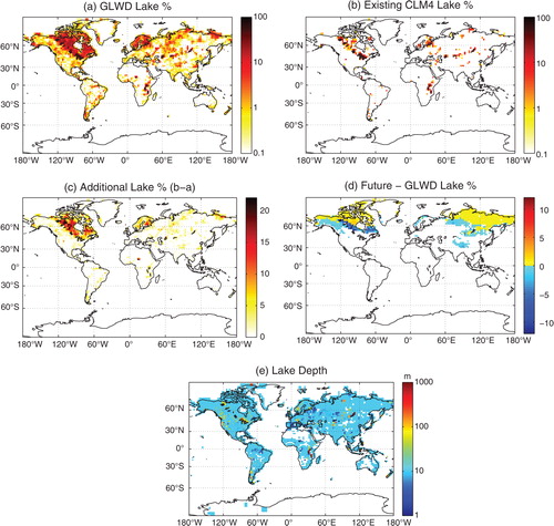
To characterise the effects of changing lake area in permafrost regions under climate change, we generated a potential future lake distribution dataset following the approach of Krinner and Boike (2010), who assumed that the area of inland water surfaces would decrease in disappearing permafrost by 40% but increase in areas of remaining permafrost by 10%. This assumption is qualitatively consistent with the modelling results of van Huissteden et al. (2011). However, whereas Krinner and Boike (2010) used climate model projections to predict these areas, we simply used the existing Brown et al. (2001) permafrost dataset and applied the 10% increase to areas currently classified as continuous permafrost and the 40% decrease to areas currently classified as containing discontinuous, sporadic and isolated permafrost. A key difference between our experiment and that of Krinner and Boike (2010) is that we considered only changes in lake area, whereas they combined changes in lake area with changes in wetland area in the same locations. The resulting 2.16 million km² of lake area (Fig. 1d) includes very small increases in northern Canada and northeast Asia and small decreases to the south, as compared to current conditions.

We used an interpolated version of a global gridded lake depth dataset (Kourzeneva, 2009 2010) (http://www.flake.igb-berlin.de/ep-data.shtml). This dataset includes real data for over 13 000 lakes, assigns a default depth of 10 m when a lake is present but depth data is not available and assigns a depth of 3 m for rivers. We interpolated this dataset to 1.9°×2.5° resolution using the mean depth from each 1 km grid cell, including those containing the default 10 m depth (Fig. 1e). As discussed in Subin et al. (2012), this interpolation is crude, as many grid cells are dominated by missing data, where the default depths are assigned. We consider this approach as an intermediate step between assuming a constant 50 m depth globally, as in the existing CLM4, and simulating several lakes of different size categories in each grid cell, as has been done for a regional climate model (Samuelsson et al., 2010).

2.3. Experimental design

We performed three primary CCSM4 experiments with two additional simulations for sensitivity to model version and forcing climate, and two idealised aqua-planet experiments described below. The primary experiments were intended to understand the sensitivity of present climate to lake distribution and the sensitivity of future climate to changes in lake distribution in permafrost regions, and they included a total of 10 CCSM4 simulations. These simulations were conducted using five combinations of climate and lake area (Table 1), with each combination using two model configurations (CLM4 offline and slab ocean modes) to separate the direct changes to surface fluxes caused by lakes from the atmospheric responses to these surface flux changes. The first experiment compared simulations using present climate with the GLWD lake area to simulations with the default CLM4 lake area (‘Hi’–‘Lo’), to see what biases may be introduced to the CCSM4 climate by using an unrealistically small lake area. The second experiment compared simulations using present climate with the GLWD lake area to simulations with no lake area at all (‘Hi’–‘No’), to compare with previous studies that have similarly investigated the seasonal effects of lakes on surface fluxes and regional climate (Bonan, 1995; Krinner, 2003; Dutra et al., 2010; Samuelsson et al., 2010). Finally, the third experiment compared simulations using future climate with the potential future lake distribution (Section 2.2) to simulations using future climate with the GLWD lake area (‘Fu_2CO₂’–‘Hi_2CO₂’).

Table 1. Community Climate System Model 4 (CCSM4) experimental design

	Lake area
Climate	Zero	CLM4	GLWD	Future
1850–2000^a		CCSM4-Historical^a
Eq. 2000	No	Lo; CCSM4-2000	Hi
Eq. 2×CO2			Hi_2CO 2	Fu_2CO 2

Notes: Each bold entry represents two simulations, one with CLM4 offline for 25 yr and one in slab ocean mode with equilibrium (Eq.) climate using fixed aerosol, greenhouse gas and ozone concentrations. The three primary experimental comparisons were Hi–Lo, Hi–No and Fu_2CO₂–Hi_2CO₂. Note that the offline CLM4 simulations with ‘2×CO₂’ actually used 2090–2099 atmospheric forcing from a previous RCP 4.5 simulation, as equilibrium doubled-CO₂ atmospheric forcing was not available. In addition, non-bold entries indicate simulations with the standard CCSM4, lacking CLM4-LISSS and the high-latitude biogeophysical changes.

^aThe CCSM4-Historical simulation was transient and included the full ocean model and CN.

For the simulations using present climate (No, Lo, and Hi), we spun up the land model for 100 yr using four cycles of 1980–2004 historical atmospheric forcing to equilibrate the lake temperatures, soil temperatures and soil moisture. The resulting land initial conditions were used for 25-yr simulations for the offline simulations and 200-yr simulations for the coupled simulations that used the standard year 2000 initial condition files for the atmosphere, slab ocean and sea ice. We discarded the first 20 yr of the coupled simulations to allow all the model components to equilibrate with the altered terrestrial surface and with fixed year 2000 atmospheric concentrations (i.e. ozone, aerosols, CO₂ and other greenhouse gases). Note that the short thermal relaxation time of the slab ocean means that we effectively simulated an equilibrium climate with year 2000 greenhouse gas concentrations, which will be warmer than observed conditions under transient greenhouse gas concentration increases, where net heat flux to the deep ocean cools the ocean surface and the atmosphere.

For the simulations using future climate (Hi_2CO₂ and Fu_2CO₂), we spun up the land model using 2090–2099 atmospheric forcing from a previous fully coupled CCSM4 RCP 4.5 simulation while retaining the standard year 2000 initial condition files for the other components. The offline simulations continued for another 25 yr using repeated 2090–2099 data. The fully coupled simulations using future climate were performed with all species kept at year 2000 concentrations except for CO₂, which was doubled over pre-industrial levels to 569.4 ppm. We ran these simulations for a total of 220 yr and discarded the first 40 yr to allow the land, sea ice and slab ocean additional time to equilibrate with the resulting climate.

To isolate the effects of model version and forcing climate on model predictions, we also performed two additional simulations (Table 1) with the standard version of CCSM4, which does not include CLM4-LISSS or the high-latitude biogeophysical changes. One simulation (‘CCSM4-2000’) was configured identically to the coupled simulations with slab ocean under present climate described above, except with only 100 yr of simulation, whereas the second (‘CCSM4-Historical’) consisted of a transient fully coupled CCSM4 simulation with POP2 from 1850 to 2000 with historical conditions for atmospheric constituents, land use, nitrogen deposition and aerosol deposition.

Finally, to better understand changes in large-scale atmospheric circulation and remote changes caused by the addition of mid- to high-latitude lake area, we also performed two idealised aqua-planet experiments mimicking the terrestrial surface forcing by perturbing prescribed SSTs from 40° to 70°N relative to a control simulation: (1) ‘SST-2’, a 2 °C cooling to resemble the effect of lakes in the summer; and (2) ‘SST + 2’, a 2 °C warming to resemble the effect of lakes in the fall. In the context of the hierarchy of models proposed by Held (2005), the use of aqua-planet allows the mechanisms of large-scale change to be more easily understood. The effects of terrestrial surface properties, topography, zonal asymmetry and seasonal cycles are removed, leaving a system that comes to equilibrium within 2 months and varies only on a synoptic time-scale.

2.4. Analysis

For the simulations using CLM4 offline, we calculated monthly anomalies for each of the three experiments for each of five surface fluxes: latent heat, sensible heat, net longwave emission, absorbed shortwave and subsurface energy flux (the rate of increase in snow, lake and soil enthalpy from both thermal diffusion at the surface and absorption of shortwave radiation). We examined these anomalies averaged over Canada (land north of 48°N and between 175° and 325°E). As the atmospheric forcing was fixed, there was no interaction of the lakes with internal variability, so no statistical analysis was needed.

For the coupled simulations, we calculated seasonal anomalies for each of the three experiments for: daily mean (T₂), maximum (T_max) and minimum (T_min) 2 m air temperature; diurnal 2 m air temperature range (DTR); convective, large-scale, and total precipitation; downwelling and absorbed shortwave radiation at the surface; low, medium, high and total cloud fraction; sea-level pressure (SLP); zonal and meridional wind; atmospheric temperature; geopotential height; and MSF. We highlighted statistically significant anomalies by doing a simple independent t-test for each grid cell or latitude (for zonally averaged fields) with a 5% significance threshold, with each 3-month season as one observation. However, we were cautious in interpreting significant changes remote from the locations of large lake area change. We compared DTR and precipitation for the simulations under present climate to the Climate Research Unit (CRU) 2.1 (Mitchell and Jones, 2005) climatology for the period 1980–2002. We also compared cloud fraction to the International Satellite Cloud Climatology Project D2 (ISCCP D2) (Rossow and Duenas, 2004) for the period 1984–2008.

We investigated whether either the mean states or variances of the NAO, NAM or ENSO were altered in the coupled experiments. For each season (for NAO, which is strongest during the winter and can vary on short timescales) or year (NAM and ENSO, which vary on multiyear timescales), we calculated the differences in SLP between the Azores and Iceland for NAO (Rogers, 1981), between 35°N and 65°N for NAM (Li and Wang, 2003) and between Tahiti and Darwin for ENSO (Trenberth, 1984), using grid cells within 2° of each point or latitude. We calculated the p-values of the independent t-statistic to detect differences in the means and the Bartlett statistic (Bartlett, 1937; Snedecor and Cochran, 1989) to detect differences in the variances. Because we performed 10 total tests, we adjusted the p-value required to detect significant changes down from 5% to 0.5% (1−0.95^1/10) to minimise the chance of a spurious significant result. We were also cautious in interpreting results, as some dynamic modes (i.e. ENSO) depend heavily on ocean dynamics that are not fully represented in slab ocean simulations. As a control, we also performed the same tests for differences between the Hi and Hi_2CO₂ simulations, where we may expect changes (Timmermann, 1999).

The three aqua-planet simulations were integrated for 3 yr, and we used the mean results for the last year in our analysis, calculating zonal mean anomalies with respect to the control simulation for total surface precipitation, 850 mb zonal windspeed and 500 mb geopotential height.

3. Results

3.1. Local effects of lake distribution

3.1.1. High (GLWD) versus low (CLM4 default) lake area under year 2000 climate (Hi–Lo).

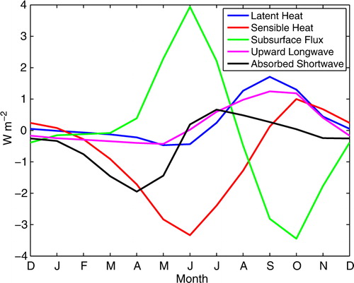
With fixed atmospheric forcing, the addition of 0.66 million km² of lake area in Canada caused up to 4.0 W m⁻² changes in monthly surface fluxes averaged over the region (Fig. 2). Subsurface energy absorption increased by an average of 2.2 W m⁻² from April through July; this energy was released back to the atmosphere at an average rate of 2.7 W m⁻² from September through November. There was an annual average shift of about 0.7 W m⁻² from sensible heat flux to latent heat flux and longwave emission. Lakes increased albedo during the spring melt more than they decreased albedo during the summer, causing a net annual decrease in absorbed shortwave radiation of 0.4 W m⁻².

Fig. 2.  Hi (GLWD lake area)–Lo (default CLM4 lake area) offline monthly average surface flux anomalies for Canada (land north of 48°N and between 175° and 325°E) under present climate: latent heat flux, sensible heat flux, rate of increase in subsurface enthalpy, upwelling longwave radiation and absorbed shortwave radiation. GLWD, Global Lake and Wetland Database.

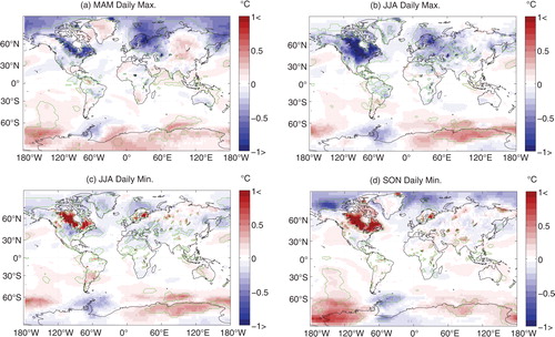
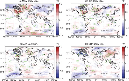
In coupled simulations, the increased subsurface thermal inertia and shift from sensible heat fluxes to latent heat and longwave fluxes caused widespread significant seasonal changes in T_min and T_max in Canada and Northern Europe (Fig. 3), with a maximum grid cell change of 2.3 °C (fall increase in T_min). In the spring and summer, warming and evaporating lakes caused a day-time cooling (Fig. 3a, b). During the summer and fall night time, lakes released heat back to the atmosphere and caused local warming (Fig. 3c, d). Near-surface relative humidity increased significantly by up to 6% in Central Canada in the summer.

Fig. 3.  Hi (GLWD lake area)–Lo (default CLM4 lake area) coupled seasonal average 2 m temperature anomalies under year 2000 conditions: (a) MAM daily maximum; (b) JJA daily maximum; (c) JJA daily minimum; and (d) SON daily minimum. Green contours encircle grid cells experiencing statistically significant changes. GLWD, Global Lake and Wetland Database.

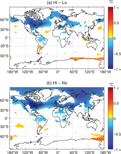
Significant T₂ changes in areas adjacent to added lakes were negative in the summer and positive in the fall, indicating a net uptake of energy by lakes during the summer and release to their surroundings in the fall. Moreover, the lower atmosphere is more tightly coupled to the terrestrial surface during the day than night and to sensible heat rather than longwave fluxes. Consequently, 850 hPa summer temperatures decreased by up to 1.2 °C over North America and the western North Atlantic (Fig. 4a). The mean summer planetary boundary layer (PBL) height decreased significantly by up to 70 m near the location of maximum decrease in 850 hPa temperature. This decrease is consistent with observations and modelling studies that show a lower PBL depth over wet locations (Banta and White, 2003; Patton et al., 2005) and with decreased sensible heat flux (Shin and Ha, 2007).

Fig. 4.  Significant JJA average atmospheric temperature anomalies at 850 hPa in coupled simulations under year 2000 conditions for (a) Hi (GLWD lake area)–Lo (default CLM4 lake area); and (b) Hi (GLWD lake area)–No (no lake area). GLWD, Global Lake and Wetland Database.

3.1.2. High (GLWD) versus no lake area under year 2000 climate (Hi–No)

With fixed atmospheric forcing, the replacement of vegetation and soil by lakes caused seasonal flux changes that depended on location. High-latitude lakes caused flux changes similar in sign to those resulting in the Hi–Lo experiment. Temperate lakes such as the Great Lakes, which were absent in the No simulation (but not the Lo simulation), stayed unfrozen into part of the winter season, increasing both sensible and latent heat fluxes. Tropical lakes were much smaller in extent but locally caused slight decreases in albedo, large decreases in sensible heat flux and large increases in latent heat flux for all seasons.

In coupled simulations, changes were similar in character to those for Hi–Lo, except larger in magnitude and broader in seasonal extent, especially in the vicinity of the Great Lakes. Downwelling shortwave radiation significantly decreased in the eastern US and Canada during all seasons due to increased cloudiness. The decrease in summer T_max over Great Lakes area grid cells was as large as 4.6 °C. Significant decreases in 850 hPa temperatures were widespread throughout North America, Russia, the Arctic and Europe and reached a magnitude of 2 °C above the Great Lakes (Fig. 4b). Winter T_min increased over the Great Lakes and to the east by ~1 °C.

3.1.3. Impacts of lake area changes from permafrost thaw under doubled CO₂ climate (Fu_2CO₂–Hi_2CO₂)

The assumed potential changes to future lake distribution resulting from permafrost thaw were small (Fig. 1d), with very small increases in northern Canada and Siberia contrasting with small decreases to the south. Consequently, resulting impacts on climate were small compared with the Hi–Lo experiment: the only region showing notable changes was the Canadian Shield that lost about 0.11 million km² of lake area. Changes in surface fluxes with fixed future atmospheric forcing were consistent in seasonality with Hi–Lo, except opposite in sign (because lakes were disappearing rather than being added) and smaller in magnitude. In coupled simulations, significant seasonal changes in T_min and T_max primarily occurred in the Canadian Shield (Fig. 5), with a maximum grid cell change of 1.3 °C (fall decrease in T_min). Northern Canada and Great Lakes spring and summer T_max increased (Fig. 5a, b), whereas summer and fall T_min decreased (Fig. 5c, d), opposite in sign to, and smaller in magnitude than the changes that occurred in Hi–Lo (Fig. 3).

Fig. 5.  Fu (potential future lake area)–Hi (GLWD lake area) coupled seasonal average 2 m temperature anomalies under doubled CO₂ conditions: (a) MAM daily maximum; (b) JJA daily maximum; (c) JJA daily minimum; and (d) SON daily minimum. Green contours encircle grid cells experiencing statistically significant changes. GLWD, Global Lake and Wetland Database.

3.2. Comparing predicted and observed DTR, precipitation and cloud cover (Hi–Lo)

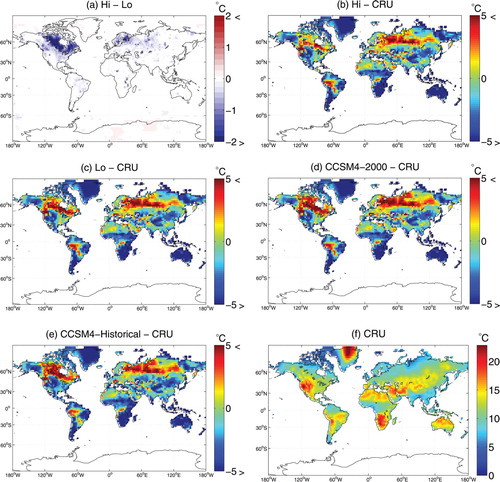
Increasing lake area to more realistic values caused significant decreases in predicted DTR throughout the spring, summer and fall in Canada and Scandinavia. Decreases were largest in the summer (Fig. 6a), up to 3.6 °C for individual grid cells. These decreases substantially reduced CCSM4 DTR biases compared to CRU in these affected areas (Fig. 6b, c), although large biases remained.

Fig. 6.  JJA diurnal 2 m temperature range: coupled anomalies for (a) Hi–Lo (significant only); (b) Hi–CRU; (c) Lo–CRU; (d) CCSM4-2000–CRU; and (e) CCSM4-Historical (1980–1999 mean)–CRU; and absolute JJA 2 m diurnal temperature range for (f) CRU (1980–2002). CCSM4, Community Climate System Model 4.

CCSM4 biases in precipitation and low clouds were slightly affected by the increase in lake area. Compared to ISCCP-D2, the Lo simulation underpredicted summer low cloud fraction in Canada and the Baltic by as much as 40%. We note that the summer low cloud bias in our simulations contrasted with the positive annual mean low cloud bias observed in the 1° CCSM4 (Gent et al., 2011). Low cloud fraction increased in the Hi simulation by up to 4%, significantly decreasing downward shortwave at the surface by ~3–9 W m⁻² and causing a slight improvement in the low cloud bias. Compared to CRU, the Lo simulation had a positive bias in total summer precipitation in the Central US of up to 4 mm d⁻¹. Convective precipitation significantly increased in the Hi simulation over the Central US by ~0.2 mm d⁻¹, whereas large-scale precipitation was unchanged, slightly worsening the total precipitation bias.

3.3. Aqua-planet simulations

As the mid- and high-latitude lake area increases decreased energy fluxes to the atmosphere in the summer and increased them in the fall (Fig. 2), we analysed the resulting remote effects via two idealised aqua-planet experiments with ±2 °C perturbed SSTs for 40–70°N (Fig. 7a). These perturbations caused changes in the tropics and the high-latitude SH. Generally, SST–2 and SST + 2 had opposite impacts. In the following analysis, we discuss changes in SST–2. The opposite analysis can be applied to changes in SST + 2 unless otherwise noted. The SST–2 induced a 2° northward shift of the ITCZ and a ~10% increase in its strength (Fig. 7b).

Fig. 7.  Zonally averaged fields for the three aqua-planet simulations: (a) prescribed SST for control, SST + 2 and SST–2; (b) precipitation anomalies with respect to control; (c) 850 mb zonal wind speed anomalies with respect to control; and (d) 500 mb geopotential height anomalies with respect to control.

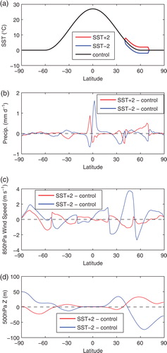
With NH extra-tropical surface cooling, the magnitude of the temperature gradient across the mid-latitudes increased. The NH Ferrell cell strengthened, associated with strengthening of the mid-latitude surface westerlies (Fig. 7c), increased subsidence at 30°N and increased ascent at 60°N (Fig. 7d). The NH Hadley Cell strengthened, associated with increased moisture transport from the subtropics to the tropics in the low level branch (not shown). Precipitation (Fig. 7b) increased just north of the equator. The mechanism linking the mid-latitude circulation changes to the tropical response will be detailed in a future study.

The ITCZ shift was associated with significant SH responses. The SST–2 northward shift in the ITCZ strengthened the subtropical jet and weakened the subsiding branch of the Hadley cell at 30°S (Fig. 7d). The mid-latitude surface westerlies were weakened (Fig. 7c). Southern Ocean surface winds were not changed in SST–2. In SST + 2, where the SH Hadley and Ferrell cells were strengthened, the westerlies strengthened in mid-latitudes and weakened at 60°S. Further work is required to understand why the SH zonal wind responses were not opposite in the SST–2 and SST + 2 scenarios.

3.4. Hi–Lo: large-scale and remote changes

3.4.1. Atmospheric circulation

Although the surface energy forcing caused by increased lake area in the Hi–Lo experiment was smaller in magnitude than the aqua-planet SST perturbations, due to both seasonal and zonal asymmetry, significant changes in atmospheric circulation and remote temperatures still occurred. Our analysis below focuses on changes in the summer and fall.

An increased summer NH meridional temperature gradient strengthened the upper tropospheric mid-latitude jet by ~0.50 m s⁻¹ between 40 and 50°N (Fig. 8a). While much smaller in magnitude, this change was consistent with changes found in the SST–2 experiment (Fig. 7c). Simulated meridional wind anomalies (not shown) may have indicated a NH wave train in response to changes in the jet (Liu and Alexander, 2007).

Fig. 8.  Significant seasonal average atmospheric zonal mean wind anomalies (+ to the east) in coupled simulations under year 2000 conditions for Hi (GLWD lake area)–Lo (default CLM4 lake area): (a) JJA, zonal mean; (b) SON, zonal mean; (c) SON, 850 hPa; and (d) SON, 200 hPa. GLWD, Global Lake and Wetland Database.

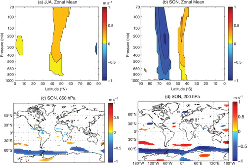
Small SH temperature changes occurred during the boreal summer (Fig. 4a). Significant differences in SH circulation also occurred in this season: increases of up to 1% in the SH tropical MSF indicated a weakened Hadley circulation, whereas decreases of up to 5% in the polar MSF indicated a strengthened polar cell. These changes in the MSF were consistent with the decreased subtropical and increased polar subsidence occurring in the SST–2 aqua-planet experiment (Fig. 7d). Hi–Lo changes in the summer MSF were not significant for the NH.

Significant changes in SH zonal winds occurred during the boreal fall (Fig. 8b, d). A decrease at the poleward edge and increase at the equatorward edge of mid-latitude westerlies resulted from an equatorward shift in the SH mid-latitude jet from 50°S to 45°S; at 60°S westerlies decreased by as much as 1 m s⁻¹. The geography of the westerly decreases followed the contours of the Southern Ocean, with 850 hPa winds decreasing by up to 0.7 m s⁻¹ (Fig. 8c). Significant changes of about 5% in the MSF (positive at 40°S and negative at 60°S) suggested both a strengthening Ferrell cell and a strengthening polar cell, with the boundary between the two shifting north. Increases in zonal mean SLP of up to 0.5 hPa south of 70°S also indicated a strengthened polar cell and were associated with regional temperature changes of up to 0.8°C (not shown). The zonal mean SH changes were consistent with the pattern in SST + 2 (Fig. 7c, d). Significant increases in the MSF of up to 3% between 5°N and 10°N may have indicated a slight southward shift in the ITCZ, consistent with the SST + 2 experiment. However, only slight zonal mean precipitation changes occurred of less than 0.1 mm d⁻¹.

3.4.2. Modes of variability

Changes in the mean and variance of the NAO, NAM or ENSO for Hi–Lo and Hi–No experiments were not significant at the 0.5% level. In contrast, we found highly significant (p<10⁻⁵) shifts in the annual mean phase of the NAO, NAM and ENSO in Hi_2CO₂ as compared to Hi, with a significant increase in winter NAO variance.

4. Discussion

4.1. Effects of lakes on seasonal surface fluxes and local air temperature

As discussed in Subin et al. (2012), previous studies (Bonan, 1995; Lofgren, 1997; Krinner, 2003; Rouse et al., 2005; Long et al., 2007; Dutra et al., 2010; Samuelsson et al., 2010) have largely agreed on the seasonal effects of lakes on local surface energy fluxes and surface air temperature, with some disagreement as to the net effect on latent heat flux and air temperature at high latitudes in the summer, and whether atmospheric warming persists into the winter after lakes have frozen. The summer disagreements may be related to how dry the neighbouring soil is simulated to be (Krinner and Boike, 2010) and how the vegetation is represented there. The winter disagreements may depend on the presence and extent of snow insulation in the model (Dutra et al., 2010).

Local changes in seasonal T₂ in the Hi–Lo, Hi–No and Fu_2CO₂–Hi_2CO₂ experiments were within the range of those reported in previous studies. We found that high-latitude lakes caused net local cooling in the spring and summer, and net warming in the fall. Slight net cooling during the summer resulted from the balance of day-time cooling and night-time warming, with slight increases in latent heat flux and longwave emission, and large decreases in sensible heat flux. Some studies (Krinner, 2003; Dutra et al., 2010) have found decreases in summer latent heat flux due to lower surface temperatures and decreased roughness lengths. We also found slight decreases in latent heat flux in the early summer; the largest contribution to summer decreased sensible heat flux at high latitudes was increased energy uptake by lakes, not increased latent heat flux.

In the winter, we found that high-latitude lakes did not cause significant warming; this was likely due to the inclusion of snow insulation in CLM4-LISSS (Dutra et al., 2010; Subin et al., 2012). Although CCSM4 moderately overpredicts snow depth at high latitudes due to excessive winter precipitation (Lawrence et al., 2011b), offline CLM4 slightly underpredicts high-latitude snow cover fraction (Lawrence et al., 2011a) and lakes caused little change in winter surface fluxes in the offline Hi–Lo experiment. At lower latitudes, the Great Lakes remained unfrozen for part of the winter in the coupled Hi simulation, causing significant winter warming in this region compared to the coupled No simulation.

4.2. Implications for CCSM4 Evaluation

While most CMIP3 climate models underestimated DTR throughout land areas (Randall et al., 2007), we found that CCSM4 overestimated summer DTR in boreal regions (Fig. 6c), including regions where lake area is underestimated (Fig. 1b, c). This overestimation was due to both excessively high T_max and low T_min (not shown). This bias was reduced in those regions when more realistic lake area was used (Fig. 6a, b), although it was not eliminated. As the T₂ changes in our experiments and those of Krinner and Boike (2010) were linear with lake area change and independent of baseline climate, we hypothesise that increasing lake area to the values suggested to be realistic by Downing et al. (2006) would further reduce the DTR bias. However, the concurrent underestimation in simulated low cloud fraction may also have contributed to the high DTR bias (Dai et al., 1999). Indeed, some of the decrease in DTR with more realistic lake area may have resulted indirectly from the increase in low cloud fraction rather than the direct effect of lakes on surface energy fluxes.

Using the CCSM4-2000 and CCSM4-Historical simulations, we investigated the sensitivity of DTR biases to the model version and the climate forcing. The CCSM4-2000 simulation differed from the coupled Lo simulation only in duration and in lacking CLM4-LISSS and the high-latitude biogeophysical changes under development by S. C. Swenson and D. M. Lawrence. The positive summer DTR bias was larger in boreal regions in CCSM4-2000 than in the Lo simulation (Fig. 6d), notably in the Great Lakes region. This finding is consistent with the existing CLM4 lake model deficiencies, including excessive surface diurnal temperature range (Subin et al., 2012). However, much of the improvement in permafrost regions in the Lo simulation may have resulted from the biogeophysical changes.

The simulations using equilibrium 2000 conditions with slab ocean should have had a slightly warmer atmosphere than the 1980–2002 period, both due to changes between 1980 and 2000 and the lack of transient heat flux to the deep ocean. Consequently, interactions between DTR and atmospheric warming could have caused the simulated DTR to differ from the CRU observations. To test the importance of this caveat, we evaluated the summer DTR predicted in the CCSM4-Historical simulation during 1980–1999 (Fig. 6e). We found that the positive DTR bias, although slightly lower in some regions than in the CCSM4-2000 simulation, remained large in almost all regions with unrealistic lake area.

While increasing lake area in the Hi–Lo experiment slightly improved the large negative bias in summer low cloud fraction in Canada, even larger improvements occurred over Arctic land when we compared the Lo simulation to the CCSM4-2000 simulation, likely related to the high-latitude biogeophysical changes. The negative summer low cloud fraction bias was improved over the Great Lakes in CCSM4-Historical relative to CCSM4-2000, but not elsewhere at high latitudes. The bias towards excessive summer precipitation in the Central US plains in the Lo simulation (which was slightly worsened in the Hi simulation) was unchanged in the CCSM4-2000 simulation but larger in the CCSM4-Historical simulation.

Assessing improvements to GCM simulations after changing one model component is difficult; compensating errors may cause a reduction in bias for the wrong reasons. We cannot be confident that the reduced DTR bias from adding lake area did not either come at the expense of other hydroclimate variables or compensate for other sources of bias; further work should investigate the DTR bias in CCSM4 and other CMIP5 climate models more systematically. As long as there are no interactions between lake area change and model biases, our predicted changes in climate variables with the addition of lake area will be relatively robust. Biases that would interact with lake area change include unrealistic soil moisture or stomatal limitation of ET in areas replaced by lakes, or an unrealistic land–atmosphere coupling strength. CCSM4 tends to have excessive summer soil moisture limitation in permafrost regions (Lawrence et al., 2011b), which would tend to increase the effects of adding lakes. However, CCSM4 tends to have excessive transpiration (Lawrence et al., 2011b) and a relatively weak land–atmosphere coupling strength (D. M. Lawrence, personal communication, 2011) in tropical and temperate regions, which would tend to reduce the effects of adding lakes.

4.3. Climate effects of changing lake area in permafrost regions

We found that decreasing lake area in regions currently characterised by discontinuous permafrost could cause mild seasonal changes in T₂, up to a 1.3 °C decrease in T_min. However, these changes were modest compared to the biases that may result in the simulation of current climate from using unrealistically small lake area. Krinner and Boike (2010) found significant changes consistent in seasonal sign but somewhat larger and more widespread. These slightly larger changes were likely because they considered the combined disappearance of lake and wetland area, whereas we considered only changes in lake area. Differences in present and future lake area distributions and lake model structure and parameterisation were not likely causes of the discrepancy, except during the winter season, when Krinner and Boike (2010) found significant winter cooling from decreased inland water surface area. We did not find significant winter impacts of lakes at high latitudes, as discussed in Section 4.1.

Our simulations could underestimate the climate impacts of changing lakes in permafrost regions. While we followed the assumption of Krinner and Boike (2010) [based loosely on the analysis by Smith et al. (2007) and consistent with the observations in Plug et al. (2008) and simulations by van Huissteden et al. (2011)] that lake area in remaining or currently continuous permafrost would only increase by 10%, it is possible that thermokarst activity could increase lake area by larger percentages in some regions. Our estimates are also sensitive to our assumed existing high-latitude lake area, which is likely an underestimate (Downing et al., 2006). Moreover, we have only considered the physical impacts of changing lake area. The biogeochemical impact of expanding thermokarst lakes and increasing emissions of CO₂ and CH₄ from these lakes is more difficult to quantify (Wania et al., 2010; Riley et al., 2011) and may be large (Walter et al., 2007; Schuur et al., 2008).

4.4. Large-scale changes resulting from mid- and high-latitude NH surface forcing

Shifts in the ITCZ in response to decreases in NH extra-tropical surface temperatures in our aqua-planet experiments were in the opposite direction of those predicted by previous studies (Kang et al., 2008 2009), likely due to our use of prescribed SSTs rather than a slab ocean model. We hypothesise that this difference is representative of some differences in the atmospheric responses to terrestrial rather than ocean cooling. We highlight two of these differences: (1) a cooling due to a change in ocean circulation would imply a compensating remote warming [e.g. Kang et al. (2008 2009) imposed an implied cross-equatorial subsurface heat flux], whereas a cooling due to a change in terrestrial surface properties (e.g. albedo) may decrease the top-of-atmosphere energy balance without a direct compensation elsewhere; (2) an ocean cooling would generally persist for a long enough time for remote ocean temperatures to respond, whereas a terrestrial cooling, such as that resulting from increased subsurface energy storage due to increased lake area, may be seasonal or otherwise transient. We may tentatively reject (1) as an explanation: while the cross-equatorial heat flux imposed in Kang et al. (2008 2009) may have reinforced the southward ITCZ shift, several other studies (Chiang and Bitz, 2005; Lee et al., 2011) found a southward ITCZ shift from extra-tropical NH cooling without imposing any compensating cross-equatorial heat flux. In particular, the Chiang and Bitz (2005) experiment simulated the responses to an increase in Arctic sea ice, which may act similarly to an increase in terrestrial albedo. However, regarding (2), we are not aware of previous studies investigating the transient response to extra-tropical cooling, so it is possible that the initial atmospheric response would be different in character than the equilibrium response once tropical SSTs have adjusted to the forcing. Further research should investigate these potentially contrasting responses.

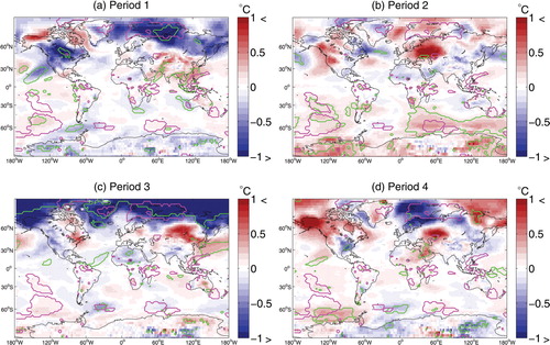
Interpreting significant changes in geographic fields at the grid cell level requires caution due to spatial and temporal autocorrelation. To illustrate the limitations of using relatively short simulations to detect signals smaller than typical inter-annual variability, we divided the 180 yr analysed for the Hi–Lo experiment into four 45-yr periods, and we compared statistical significance evaluated for each individual period with that evaluated for the entire period. Even in the winter, when the surface forcing caused by the addition of lakes was small (Fig. 2), some regions with statistically significant changes occurred when evaluated over the entire 180-yr period (Fig. 9). However, the changes in individual periods within these regions were not always consistent in sign or significant: the Barents Sea cooled in three of the periods but warmed in the fourth. Moreover, the regions appearing to be significant in each period were not always contained within the regions found to be significant for the entire 180-yr period. In particular, most of the Arctic experienced an apparently statistically significant cooling of 1 °C or more during one of the periods (‘Period 3’, Fig. 9c), but this cooling did not occur during the other three periods. We note that the previously discussed significant changes occurring in the summer and fall showed much more consistency among the four periods than the winter changes in Fig. 9.

Fig. 9.  Hi (GLWD lake area)–Lo (default CLM4 lake area) coupled DJF 2 m temperature anomalies under year 2000 conditions for the four 45-yr periods composing the full 180 analysed years of simulation: (a) Period 1; (b) Period 2; (c) Period 3; and (d) Period 4. Green contours encircle significant changes evaluated for each 45-yr period, whereas magenta contours encircle regions where significant changes were found for the full 180 yr. GLWD, Global Lake and Wetland Database.

Because of these challenges in interpreting statistically significant changes, we have attempted to be cautious in interpreting remote changes such as the Hi–Lo SH changes in boreal summer temperature and boreal fall zonal winds by examining whether changes were mechanistically consistent among several variables (e.g. temperature, pressure, wind and MSF), linked to changes in the NH tropics, and similar to analogous changes in the idealised aqua-planet simulations. Many of the remote changes occurring in Hi–Lo failed to satisfy all these criteria, including some localised changes in temperature, precipitation and surface pressure that we did not analyse in Section 3.4.1. The changes in zonal winds in the boreal summer and fall may be the most compelling. Both the summer increases in NH mid-latitude westerlies and the boreal fall decreases in Southern Ocean westerlies were consistent among several variables and with the analogous aqua-planet experiments, although changes in the NH tropics were very small compared to changes in the aqua-planet experiments. We note that many terrestrial surface changes associated with climate change (e.g. vegetation distribution changes, loss of land ice or snow cover or changes in wetland area) may be of much larger magnitude than the lake area changes simulated here. Although previous studies may have used simulations of insufficient duration to detect remote changes, our results suggest that these changes may be significant.

5. Conclusions

The presence of large lake area in boreal regions, particularly the Canadian Shield, causes widespread changes in North American surface air temperatures of 1–2 °C during the spring, summer and fall, as compared to a comparable system with much less lake area. Increased subsurface thermal inertia reduces diurnal temperature variation, causes increases in low cloud fraction and causes net spring and summer cooling and fall warming. Increasing the realism of modelled lake area and properties in climate models may improve simulated biases in diurnal temperature range in some regions, although this evaluation is complicated by the large number of processes affecting diurnal temperature range.

Relatively small changes of 2 °C in extra-tropical surface temperatures can cause changes in atmospheric circulation and remote precipitation and winds, although realistic zonally and seasonally asymmetric forcings have less coherent impacts than idealised forcings of similar maximum magnitude. A consistent response to increases in extra-tropical Northern Hemisphere surface energy fluxes in our experiments was decreases in westerly flow over the Southern Ocean; according to previous analyses, these changes could alter ocean upwelling and affect the global carbon cycle. A more detailed investigation of this mechanism is warranted. Further research is also needed to understand potentially contrasting atmospheric responses to extra-tropical surface temperature changes depending on the character of the imposed forcing and remote ocean responses.

The disappearance of lakes from present regions of discontinuous permafrost could cause small (0.5–1 °C) changes in surface air temperature in certain regions, such as central northern Canada, increasing diurnal temperature variation and amplifying summer warming. However, these changes may be relatively small compared to the effects of global climate change in the same regions or to errors in simulation caused by the underestimation of lake area in current datasets. To confirm this, research should focus on improving datasets of existing high-latitude lake area and improving understanding of the potential for increases in lake area due to thermokarst activity in remaining permafrost regions. Furthermore, the biogeochemical changes associated with melting permafrost are likely more uncertain than the direct physical responses to changes in lake area.

6. Acknowledgements

Michael Wehner (Lawrence Berkeley National Lab), John Chiang (University of California, Berkeley), Benjamin Santer (Lawrence Livermore National Lab), William Collins (Lawrence Berkeley National Lab) and Sarah Kang (Columbia University) provided helpful comments on interpreting large-scale atmospheric responses to regional changes in terrestrial surface forcing. David Lawrence (National Center for Atmospheric Research) facilitated interaction with the CESM Land Model Working Group and support in running and interpreting the model. One anonymous reviewer and one named reviewer (Sumant Nigam) provided helpful comments in clarifying and improving the manuscript. This work was supported by the Director, Office of Science, Office of Biological and Environmental Research, Climate and Environmental Science Division, of the US Department of Energy under Contract No. DE-AC02-05CH11231 to Berkeley Lab.

References

- Anderson, R. F, Ali, S, Bradtmiller, L. I, Nielsen, S. H. H, Fleisher, M. Q and co-authors. 2009. Wind-driven upwelling in the southern ocean and the deglacial rise in atmospheric CO2. Science. 323, 1443–1448.
- Banta R. M. White A. B. Mixing-height differences between land use types: dependence on wind speed. J. Geophys. Res. 2003; 108: 4321.
- Bartlett M. S. Properties of sufficiency and statistical tests. Proc. R. Soc. Lond. Ser. A. 1937; 160: 268–282.
- Bates G. T. Giorgi F. Hostetler S. W. Towards the simulation of the effects of the great-lakes on regional climate. Mon. Weather Rev. 1993; 121: 1373–1387.
- Bonan G. B. Sensitivity of a GCM simulation to inclusion of inland water surfaces. J. Clim. 1995; 8: 2691–2704.
- Bonfils, C, Angert, A, Henning, C. C, Biraud, S, Doney, S. C and co-authors. 2005. Extending the record of photosynthetic activity in the eastern United States into the presatellite period using surface diurnal temperature range. Geophy. Res. Lett. 32, L08405.
- Bonfils C. Santer B. Investigating the possibility of a human component in various pacific decadal oscillation indices. Clim. Dyn. 2010; 37: 1457–1468.
- Braganza, K, Karoly, D. J and Arblaster, J. M. 2004. Diurnal temperature range as an index of global climate change during the twentieth century. Geophys. Res. Lett. 31, L13217.
- Branstator G. Circumglobal teleconnections, the jet stream waveguide, and the North Atlantic oscillation. J. Clim. 2002; 15: 1893–1910.
- Brown L. C. Duguay C. R. The response and role of ice cover in lake-climate interactions. Prog. Phys. Geogr. 2010; 34: 671–704.
- Brown, J, Ferrians, O. J. J, Heginbottom, J. A and Melnikov, E. S. 2001. Circum-Arctic Map of Permafrost and Ground-Ice Conditions. National Snow and Ice Data Center/World Data Center for Glaciology. http://nsidc.org/data/ggd318.html.
- Chase T. N. Pielke R. A. Kittel T. G. F. Nemani R. R. Running S. W. Simulated impacts of historical land cover changes on global climate in northern winter. Clim. Dyn. 2000; 16: 93–105.
- Chiang J. C. H. Bitz C. M. Influence of high latitude ice cover on the marine Intertropical Convergence Zone. Clim. Dyn. 2005; 25: 477–496.
- Cogley, J. G. 1991. GGHYDRO – Global Hydrographic Data Release 2.0.. Department of Geography, Trent University, Peterborough, Ontario. Trent Climate Note 91-1.
- Collatz, G. J, Bounoua, L, Los, S. O, Randall, D. A, Fung, I. Y and co-authors. 2000. A mechanism for the influence of vegetation on the response of the diurnal temperature range to changing climate. Geophys. Res. Lett. 27, 3381–3384.
- Collins, W. D, Rasch, P. J, Boville, B. A, Hack, J. J, McCaa, J. R and co-authors. 2004. Description of the NCAR Community Atmosphere Model (CAM3). National Center for Atmospheric Research, NCAR/TN-485 + STR, Boulder, CO.
- Corti S. Molteni F. Palmer T. N. Signature of recent climate change in frequencies of natural atmospheric circulation regimes. Nature. 1999; 398: 799–802.
- Dai A. Trenberth K. E. Karl T. R. Effects of clouds, soil moisture, precipitation, and water vapor on diurnal temperature range. J. Clim. 1999; 12: 2451–2473.
- Delworth T. L. Mann M. E. Observed and simulated multidecadal variability in the Northern Hemisphere. Clim. Dyn. 2000; 16: 661–676.
- Downing, J. A, Prairie, Y. T, Cole, J. J, Duarte, C. M, Tranvik, L. J and co-authors. 2006. The global abundance and size distribution of lakes, ponds, and impoundments. Limnol. Oceanogr. 51, 2388–2397.
- Dutra, E, Stepanenko, V. M, Balsamo, G, Viterbo, P, Miranda, P. M. A and co-authors. 2010. An offline study of the impact of lakes on the performance of the ECMWF surface scheme. Boreal Env. Res. 15, 100–112.
- Fang X. Stefan H. G. Long-term lake water temperature and ice cover simulations/measurements. Cold Reg. Sci. Tech. 1996; 24: 289–304.
- Feddema, J. J, Oleson, K. W, Bonan, G. B, Mearns, L. O, Buja, L. E and co-authors. 2005a. The importance of land-cover change in simulating future climates. Science. 310, 1674–1678.
- Feddema, J, Oleson, K. W, Bonan, G. B, Mearns, L. O, Washington, W and co-authors. 2005b. A comparison of a GCM response to historical anthropogenic land cover change and model sensitivity to uncertainty in present-day land cover representations. Clim. Dyn. 25, 581–609.
- Frankcombe L. M. Dijkstra H. A. Internal modes of multidecadal variability in the Arctic ocean. J. Phys. Oceanogr. 2010; 40: 2496–2510.
- Geerts B. Empirical estimation of the monthly-mean daily temperature range. Theoret. Appl. Clim. 2003; 74: 145–165.
- Gent, P. R, Danabasoglu, G, Donner, L. J, Holland, M. M, Hunke, E. C and co-authors. 2011. The community climate system model version 4. J. Clim. 24, 4973–4991.
- Gent P. R. Yeager S. G. Neale R. B. Levis S. Bailey D. A. Improvements in a half degree atmosphere/land version of the CCSM. Clim. Dyn. 2010; 34: 819–833.
- Goyette S. McFarlane N. Flato G. Application of the Canadian Regional Climate Model to the Laurentian Great Lakes Region: implementation of a lake model. Atmosphere-Ocean. 2000; 38: 481–503.
- Graham N. E. White W. B. The El-Nino Cycle – a natural oscillator of the Pacific-Ocean atmosphere system. Science. 1988; 240: 1293–1302.
- Grosse, G, Romanovsky, V. E, Walter, K. M, Morgenstern, A, Lantuit, H and co-authors. 2008. Distribution of Thermokarst Lakes and Ponds at Three Yedoma Sites in Siberia. In: Proceedings of the 9th International Conference on Permafrost, Fairbanks, University of Alaska, June 29–July 3, 2008, 551–556.
- Guan B. Nigam S. Analysis of Atlantic SST variability factoring interbasin links and the secular trend: clarified structure of the atlantic multidecadal oscillation. J. Clim. 2009; 22: 4228–4240.
- Guo, Z, Dirmeyer, P. A, Koster, R. D, Bonan, G, Chan, E and co-authors. 2006. GLACE: the global land-atmosphere coupling experiment. Part II: analysis. J. Hydrometeor. 7, 611–625.
- Held I. M. The gap between simulation and understanding in climate modeling. Bullet. Amer. Meteorol. Soc. 2005; 86: 1609–1614.
- Held I. M. Ting M. F. Wang H. L. Northern winter stationary waves: theory and modeling. J. Clim. 2002; 15: 2125–2144.
- Holton J. R. An Introduction to Dynamic Meteorology. Elselvier Academic Press: San Diego CA, 2004
- Hoskins B. J. Karoly D. J. The steady linear response of a spherical atmosphere to thermal and orographic forcing. J. Atmos. Sci. 1981; 38: 1179–1196.
- Hostetler S. Bartlein P. Simulation of Lake Evaporation with application to modeling Lake level variations of Harney-Malheur Lake, Oregon. Water Resour. Res. 1990; 26: 2603–2612.
- Jorgenson M. T. Racine C. H. Walters J. C. Osterkamp T. E. Permafrost degradation and ecological changes associated with a warming climate in central Alaska. Clim. Change. 2001; 48: 551–579.
- Jorgenson M. T. Shur Y. L. Pullman E. R. Abrupt increase in permafrost degradation in Arctic Alaska. Geophys. Res. Lett. 2006; 33: L02503.
- Kaab A. Haeberli W. Evolution of a high-mountain thermokarst lake in the Swiss Alps. Arctic Antarctic and Alpine Res. 2001; 33: 385–390.
- Kalnay E. Cai M. Impact of urbanization and land-use change on climate. Nature. 2003; 423: 528–531.
- Kang S. M. Held I. M. Frierson D. M. W. Zhao M. The response of the ITCZ to extratropical thermal forcing: idealized slab-ocean experiments with a GCM. J. Clim. 2008; 21: 3521–3532.
- Kang S. M. Frierson D. M. W. Held I. M. The tropical response to extratropical thermal forcing in an idealized GCM: the importance of radiative feedbacks and convective parameterization. J. Atmos. Sci. 2009; 66: 2812–2827.
- Karl, T. R, Jones, P. D, Knight, R. W, Kukla, G, Plummer, N and co-authors. 1993. A new perspective on recent global warming- asymmetric trends of daily maximum and minimum temperature. Bullet. Amer. Meteorol. Soc. 74, 1007–1023.
- Kawamura R. A Rotated EOF analysis of global sea-surface temperature variability with interannual and interdecadal scales. J. Phys. l Oceanogr. 1994; 24: 707–715.
- Kourzeneva, E. 2009. Global dataset for the parameterization of lakes in numerical weather prediction and climate modeling. In: ALADIN Newsletter. F. Bouttier and C. Fischer. ToulouseFrance: Meteo-France. pp. 46–53.
- Kourzeneva E. External data for lake parameterization in Numerical Weather Prediction and climate modeling. Boreal Env. Res. 2010; 15: 165–177.
- Krinner G. Impact of lakes and wetlands on boreal climate. J. Geophys. Res. 2003; 108: 18.
- Krinner G. Boike J. A study of the large-scale climatic effects of a possible disappearance of high-latitude inland water surfaces during the 21st century. Boreal Env. Res. 2010; 15: 203–217.
- Kristovich D. A. R. Braham R. R. Mean profiles of moisture fluxes in snow-filled boundary layers. Boundary-Layer Meteorol. 1998; 87: 195–215.
- Kushnir Y. Wallace J. M. Low-frequency variability in the northern hemisphere winter – geographical-distribution, structure and time-scale dependence. J. Atmos. Sci. 1989; 46: 3122–3142.
- Kutzbach J. E. Large-scale features of monthly mean northern hemisphere anomaly maps of sea-level pressure. Month. Wea. Rev. 1970; 98: 708–716.
- Laird N. F. Desrochers J. Payer M. Climatology of lake-effect precipitation events over lake champlain. J. Appl. Meteorol. Climatol. 2009; 48: 232–250.
- Lawrence, D. M, Oleson, K. W, Flanner, M. G, Fletcher, C. G, Lawrence, P. J and co-authors. 2011b. The CCSM4 land simulation, 1850–2005: assessment of surface climate and new capabilities. J. Clim. CCSM4 Special Collection. doi: 10.1175/JCLI-D-11-00103.1 (online first).
- Lawrence, D, Oleson, K. W, Flanner, M. G, Thorton, P. E, Swenson, S. C and co-authors. 2011a. Parameterization improvements and functional and structural advances in version 4 of the community land model. J. Adv. Model. Earth Sys. 3, 27.
- Lee S.-Y. Chiang J. C. H. Matsumoto K. Tokos K. S. Southern Ocean wind response to North Atlantic cooling and the rise in atmospheric CO2: modeling perspective and paleoceanographic implications. Paleoceanography. 2011; 26: PA1214.
- Lehner B. Döll P. Development and validation of a global database of lakes, reservoirs and wetlands. J. Hydrol. 2004; 296: 1–22.
- Levitus S. Matishov G. Seidov D. Smolyar I. Barents sea multidecadal variability. Geophys. Res. Lett. 2009; 36: 5.
- Li, F, Collins, W. D, Wehner, M. F, Williamson, D. L, Olson, J. G and co-authors. 2011. Impact of horizontal resolution on simulation of precipitation extremes in an aqua-planet version of Community Atmospheric Model (CAM3). Tellus A, 63, 884–892.
- Li, J. P and Wang, J. 2003. A modified zonal index and its physical sense. Geophys. Res. Lett. 30, 1632.
- Linkin M. E. Nigam S. The north pacific oscillation-west Pacific teleconnection pattern: mature-phase structure and winter impacts. J. Clim. 2008; 21: 1979–1997.
- Liu, Z. Y and Alexander, M. 2007. Atmospheric bridge, oceanic tunnel, and global climatic teleconnections. Rev. Geophys. 45, RG2005.
- Livezey R. E. Chen W. Y. Statistical field significance and its determination by monte-carlo techniques. Month. Wea. Rev. 1983; 111: 46–59.
- Lofgren B. M. Simulated effects of idealized Laurentian Great Lakes on regional and large-scale climate. J. Clim. 1997; 10: 2847–2858.
- Lofgren, B. M. 2004. A model for simulation of the climate and hydrology of the Great Lakes basin. J. Geophys. Res. 109, D18108.
- Long Z. Perrie W. Gyakum J. Caya D. Laprise R. Northern lake impacts on local seasonal climate. J. Hydrometeorol. 2007; 8: 881–896.
- Minobe S. A 50-70 year climatic oscillation over the North Pacific and North America. Geophys. Res. Lett. 1997; 24: 683–686.
- Mitchell T. D. Jones P. D. An improved method of constructing a database of monthly climate observations and associated high-resolution grids. Int. J. Clim. 2005; 25: 693–712.
- Neale R. B. Hoskins B. J. A standard test for AGCMs including their physical parametrizations: I: the proposal. Atmos. Sci. Lett. 2000; 1: 101–107.
- Neale, R. B, Richter, J. H, Conley, A. J, Park, S, Lauritzen, P. H and co-authors. 2010. Description of the NCAR Community Atmosphere Model (CAM 4.0). National Center for Atmospheric Research, NCAR/TN-485 + STR, Boulder, CO.
- Neale R. B. Richter J. H. Jochum M. The impact of convection on ENSO: from a delayed oscillator to a series of events. J. Clim. 2008; 21: 5904–5924.
- Nigam, S. 2003. Teleconnections. In: Encyclopedia of Atmospheric Sciences. R. H. James. Oxford: Academic Press. pp. 2243–2269.
- Nigam, S and DeWeaver, E. 2003. Stationary waves (orographic and thermally forced). In: Encyclopedia of Atmospheric Sciences. R. H. James. Oxford: Academic Press. pp. 2121–2137.
- Nigam S. Lindzen R. S. The sensitivity of stationary waves to variations in the basic state zonal flow. J. Atmos. Sci. 1989; 46: 1746–1768.
- Nigam S. Ruiz-Barradas A. Seasonal hydroclimate variability over north America in global and regional reanalyses and AMIP simulations: varied representation. J. Clim. 2006; 19: 815–837.
- Ogi M. Yamazaki K. Trends in the summer northern annular mode and Arctic sea ice. Sola. 2010; 6: 41–44.
- Oleson, K, Lawrence, D. M, Bonan, G. B, Flanner, M. E. K, Lawrence, P and co-authors. 2010. Technical description of version 4.0 of the Community Land Model (CLM). National Center for Atmospheric Research, NCAR/TN-485 + STR, Boulder, CO.
- Oort A. H. Rasmusson E. M. On annual variation of monthly mean meridional circulation. Month. Wea. Rev. 1970; 98: 423–442.
- Patton E. G. Sullivan P. P. Moeng C. H. The influence of idealized heterogeneity on wet and dry planetary boundary layers coupled to the land surface. J. Atmos. Sci. 2005; 62: 2078–2097.
- Plug L. J. Walls C. Scott B. M. Tundra lake changes from 1978 to 2001 on the Tuktoyaktuk Peninsula, western Canadian Arctic. Geophys. Res. Lett. 2008; 35: 5.
- Polyakov, I. V, Bekryaev, R. V, Alekseev, G. V, Bhatt, U. S, Colony, R. L and co-authors. 2003. Variability and trends of air temperature and pressure in the maritime Arctic, 1875–2000. J. Clim. 16, 2067–2077.
- Polyakov I. V. Johnson M. A. Arctic decadal and interdecadal variability. Geophys. Res. Lett. 2000; 27: 4097–4100.
- Qian T. T. Dai A. G. Trenberth K. E. Oleson K. W. Simulation of global land surface conditions from 1948 to 2004. Part I: forcing data and evaluations. J. Hydrometeorol. 2006; 7: 953–975.
- Randall, D. A.,Wood, R. A.,Bony, S.,Colman, R.,Fichefet, T and co-authors. 2007. Climate models and their evaluation. In: Climate Change 2007: The Physical Science Basis. Contribution of Working Group I to the Fourth Assessment Report of the Intergovernmental Panel on Climate Change. S. Solomon, D. Qin, M. Manning, Z. Chen, M. Marquis, K. B. Averyt, M. Tignor and H. L. Miller. Cambridge University Press: Cambridge. pp. 589–662.
- Richter J. H. Rasch P. J. Effects of convective momentum transport on the atmospheric circulation in the community atmosphere model, version 3. J. Clim. 2008; 21: 1487–1499.
- Riley, W. J, Subin, Z. M, Lawrence, D. M, Swenson, S. C, Torn, M. S, Meng, L and co-authors. 2011. Barriers to predicting changes in global terrestrial methane fluxes: analyses using CLM4Me, a methane biogeochemistry model integrated in CESM. Biogeosciences. 8, 1925–1953.
- Riordan B. Verbyla D. McGuire A. D. Shrinking ponds in subarctic Alaska based on 1950–2002 remotely sensed images. J. Geophys. Res. 2006; 111: 11.
- Rogers J. C. Spatial variability of seasonal sea-level pressure and 500 mb height anomalies. Month. Wea. Rev. 1981; 109: 2093–2106.
- Rossow W. B. Duenas E. N. The International Satellite Cloud Climatology Project (ISCCP) web site – an online resource for research. Bullet. Amer. Meteorol. Soc. 2004; 85: 167–172.
- Rouse, W. R, Blanken, P. D, Bussieres, N, Oswald, C. J, Schertzer, C and co-authors. 2008. Investigation of the thermal and energy balance regimes of great slave and great bear lakes. J. Hydrometeorol. 9, 1318–1333.
- Rouse, W. R, Oswald, C. J, Binyamin, J, Spence, C. R, Schertzer, W. M and co-authors. 2005. The role of northern lakes in a regional energy balance. J. Hydrometeorol. 6, 291–305.
- Samuelsson P. Kourzeneva E. Mironov D. The impact of lakes on the European climate as simulated by a regional climate model. Boreal Env. Res. 2010; 15: 113–129.
- Samuelsson P. Tjernström M. Mesoscale flow modification induced by land-lake surface temperature and roughness differences. J. Geophys. Res. 2001; 106: 12419–12435.
- Schindler D. W. Lakes as sentinels and integrators for the effects of climate change on watersheds, airsheds, and landscapes. Limnol. Oceanogr. 2009; 54: 2349–2358.
- Schuur, E, Bockheim, J, Canadell, J, Euskirchen, E, Field, C and co-authors. 2008. Vulnerability of permafrost carbon to climate change: implications for the global carbon cycle. Bioscience. 58, 701–714.
- Shaman J. Tziperman E. The effect of ENSO on Tibetan plateau snow depth: a stationary wave teleconnection mechanism and implications for the south Asian monsoons. J. Clim. 2005; 18: 2067–2079.
- Shin S. H. Ha K. J. Effects of spatial and temporal variations in PBL depth on a GCM. J. Clim. 2007; 20: 4717–4732.
- Small E. E. Giorgi F. Sloan L. C. Hostetler S. The effects of desiccation and climatic change on the hydrology of the Aral sea. J. Clim. 2001; 14: 300–322.
- Smith L. C. Sheng Y. W. MacDonald G. M. A first pan-Arctic assessment of the influence of glaciation, permafrost, topography and peatlands on northern hemisphere lake distribution. Permafr. Periglac. Processes. 2007; 18: 201–208.
- Smith L. Sheng Y. MacDonald G. Hinzman L. Disappearing Arctic lakes. Science. 2005; 308: 1429–1429.
- Snedecor G. W. Cochran W. G. Statistical Methods. Iowa State University Press: Ames IA, 1989
- Stott P. A. Tett S. F. B. Scale-dependent detection of climate change. J. Clim. 1998; 11: 3282–3294.
- Subin, Z. M.,Riley, W. J. andMironov, D. 2012. An Improved Lake Model for Climate Simulations: Model Structure, Evaluation, and Sensitivity Analyses in CESM1. Res. Lett. , In Press.
- Thompson D. W. J. Wallace J. M. The Arctic oscillation signature in the wintertime geopotential height and temperature fields. Geophys. J. Atmos. Sci. 1998; 25: 1297–1300.
- Timmermann A. Detecting the nonstationary response of ENSO to greenhouse warming. Paleoceanography. 1999; 56: 2313–2325.
- Toggweiler J. R. Lea D. W. Temperature differences between the hemispheres and ice age climate variability. J. Phys. Oceanogr. 2010; 25: PA2212.
- Tourre Y. M. White W. B. ENSO signals in global upper-ocean temperature. Month. Wea. Rev. 1995; 25: 1317–1332.
- Trenberth K. E. Signal versus noise in the southern oscillation. Month. Wea. Rev. 1984; 112: 326–332.
- Trenberth K. E. Paolino D. A. Characteristic patterns of variability of sea-level pressure in the northern hemisphere. Nature Clim. Change. 1981; 109: 1169–1189.
- van Huissteden, J, Berrittella, C, Parmentier, F. J. W, Mi, Y, Maximov, T. C and co-authors. 2011. Methane emissions from permafrost thaw lakes limited by lake drainage. J. Clim. 1, 119–123.
- Vavrus S. Waliser D. An improved parametrization for simulating arctic cloud amount in the CCSM3 climate model. J. Clim. 2008; 21: 5673–5687.
- Venegas S. A. Mysak L. A. Is there a dominant timescale of natural climate variability in the Arctic?. Geophys. Res. Lett. 2000; 13: 3412–3434.
- Vose R. S. Easterling D. R. Gleason B. Maximum and minimum temperature trends for the globe: an update through 2004. Month. Wea. Rev. 2005; 32: L23822.
- Wallace J. M. Gutzler D. S. Teleconnections in the geopotential height field during the northern hemisphere Winter. Philos. Trans. R. Soc. A. 1981; 109: 784–812.
- Walter K. M. Smith L. C. Chapin F. S. Methane bubbling from northern lakes: present and future contributions to the global methane budget. Geosci. Model Dev. 2007; 365: 1657–1676.
- Wania R. Ross I. Prentice I. C. Implementation and evaluation of a new methane model within a dynamic global vegetation model: LPJ-WHyMe v1.3.1. J. Phys. Oceanogr. 2010; 3: 565–584.
- White W. B. Pazan S. E. Hindcast forecast of ENSO events based upon the redistribution of observed and model heat-content in the western tropical Pacific, 1964–86. J. Geophys. Res. 1987; 17: 264–280.
- Wild M. Global dimming and brightening: a review. Geophys. Res. Lett. 2009; 114: D00D16.
- Wild M. Ohmura A. Makowski K. Impact of global dimming and brightening on global warming. Clim. Dyn. 2007; 34: L04702.
- Zhou L. M. Dickinson R. E. Dai A. G. Dirmeyer P. Detection and attribution of anthropogenic forcing to diurnal temperature range changes from 1950 to 1999: comparing multi-model simulations with observations. J. Adv. Mod. Earth Sys. 2010; 35: 1289–1307.