On the contribution of lakes in predicting near-surface temperature in a global weather forecasting model

ABSTRACT

The impact of lakes in numerical weather prediction is investigated in a set of global simulations performed with the ECMWF Integrated Forecasting System (IFS). A Fresh shallow-water Lake model (FLake) is introduced allowing the coupling of both resolved and subgrid lakes (those that occupy less than 50% of a grid-box) to the IFS atmospheric model. Global fields for the lake ancillary conditions (namely lake cover and lake depth), as well as initial conditions for the lake physical state, have been derived to initialise the forecast experiments. The procedure for initialising the lake variables is described and verified with particular emphasis on the importance of surface water temperature and freezing conditions. The response of short-range near surface temperature to the representation of lakes is examined in a set of forecast experiments covering one full year. It is shown that the impact of subgrid lakes is beneficial, reducing forecast error over the Northern territories of Canada and over Scandinavia particularly in spring and summer seasons. This is mainly attributed to the lake thermal effect, which delays the temperature response to seasonal radiation forcing.

• lakes impact in NWP
• global lake simulations
• lake-temperature
• lake-ice

1. Introduction

Lakes are an important component of the land surface, influencing local to regional weather. Their characteristics differ substantially from the surrounding land primarily due to the different albedo, roughness and heat capacity. However, until recently they have been neglected in most numerical weather prediction (NWP) models. Dutra et al. (2010a) showed that the representation of lakes in a land surface model leads to changes in the variation of surface energy storage and changes in the partitioning of surface energy fluxes in high-latitude and equatorial regions, respectively. On a regional scale, Samuelsson et al. (2010) found that the presence of lakes induces a warming on the European climate for all seasons. The greatest impact was found during autumn and winter over southern Finland and western Russia where the warming exceeds 1 °C locally. An observational study by Rouse et al. (2005) also found that high-latitude lakes strongly enhance evapotranspiration when added to a landscape, especially during autumn when the vertical temperature and humidity gradients are larger.

In this study, the Fresh-water Lake model (Flake) (Mironov et al., 2010) is investigated for a future implementation in the Integrated Forecasting System (ECMWF, 2011) at the European Centre for Medium-range Weather Forecasts. FLake predicts the vertical temperature structure and mixing conditions in lakes of various depths (up to about 60 m) on time scales from a few hours to a few years. FLake was adopted in the operational regional weather forecast of the German weather service and in research at several meteorological services across Europe including Météo-France (Salgado and Le Moigne, 2010), UK Met Office (Rooney and Jones, 2010) and Swedish Meteorological and Hydrological Institute (Samuelsson et al., 2010). The performance of FLake was evaluated on several lakes and compared with other more sophisticated schemes during the Lake Model Intercomparison Project (Lake-MIP, Stepanenko et al., 2010). In the outcome of the intercomparison, FLake proved to consistently simulate lake water surface temperatures, with good agreement with observations and comparable skill to the other schemes.

The impact of lake representation in the Integrated Forecasting System (IFS) is assessed by a set of deterministic weather forecasts with the lake scheme FLake activated. Special attention is given to the role of the lake-induced thermal inertia in controlling near surface temperature. The methods used to initialise the lake model and verify the quality of the main initial conditions are reported in Section 2. Section 3 presents a brief overview of the simulations setup followed by the discussion of the forecasts sensitivity experiments. Section 4 resumes the main conclusions of the study along with an outlook of future work needed for the fully operational implementation of FLake within the IFS.

2. Methods and datasets

2.1. Lakes in IFS

FLake is suitable for NWP and climate modelling due to its low computational cost. It is based on a two-layer parametric representation of the time-evolving temperature profile and on the integral budgets of heat and kinetic energy. The structure of the stratified layer between the upper mixed-layer and the lake bottom, the thermocline, is described using the concept of self-similarity (assumed shape) of the temperature-depth curve. The same concept is used to describe the temperature structure of the lake ice. A new lake tile (unit land-cover characteristic) based on the FLake has been introduced in the IFS land surface scheme, Hydrology Tiled ECMWF Scheme for Surface Exchanges over Land [(HTESSEL), Balsamo et al. (2009)] for research purposes and has been validated in global offline simulations (Dutra et al., 2010a; Balsamo et al., 2010). In the IFS implementation of FLake, the surface fluxes of heat, moisture and momentum are computed by the HTESSEL routines. For the time being, no snow over lakes is allowed and the bottom sediment interaction with the water columns is not represented. The prognostic variables included in FLake are: mixed-layer temperature, mixed-layer depth, bottom temperature, mean temperature of the water column, shape factor (with respect to the temperature profile in the thermocline), temperature at the ice upper surface and ice thickness. There is no water balance equation; the lake depth and the lake surface area (or fractional cover) are kept constant in time and therefore are solely input to the model.

2.2. Ancillary conditions for lakes

By ancillary conditions (or external parameters) it is meant the set of constant spatial fields needed to characterise the lakes. In the current version of FLake within the IFS there are two external parameters considered, lake cover and lake depth. The procedure to obtain the fields is described below. Knowledge of sediment and of the extinction coefficient of light in the lake water would also be valuable ancillary conditions but this information is largely unavailable and uncertain at the global scale and fixed values are therefore adopted (3.0 m^–1, for the extinction coefficient).

2.2.1. Lake cover.

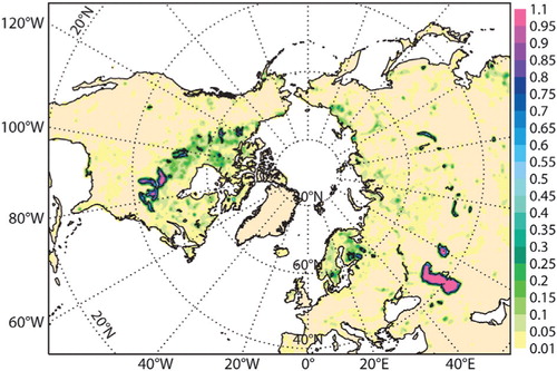
The lake cover is provided by US Department of Agriculture – Global Land Cover Characteristics (GLCC) data (Loveland et al., 2000), at a nominal resolution of 1 km. The data provide for each pixel the fraction (0–1) covered by lakes. The lake cover used in the simulations is shown in Fig. 1 for the Northern Hemisphere and for lakes that occupy more than 1% of the grid-box.

Fig. 1.  Lake cover fraction as provided by the GLCC land-cover map.

2.2.2. Lake depth.

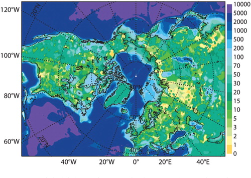
Lake depth is a crucial field controlling the water body thermal capacity, as demonstrated by several authors (e.g. Kourzeneva and Braslavsky, 2005; Balsamo et al. 2010; Dutra et al. 2010a). This variable is only available for a few lakes and it represents a real challenge for remote sensing. Additionally, lake water surfaces are not constant, and in some cases a pronounced seasonal cycle can be observed, however this is neglected in this study. A compilation of available lake depth data has been provided by Kourzeneva (2010). The processing steps to produce a global continuous field can be summarised as: (1) data were aggregated to a 5 arc-minute resolution global grid with and (2) a default value of 25 m assumed in all the inland grid points where there was no information. Moreover (3) a minimum value of 1 m was set. Although no maximum value was set at the global grid, a limit value of 60 m is presently assumed in model runs, as FLake is a shallow-water model that has no representation of the hypolimnion, a third layer usually present between the thermocline and the bottom of deep lakes. The limit value of 60 m is based on the results of Perroud et al. (2009) on the lake Geneva. The depth of the Caspian Sea was included in global map, using data from a 4 km resolution digitalised bathymetry available from Cavaleri (2008, personal communication). In addition, the Ocean bathymetry from ETOPO1 was merged to test the behaviour of the FLake model over coastal regions. It should be noted that the effect of salinity is not currently taken into account in the Flake. The resulting global bathymetry is shown in Fig. 2 for the Northern Hemisphere for all surface points (where no lakes are present or no relevant lake depth information is available, the depth is fixed to 25 m).

Fig. 2.  Global lake and oceans bathymetry (merged product described in the text).

2.3. Initial conditions for lakes

The setup of initial conditions needed to initialise the IFS deterministic forecast is normally derived from re-analysis, data assimilation or previous forecasts. However, lakes constitute a new modelling component, with a set of new prognostic variables (mixed-layer temperature and depth, bottom and average temperature, shape factor and lake ice temperature and depth).

A straightforward procedure would be to initialise the model with physically reasonable fields and allow for a long spin up (depending on the lake depth, months to years might be necessary to reach an equilibrium state). However, this is not an option due to the high computational cost of long-term atmospheric integrations. In this study, we use the initial conditions derived from a model-based climatology of lake prognostic fields. This was achieved by carrying out a long-term offline simulation of the land surface scheme forced by the ECMWF re-analysis ERA-Interim (Dee et al., 2011). This procedure has been applied and described for the offline validation of FLake within the IFS land surface component (Dutra et al., 2010a) on which the current study is based.

2.3.1. ‘Lake-planet’ experiments.

Lake simulations driven by ERA-Interim meteorological forcing have been realised with a configuration named ‘lake-planet’. This consists in assuming each surface grid-box is entirely covered by a lake with the specified lake depth from the merged bathymetry product. The advantage of this configuration is that it obtains continuous fields at the water–land interface allowing a simpler interpolation of the simulation output and independence from the lake cover dataset (which as previously mentioned can be subject to updates). The lake-planet experiment consists of a 21 yr offline run (1989–2009) of the FLake model driven by ERA-Interim 3-hourly atmospheric forcing. The ECMWF N128 Gaussian grid was adopted, which has a resolution of about 80 km. The continuity of lake-planet fields permits spatial interpolation of the model-climatology onto different target grids (e.g. a higher resolution grid), via standard bi-linear procedures. The lake-planet starts on 1 January 1989 after a 10-yr spin-up run performed on the 1989–1999 forcing, which is not used in the analysis.

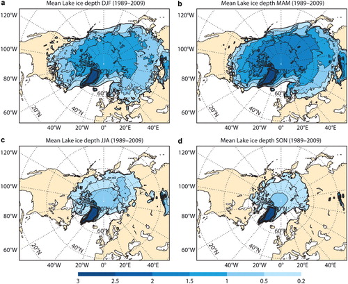
In Figs. 3 and 4 the climatology obtained is presented, respectively for the lake mixed-layer temperature and the lake ice depth. The other prognostic variables (mentioned in Section 2.1) that are needed for the lake initial conditions are taken from the same lake-planet simulations, however a direct verification is not possible, except for a very limited number of instrumented lakes.

Fig. 3.  Climatological lake mixed-layer temperature [in K] in (a) winter (DJF), (b) spring (MAM), (c) summer (JJA), (d) autumn (SON) seasons as generated by the lake-planet simulations (1989–2009).

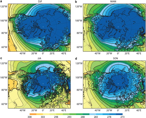
Fig. 4.  As in Fig. 3 but lake ice depth [in m].

2.3.2. Verification of lake model output.

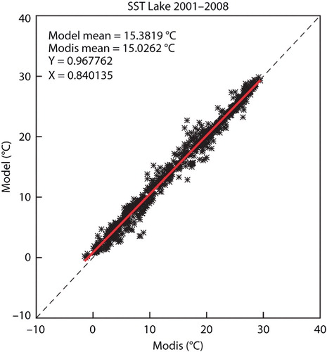
Two main verification dataset have been considered to check the accuracy of the FLake simulations. For the lake temperature, the MODIS Terra/Aqua satellite-based global composite was used. This is based on the Level 3 Mapped Thermal IR sea surface temperature (SST) product, which senses the sea/lake water surface temperature. The SST data since 2001 are available from http://oceancolor.gsfc.nasa.gov/, at a resolution of about 4 km.

The period between 2001 and 2008 is considered for validation of the simulation. The comparison between the lake-planet lake temperature simulations and the MODIS lake temperatures is shown in Fig. 5 in terms of annual mean values. Only points with more than 80% valid values in MODIS data are considered. The results indicate a largely unbiased simulation over the lakes that are considered (those occupying more than 10% of the grid-box). The largest differences between lake-planet and MODIS are found over the Caspian and the southern regions of the North-American Great Lakes (positive bias) and over Norwegian lakes (negative bias), consistently with the FLake intrinsic limitations over deep waters [not shown]. The lake temperature simulations largely reproduce, in terms of skill, the results obtained by Dutra et al. (2010a).

Fig. 5.  Comparison between the lake-planet mixed-layer temperature simulations and the MODIS LST during the period 2001–2008 over grid points where the model lake fraction is greater than 10%.

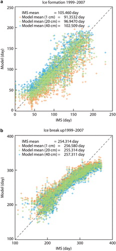
The Interactive Multisensor Snow and Ice Mapping System (IMS) (Helfrich et al., 2007) was used to validate the ice formation and break-up dates in the lake-planet simulations. The comparison of the lake-planet model output with the IMS product is provided in Fig. 6. Several ice-depth thresholds have been tested to investigate the best match to the satellite information. It should be noted that the satellite detection threshold is largely unknown. Considering an ice depth of 20 cm as detection threshold to compare with the satellite estimate (which detects only ice presence), the model shows on average an anticipation of about 9 d for the ice formation date and a delay of about 1 d for the ice break-up date. An overall 10-d bias in ice duration is comparable to errors for snow duration over land (e.g. Dutra et al., 2010b). Therefore these results are considered satisfactory given the simplified assumptions used in the ice modelling with FLake (see Mironov et al., 2010, for details on the ice scheme). However they highlight the importance of assimilating ice information for NWP operational use.

Fig. 6.  Comparison between the lake-planet ice simulation and IMS ice product: (a) ice formation day and (b) ice break-up day for three model ice-depth thresholds (1, 20 and 40 cm) are shown.

3. Forecast sensitivity experiments

Sets of 10-d forecasts covering one full year have been performed at TL399 spectral resolution (~50 km horizontal resolution) with the operational IFS (model version Cy36r3). Two experiments were performed with (LAKE) and without (NOLAKE) FLake activated. Forecasts are run 10 d apart to cover the period between the 1 January to 31 December 20081 (37 forecasts per experiment). In the NOLAKE experiment, subgrid lakes are treated as land only and resolved lakes are treated as ocean points with initial conditions (surface temperature) provided by a surface temperature monthly climatology lagged by 1 month (to represent a typical time scale of thermal inertia).

Two lakes make exception and are using near-real-time data for specifying initial conditions: the Caspian Sea, monitored by the UK Met Office SST product (OSTIA, Stark et al., 2007) and the US Great lakes, covered by the National Centers for Environmental Prediction (NCEP) daily Real-Time Global SST product (RTG, Gemmill et al., 2007).

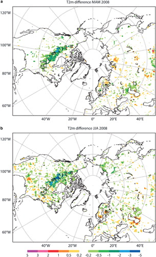
The effect of the model on near-surface temperature is evaluated for short-term (two days) forecasts. In the following discussion, the 2-m temperature (T2m) sensitivity is defined as the mean difference of LAKE compared with NOLAKE for the 48 hours forecast lead-time. Additionally, the T2m impact is defined as the Mean Absolute Error difference between the two experiment differences with respect to the IFS operational analysis. The 48 hours forecast lead-time was chosen as representative of the typical short-range NWP. The T2m sensitivity assesses the impact of the LAKE versus NOLAKE representation in IFS indicating whether a warming or a cooling is produced. On the other hand, the T2m impact evaluates the skill of forecasts when lakes are taken into account. In Fig. 7 the T2m sensitivity shows a mixture of warming and cooling signals in winter, with a similar situation in autumn. The clear autumn warming signal over Finland is very likely to be directly due to the lakes; the winter cooling signal to the East of the Great Lakes has a less obvious physical cause and is likely due to initial conditions and ice modelling. In spring and summer (Fig. 8), the cooling effect is more pronounced. This is due to the fact that the incoming radiation is stored in the lake (with a relatively small impact on surface temperature) rather than being used to warm the atmosphere. The heat stored during spring and summer (that resulted in an atmospheric cooling) is then released during autumn (leading to a warming of the near surface atmosphere). An additional cooling mechanism is that lakes can release more latent heat than dry land, resulting in lower near-surface temperatures. This is not a storage effect, and can give an overall cooling when averaged through the year. Because the results shown are simply biases after 48 hours, there is no requirement for consistency in heat balances in any case.

Fig. 7.  Sensitivity of 48-hour T2m forecasts (valid at 00 UTC) for LAKE compared with NOLAKE for (a) winter (DJF) and (b) autumn (SON). Negative values indicate cooling.

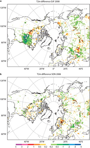
Fig. 8.  As in Fig. 7 but for (a) spring (MAM) and (b) summer (JJA).

Figures. 9 and 10 evaluate whether the temperature effects show beneficial results on the forecasts using the T2m analysis [which is based on observations from the synoptic observation report (SYNOP) and meteorological aviation report (METAR) ground based networks] as ‘ground-truth’ and calculating the Mean Absolute Error difference between the LAKE and NOLAKE forecasts. The results for winter indicate that the North American dipole highlighted by the sensitivity deteriorates the T2m temperature over central Canada while it improves in the eastern sector. This might be due to the difficulties in defining the lake ice initial conditions as illustrated in Section 3, and especially considering the choice of climatological initial conditions.

Fig. 9.  Impact of 48-hour T2m forecasts (valid at 00 UTC) for LAKE compared with NOLAKE, verified against the ECMWF T2m analysis: Mean Absolute Error difference for (a) winter (DJF) and (b) autumn (SON). Negative values indicate an improvement (MAE reduction).

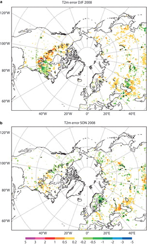
Fig. 10.  As in Fig. 9 but for (a) spring (MAM) and (b) summer (JJA).

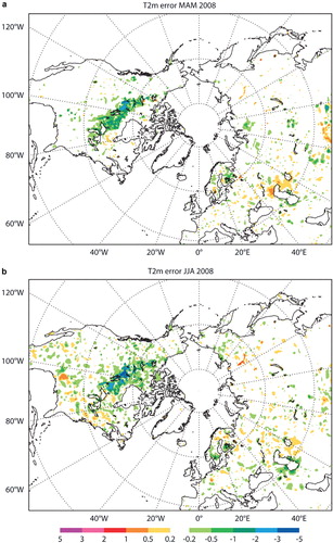
In autumn the impact is milder, however a clear improvement can be noticed over Scandinavia (with a MAE reduction between 0.5 and 1 K). A marked positive impact is obtained in spring and summer particularly over the North American lake regions and the European large lake areas. These results probably reflect the better performance of the lake model in predicting the surface temperatures in summer, comparing to winter season when lake ice predictions are controlling the impact on the atmosphere. Overall the impact is positive and shows encouraging results for future operational application also at global scale.

4. Summary and outlook

The sensitivity and impact coming from the introduction of lakes in the Integrated Forecasting System at ECMWF is analysed. Results show that the introduction of lakes in the IFS produces a delay in seasonal evolution of temperature with a cooling in spring and summer and a warming in autumn. Several preparatory steps needed to introduce this new component into the IFS are presented and discussed, particularly concerning the ancillary and the initial conditions for the new lake variables. The forecasts considering lakes–atmosphere interaction show a non-negligible signal in near-surface temperature, as a consequence of the lake thermal inertia. Winter impact is shown to be detrimental over a portion of lakes subject to freezing, most probably as a result of initial conditions errors. Near-surface temperatures in spring and summer seasons are instead largely improved, consistent with the results obtained in offline simulations.

The current analysis is limited to the thermal effects, thus dynamical aspects related to momentum or precipitation have been excluded and a more detailed analysis of the effect on the diurnal cycle should be included in future studies. The well-known winter lake effect (e.g. Laird et al., 2009) might also be improved with the adoption of interactive lakes, but the current results suggest that initial conditions will play a major role. Caveats of the current implementation are in fact mainly identified in the use of a model-based climatological initial condition, while the use of data from the correct year and, where available (e.g. Caspian Sea and US Great Lakes), the use of lake observations for both temperature and ice conditions, should be considered in future studies and for an operational implementation of lakes in the daily weather forecasts. The lake depth may also be responsible for part of the errors and an improved dataset will enhance the possibility to better simulate the lake heat storage capacity.

5. Acknowledgements

The National Snow and Ice Data Center is acknowledged for providing the IMS sea-ice cover data. We are grateful to Anton Beljaars for encouragement and helpful comments on the manuscript. Rob Hine and Anabel Bowen are acknowledged for improving figures layout. The work of Rui Salgado was partially supported by the Portuguese FCT trough project PTDC/CLI/73814/2006 and by the ECMWF.

References

- Balsamo, G, Dutra, E, Stepanenko, V. M, Viterbo, P, Miranda, P. M. A and co-authors. 2010. Deriving an effective lake depth from satellite lake surface temperature data: a feasibility study with MODIS data. Boreal Env. Res. 15(2), 178–190.
- Balsamo, G, Viterbo, P, Beljaars, A, Van den Hurk, B, Betts, A. K and co-authors. 2009. A revised hydrology for the ECMWF model: verification from field site to terrestrial water storage and impact in the Integrated Forecast System. J. Hydrometeor. 10(3), 623–643. 10.3402/tellusa.v64i0.15829.
- Dee, D. P, Uppala, S. M, Simmons, A. J, Berrisford, P, Poli, P and co-authors. 2011. The ERA-Interim reanalysis: configuration and performance of the data assimilation system. Quart. J. Roy. Meteor. Soc. 137(656), 553–597. 10.3402/tellusa.v64i0.15829.
- Dutra, E, Stepanenko, V. M, Balsamo, G, Viterbo, P, Miranda, P. M and co-authors. 2010a. An offline study of the impact of lakes on the performance of the ECMWF surface scheme. Boreal Env. Res. 15, 100–112.
- Dutra, E, Balsamo, G, Viterbo, P, Miranda, P. M. A, Beljaars, A and co-authors. 2010b. An improved snow scheme for the ECMWF land surface model: description and offline validation. J. Hydrometeor. 11(4), 899–916. 10.3402/tellusa.v64i0.15829.
- ECMWF. 2011. IFS documentation CY36r1: IV physical processes. Online at http://www.ecmwf.int/research/ifsdocs/CY36r1/index.html.
- Gemmill, W, Katz, B and Li, X. 2007. Daily real-time global sea surface temperature – high resolution analysis at NOAA/NCEP. NOAA/NWS/NCEP/MMAB Office Note Nr. 260, 39. pp.
- Helfrich S. R. McNamara D. Ramsay B. H. Baldwin T. Kasheta T. Enhancements to, and forthcoming developments in the Interactive Multisensor Snow and Ice Mapping System (IMS). Hydrol. Process. 2007; 21(12): 1576–1586.
- Kourzeneva E. External data for lake parameterization in Numerical Weather Prediction and climate modeling. Boreal Env. Res. 2010; 15: 165–177.
- Kourzeneva E and Braslavsky D. 2005. Lake model FLake, coupling with atmospheric model: first steps. In: Fourth SRNWP/HIRLAM Workshop on Surface Processes and Assimilation of Surface Variables jointly with HIRLAM Workshop on Turbulence. Workshop report, (ed. P. Unden). SMHI, Norrköping, Sweden, 43–53.
- Laird N. F. Desrochers J. Payer M. Climatology of lake-effect precipitation events over Lake Champlain. J. Appl. Meteor. Climatol. 2009; 48: 232–250.
- Loveland, T. R, Reed, B. C, Brown, J. F, Ohlen, D. O, Zhu, Z and co-authors. 2000. Development of a global land cover characteristics database and IGBP DISCover from 1 km AVHRR data. Int. J. Remote Sens. 21(6–7), 1303–1330.
- Mironov, D, Heise, E, Kourzeneva, E, Ritter, B, Schneider, N and co-authors. 2010. Implementation of the lake parameterisation scheme FLake into the numerical weather prediction model COSMO. Boreal Env. Res. 15, 218–230.
- Perroud M. Goyette S. Martynov A. Beniston M. Anneville O. Simulation of multiannual thermal profiles in deep Lake Geneva: a comparison of one-dimensional lake models. Limnol. Oceanogr. 2009; 54: 1574–1594.
- Rooney G. Jones I. D. Coupling the 1-D lake model FLake to the community land-surface model JULES. Boreal Env. Res. 2010; 15: 501–512.
- Rouse, W. R, Oswald, C. J, Binyamin, J, Spence, C, Schertzer, W. M and co-authors. 2005. The role of northern lakes in a regional energy balance. J. Hydrometeor. 6(3), 291–305.
- Salgado R. Le Moigne P. Coupling of the FLake model to the Surfex externalized surface model. Boreal Env. Res. 2010; 15: 231–244.
- Samuelsson P. Kourzeneva E. Mironov D. The impact of lakes on the European climate as simulated by a regional climate model. Boreal Env. Res. 2010; 15: 113–129.
- Stark, J. D, Donlon, C. J, Martin, M. J and McCulloch, M. E., 2007. OSTIA: an operational, high resolution, real time, global sea surface temperature analysis system. Oceans '07 IEEE Aberdeen, conference proceedings. Marine challenges: coastline to deep sea. Aberdeen, Scotland.
- Stepanenko, V. M, Goyette, S, Martynov, A, Perroud, M, Fang, X and co-authors. 2010. First steps of a Lake Model Intercomparison Project: LakeMIP. Boreal Env. Res. 15, 191–202.