Interactive lakes in the Canadian Regional Climate Model, version 5: the role of lakes in the regional climate of North America

ABSTRACT

Two one-dimensional (1-D) column lake models have been coupled interactively with a developmental version of the Canadian Regional Climate Model. Multidecadal reanalyses-driven simulations with and without lakes revealed the systematic biases of the model and the impact of lakes on the simulated North American climate.

The presence of lakes strongly influences the climate of the lake-rich region of the Canadian Shield. Due to their large thermal inertia, lakes act to dampen the diurnal and seasonal cycle of low-level air temperature. In late autumn and winter, ice-free lakes induce large sensible and latent heat fluxes, resulting in a strong enhancement of precipitation downstream of the Laurentian Great Lakes, which is referred to as the snow belt.

The FLake (FL) and Hostetler (HL) lake models perform adequately for small subgrid-scale lakes and for large resolved lakes with shallow depth, located in temperate or warm climatic regions. Both lake models exhibit specific strengths and weaknesses. For example, HL simulates too rapid spring warming and too warm surface temperature, especially in large and deep lakes; FL tends to damp the diurnal cycle of surface temperature. An adaptation of 1-D lake models might be required for an adequate simulation of large and deep lakes.

• regional climate modelling
• lake model
• coupling
• advanced surface parameterization

1. Introduction

Lakes are important components of climate system. Their influence on regional climate in continental areas, where small lakes are abundant or near large lakes, can be considerable. Accounting for lakes in modelling the climate system is essential for many regions of the world such as Northern Europe (Fennoscandian Shield) and North America (Canadian Shield and the Great Lakes area). This can be realised by interactive coupling of lake models with global and especially regional climate models. The coupling ensures that meteorological forcings provided by the atmosphere model are felt by the lake model, which in turns provides surface boundary conditions, such as surface temperature, albedo, sensible and latent heat fluxes, to the atmospheric model.

The choice of lake model formulation suitable for coupling with an atmospheric model represents certain challenges. Lake models of different degrees of complexity and based on different physical formulations exist, ranging from simple mixed-layer models to complex and computationally expensive three-dimensional (3-D) dynamical models. It is essential that lake models, when coupled with atmospheric models, should be able to reproduce adequately the behaviour of surface conditions of different lakes present within the simulation domain, while using reasonable computational time and memory resources. Thus, choosing a lake model for coupling with an atmospheric model is a matter of compromise between fidelity and computational efficiency.

One-dimensional (1-D) lake models are currently most often used for coupling with climate and Numerical Weather Prediction (NWP) models. It is also important to use appropriate lake models for different types of lakes. In typical regional model simulation domains, spanning over large parts of continents, lakes of different kinds are present, ranging from tropical lakes to temperate-zone lakes and to tundra ponds and including both small and large lakes such as the Laurentian Great Lakes in the North America, or Ladoga and Onega lakes in Eurasia. The physical processes determining the thermal regime of lakes can be different and it is possible that some lake formulations are of limited validity range and do not reproduce different lakes present in the simulation domain. In such case, using coupled-lake models may introduce additional biases into simulations, instead of removing them. For example, certain lake models do not allow for freezing the lake surface, thus making these models inappropriate for simulating annual cycles in extra-tropical regions. Testing existing lake models under different climate conditions allows to detect such situations and to facilitate the choice of lake model. A Lake Model Intercomparison Project (LakeMIP) has recently been initiated, aiming at comparing different 1-D lake models in standardised off-line simulations, corresponding to lakes of different kinds and sizes (Stepanenko et al. 2010). Knowing the validity range of different lake models would allow using different lake models for different kinds of lakes. Swayne et al. (2005) proposed using lake models of different complexity to simulate different types of lakes. Three-dimensional lake models with lake ice components were successfully applied for large lakes such as the Laurentian Great Lakes (Wang et al. 2010). Using such complex and computationally expensive models, comparable to 3-D ocean models, in an interactive coupling with climate models would require, however, fine horizontal resolution of approximately 2 km, whereas typical horizontal resolutions of existing regional climate models are of 15–50 km. Although an interactive coupling of a fine resolution 3-D lake model with a relatively coarse resolution Regional Climate Model (RCM) may be envisaged by applying some downscaling approach, it would require considerable efforts. Detailed information on lake bathymetry and geography as well as on the hydrological regime, including the inflow and outflow configuration, would also be required for running such lake models, which restricts the application of coupled 3-D lake models to a relatively small number of large lakes, for which such information is available. Given the above and the computational cost, it seems preferable to use simpler 1-D lake models, even knowing that these models lacking 3-D effects would possibly not be able to reproduce correctly enough the surface conditions of the large lakes.

In the present article, the performance of the fifth generation of the Canadian Regional Climate Model (CRCM5), coupled with two 1-D lake models, is studied, using multidecadal simulations over a domain covering the whole of North America.

The article is organised as follows: the regional climate model CRCM5, lake models and their coupling with CRCM5 are described in Section 2, the experimental setup is presented in Section 3 and the results of simulations, including the evaluation of coupled-lake models performance, the analysis of annual cycle of simulated lakes and their influence on the continental climate are discussed in Section 4. The summary is presented in Section 5.

2. Model description

2.1. Canadian Regional Climate Model

The CRCM has been developed at the University of Quebec in Montreal over the last 20 yr. This model is extensively used for climate-change simulations (e.g. Laprise et al. 1998; Laprise et al. 2003; Plummer et al. 2006; Laprise 2008). Versions 1–4 of CRCM were based on the dynamical kernel of a model initially developed by the late André Robert (see Laprise et al. 1997) with most physical parameterisations of Coupled Global Climate Model, version 2, CCGMII (McFarlane et al. 1992) and later version 3, CGCMIII (Zhang and McFarlane 1995). The fourth-generation CRCM (CRCM4; Plummer et al. 2006) is currently operational at Ouranos Consortium on Regional Climatology and Adaptation to Climate Change (De Elía and Côté 2010). CRCM4 uses the Canadian Land Surface Scheme (CLASS) version 2.7 (Verseghy 1991) that allows only one surface type (land, ocean and lake) for each grid cell. Only resolved lakes are included, either simulated by a mixed-layer model (Goyette et al. 2000) or specified from AMIP-II observation data (Kanamitsu et al. 2002) to provide lake surface temperature and lake ice fraction.

This article will employ a developmental version of the fifth-generation CRCM model (CRCM5; Zadra et al. 2008). CRCM5 is based on a limited-area version of the Global Environment Multiscale (GEM) model used for NWP at Environment Canada (Côté et al. 1998). GEM employs semi-Lagrangian transport and (quasi) fully implicit marching scheme. In its fully elastic non-hydrostatic formulation (Yeh et al. 2002), GEM uses a vertical coordinate based on hydrostatic pressure (Laprise 1992). The following GEM parameterisations are used in CRCM5: deep convection following Kain and Fritsch (1990), shallow convection based on a transient version of Kuo's (1965) scheme (Bélair et al. 2005), large-scale condensation (Sundqvist et al. 1989), correlated-K solar and terrestrial radiations (Li and Barker 2005), subgrid-scale orographic gravity-wave drag (McFarlane 1987), low-level orographic blocking (Zadra et al. 2003) and turbulent kinetic energy closure in the planetary boundary layer and vertical diffusion (Benoit et al. 1989; Delage and Girard 1992; Delage 1997). In CRCM5, however, the usual GEM land-surface scheme has been replaced by CLASS version 3.4 (Verseghy 2009) and later by version 3.5 that allows a mosaic representation of land-surface types and a flexible number of layers in the vertical position; in this article, three soil layers will be used with depths of 0.1, 0.25 and 3.75 m.

For NWP applications of GEM, lake surface temperatures and ice fraction are prescribed using climatological AMIP II data. For climate-change projections, however, such prescription is inappropriate. Lakes are often neglected altogether in global climate models, artificially changing lake grid points to land with properties of the nearest land grid point; this approach, however, is hardly tenable in RCM that purports to reproduce mesoscale processes. Hence, interactive lakes are required in RCMs.

2.2. Lake models

Two candidate formulations of 1-D thermodynamic lakes are currently being contemplated for coupling with CRCM5: the Hostetler (HL) lake model (Hostetler and Bartlein 1990; Hostetler 1991 and 1995; Hostetler et al. 1993; Bates et al. 1993 and 1995) and the FLake (FL) lake model (Mironov et al. 2010).

2.2.1. The HL lake model.

The lake model of HL solves the vertical thermal diffusion equation with a wind-driven eddy turbulence parameterised as enhanced thermal diffusion based on Henderson-Sellers (1985). The model assumes zero heat flux at the bottom of the lake. In winter conditions, when the ice insulates the lake from the atmosphere, the wind-driven mixing is absent and only molecular diffusion remains active. The model includes gravitationally driven convection, mixing the water layers once density inversion is detected. The mixed-layer depth is determined diagnostically by iterative mixing of the water surface with deep water layers until the mixed profile becomes neutral. All the incoming ultraviolet (UV) radiation and 40% of non-reflected solar (SW) radiation are absorbed at the water surface; the remaining SW radiation penetrates the water column and its absorption follows the Beer-Lambert law.

The ice and snow model is based on the modified Patterson and Hamblin (1988) formulation. The temperature within the ice/snow layers is obtained as a solution of the heat diffusion equation with the molecular diffusivity of ice/snow, taking into account the partial penetration of solar radiation into snow and ice. Ice grows when the water temperature is below the freezing point and the surface energy balance is negative. The model takes into account snow and ice melting and ablation. The snow/ice conversion processes are not taken into account. In the absence of snow or if the snow depth is below some critical minimum value (5 cm usually), the shortwave albedo is calculated using a parametric dependence on the surface air temperature. Albedo values during the wintertime are usually between 0.2 and 0.3. In the presence of a thicker snow layer, fresh snow albedo is used (0.7). The ice model allows fractional ice coverage, where a fraction of surface remains open until the ice thickness exceeds some pre-defined value (10 cm by default). Separate calculations of the water temperature profiles can be performed for open and ice-covered fractions at every time step, followed by a weighted averaging to determine the effective water temperature profile.

Because of the absence of a snow module in FL, the feature of snow on lake ice was turned off in HL for ease of comparison with FL in the simulations. However, the snow albedo was used in the HL simulations, as was also done in the FL simulations, described below.

2.2.2. The FL lake model.

The FL model is based on the concept of self-similarity of the thermal structure of the water column. This concept originates from observations of oceanic mixed-layer dynamics (Kitaigorodskii and Miropolsky 1970). A two-layered water temperature profile is assumed, with a mixed layer at the surface and a thermocline extending from the lake bottom to the base of the mixed layer. The shape of thermocline is parameterised using a fourth-order polynomial function of depth, depending on a shape coefficient C _T . A system of prognostic equations for a number of parameters, determining the thermal structure of the water column in the FL model, are described in Mironov et al. (2010). The same parametric concept is applied to the ice and snow layers, using linear shape functions, and to the bottom sediment layer; instead of the active sediment layer, the zero bottom heat flux condition can also be used. The UV radiation is absorbed at the water surface, and the non-reflected SW radiation penetrates the water column and is absorbed in accordance with the Beer-Lambert law. A system of prognostic ordinary differential equations is solved for the thermocline shape coefficient, the mixed-layer depth, bottom and surface water temperatures, shape parameter and temperature of the active sediment layer as well as ice and snow temperatures. The mixed-layer depth equation includes convective entrainment, wind-driven mixing and volumetric solar radiation absorption. The two-layer water temperature parameterisation of the FL model limits its applicability in the case of deep lakes because it does not allow for the hypolimnion layer between the thermocline and the lake bottom. Consequently, in such cases, a ‘virtual bottom’, usually at 40–60 m, is used in simulations instead of the actual lake depth. The parametric structure of the FL model does not allow for partial ice coverage, as in HL's model. The snow module is optional in the FL model; however, its use is not yet recommended by the mode developers. Instead, a correction of the ice albedo, taking into account the influence of the snow cover, is applied; its value is usually between 0.2 and 0.3.

2.3. Coupling of CRCM5 with lake models

The mosaic approach of CLASS 3.5 allows for co-existence of multiple surface types in each model grid cell. The currently allowable surface types are: (1) land calculated by CLASS, (2) ocean – either open water or ice – currently prescribed from AMIP II climatological data, (3) ice sheets and (4) urban areas. A new surface type, corresponding to land water bodies or lakes, has been added for the CRCM5 model. In the mosaic approach, the same fields are seen by all the surface types within a given grid cell; this includes atmospheric variables such as surface air pressure, screen-level air temperature and moisture and anemometer-level winds and derived fields such as downward solar and terrestrial radiation fluxes at the surface and precipitation. For each surface type, separate calculations are performed for surface thermal emission and fluxes of heat, moisture and momentum; these fields and others such as surface temperature and albedo are then aggregated, weighted by their respective areal fraction, and the resulting values returned as lower boundary condition to the atmospheric column. In fact, over lakes, latent and sensible heat fluxes are calculated separately for both open-water and ice-covered parts of simulated lakes.

3. Experiment setup

A 50-year long (1958–2007) simulation was performed over a domain, covering the North American continent and neighbouring oceans and islands, consisting of 170×158 grid points on a rotated latitude–longitude grid, with horizontal grid spacing of 0.5°, as shown in Fig. 1. Twenty grid points around the perimeter of the domain are used for nesting; the outermost 10 grid points serve as ‘halo’ for providing upstream data in the semi-Lagrangian interpolation, and the next 10 grid point ribbon serves as Davies sponge where CRCM atmospheric variables are damped towards the driving fields. This leaves a free innermost domain of 130×118 grid points. The atmospheric model used 56 layers in the vertical and a time step of 20 m. The model was driven by ERA40 reanalysis from 1958 until August 2002 and by the ERA-Interim reanalysis from September 2002 until 2007. AMIP II data were used for prescribing ocean surface temperatures and ice cover fraction.

Fig. 1.  The entire simulation domain comprising 170×158 grid points, and the outer 20 grid point halo and nesting zones. The lake fraction (in%) and lake depths (m) are shown. The blue arrows show locations of lakes used for evaluation of simulations and presented in Figs 2–13 and Table 1. The dashed contour denotes the lake-rich region of the domain, shown in Figs 14–19.

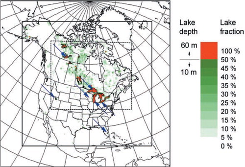
The lake fraction values used in simulations are also shown in Fig. 1. Except for the largest lakes, lake depths are generally not available. In the absence of available detailed data for lake depths, the following simple lake depth parameterisation was used: 60 m if the lake fraction exceeds 50% and 10 m otherwise, as shown in Fig. 1. This lake depth parameterisation is based on the assumption of shallowness of small lakes, as in Samuelsson et al. (2010), and on the results of lake model sensitivity studies (Martynov et al. 2010) that show the insensitivity of the HL lake model on the lake depths exceeding 40 m and the maximum lake depth recommended by FL model authors (Mironov et al. 2010). An additional FL-coupled CRCM5 simulation has been performed using the global lake depth database developed by Kourzeneva (2009); this simulation has been used for comparison of coupled-lake model performance in the lake Erie. One-meter-thick vertical layers were used in the HL model. A lake water transparency of 0.2 m⁻¹ was used for the whole domain. Three simulations were performed: a ‘no-lake’ (NL) simulation in which lake grid cells were substituted by adjacent land-surface types or by a linear interpolation of nearby cell land proprieties (land-surface types and their relative fractions) in the case of 100% lake coverage; HL using the HL model for inland waters; and FL using the FL model for inland waters.

For evaluation of the simulations, a number of lake sites were selected, representing lakes of different mixing regimes, depths and sizes, located in different climatic zones. Lake sites, their characteristics and available data sources are presented in Table 1.

Table 1. Lake evaluation sites: characteristics and data sources

Lake name	Lake type, geographical location	Lake surface/fraction	Lake depth: real average/ simulated	Data type, coordinates, data source
Great Slave Lake, Northwest Territories	Large deep northern freshwater lake	27 200 km^2 100%, several tiles	42/60 m	MODIS-derived daily-averaged SST values (61.37N, 114.82W) (H. Kheyrollah Pour, personal communication)
Lake Superior	Large deep temperate freshwater lake	82 400 km^2 100%, several tiles	147/60 m	NDBC buoy 45001 (48.06N, 87.78W)
Lake Michigan	Large deep temperate freshwater lake	58 000 km^2 100%, several tiles	85/60 m	NDBC buoy 45007 (42.70N, 86.97W)
Lake Erie	Large shallow temperate freshwater lake	25 774 km^2 100%, several tiles	19/60 m/20 m (in the realistic depth parameterisation CRCM5-FLake run, ‘FL-depth’)	NDBC buoy 45005 (41.68N, 82.40W)
Sparkling Lake, Wisconsin	Small shallow temperate freshwater lake	0.64 km^2 8% (together with other lakes)	11/10 m	NTL LTER project buoy (46.01N, 89.7W)
Great Salt Lake, Utah	Medium-sized shallow salt lake	4400 km^2 49.7%	4.9/10 m	US Geological Survey gauging stations 1001000 (40.73N, 112.21W) and 10010100 (41.26N, 112.50W)
Lake Okeechobee, Florida	Medium-sized shallow freshwater lake	1900 km^2 43%	2.7/10 m	Southwest Florida Water Management District station LZ40 (21.90N, 80.79W)

4. Results

4.1. Evaluation of CRCM5 with interactive lakes

Lake surface temperature is one of the most important parameters affecting the interactions between the atmosphere and the lakes, and hence a detailed comparison of simulated lake surface temperatures with observations has been performed for seven lakes of different mixing regimes, depths and sizes, located as shown in Fig. 1 in different climate zones of the North American continent. Figures. 2 3 4 5 6 7 8 show daily-averaged lake surface temperatures for HL and FL simulations, compared with instantaneous or daily-averaged observations of different types and sources. The evaluation period is chosen differently for the lakes based on the availability and quality of observation data.

Fig. 2.  Comparison of simulated lake surface temperatures with MODIS-derived values for Great Slave Lake, Northwest Territories.

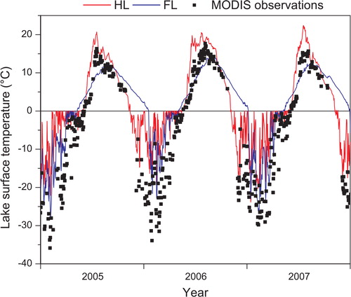
Fig. 3.  Comparison of simulated lake surface temperatures with buoy observations for Lake Superior.

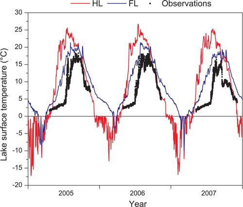
Fig. 4.  Same as Fig. 3, but for Lake Michigan.

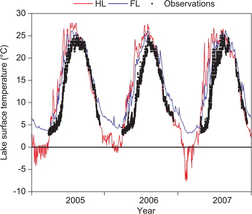
Fig. 5.  Same as Fig. 3, but for Lake Erie. FL-depth: simulated lake surface temperature, obtained with realistic lake depth parameterisation (20 m at the lake Erie buoy location).

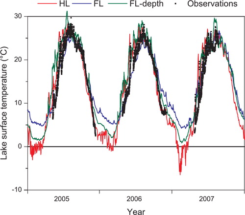
Fig. 6.  Same as Fig. 3, but for Sparkling lake, Wisconsin.

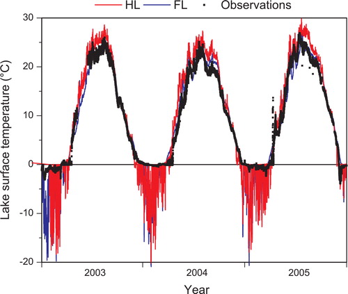
Fig. 7.  Same as Fig. 3, but for Great Salt Lake, Utah.

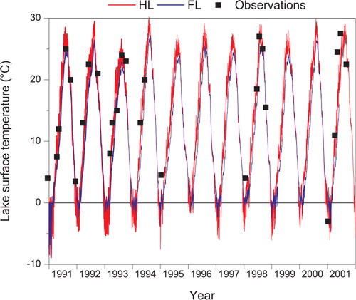
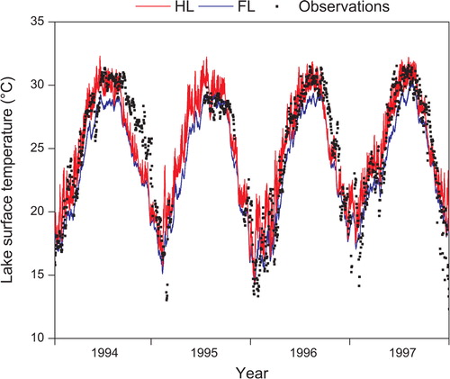
Fig. 8.  Same as Fig. 3, but for Lake Okeechobee, Florida.

4.1.1. Great Slave Lake.

Great Slave Lake is a large and deep northern lake. It is a dimictic freezing lake, covered by ice during a substantial part of the year. The daily-averaged moderate resolution imaging spectroradiometer (MODIS)-derived observation values (H. Kheyrollah Pour, personal communication) and simulated surface temperature data corresponding to the central basin of the lake are shown in Fig. 2. It can be seen that the annual pattern of the lake surface temperature is generally well reproduced by HL and FL simulations. Minimum winter ice surface temperatures are fairly close to observations for both simulations. The ice-off date is best reproduced by HL, with FL being too early. This might be caused by the absence of thermal insulation of the snow cover in FL-coupled simulations, as it was shown that the presence or absence of snow on ice might influence the ice-off date (Dutra et al. 2010). However, HL produces an excessively rapid spring warming caused by unrealistically warm water temperature profile under the ice in wintertime, which is a documented feature of this model (e.g. Martynov et al. 2010). FL reproduces well the observed characteristic slow warming in spring and summer, and slow cooling in autumn, although it produces a later freezing up than it is observed.

4.1.2. Lake Superior.

Lake Superior is the largest and deepest freshwater lake of North America. Several American and Canadian meteorological buoys are placed on the lake in the open-water periods, providing regular surface water temperature observations. The data, collected by the NDBC buoy 45001, located in the central part of the lake, are presented in Fig. 3, along with simulated values. Lake Superior is characterised by a very slow spring warming, lasting till the surface temperature exceeds 4 °C. The HL simulation produces excessively rapid spring warming and exceedingly high summer temperatures, up to 8 °C warmer than in observations. The simulated temperatures reach their highest values much earlier than observed and begin to decline when in fact the observed peak occurs. The spring warming with FL is also somewhat too rapid and maximum summer temperatures are too high by ~4 °C. FL also simulates later and slower autumn cooling than observed, and much shorter ice-covered periods.

4.1.3. Lake Michigan.

For the southern part of Lake Michigan (Fig. 4), the simulation results are much closer to the observations (NDBC buoy 45007) than in the case of Lake Superior. Both lake models produce slightly earlier spring warming than observations and the simulated maximum temperatures are higher than observed by ~5 °C with HL and ~2–3 °C with FL. In autumn, HL reproduces well the observed temperatures, and in winter, it produces relatively long ice-covered period. FL produces slightly delayed cooling in autumn; in winter, however, the surface temperatures are too high and the lake remains ice free.

4.1.4. Lake Erie.

Lake Erie is the shallowest of all the Great Lakes, with an average depth of 19 m. According to the simple depth parameterisation employed, based on the lake fraction, this lake was simulated using an excessive depth of 60 m. The comparison of simulated surface temperature with the NDBC buoy 45005 is presented in Fig. 5. As for Lake Michigan, there is good agreement between simulated and observed surface temperatures in summertime. With FL, the autumn cooling is somewhat too slow, wintertime temperatures are too warm and the lake remains ice free. The underperformance of the FL model for lake Erie may result from using an excessive depth for this lake, as the autumn cooling becomes longer with increasing lake depth, whereas the performance of the HL model depends only weakly on the lake depth (Martynov et al. 2010). Applying more realistic lake depth parameterisation, such as that proposed by Kourzeneva (2009) improves the performance of the coupled model. Figure 5 shows that using a realistic lake depth (20 m in the Lake Erie buoy location), the FL-simulated autumn cooling becomes much faster with a depth of 60 m and better reproduces the observed surface temperatures. Note that, the FL winter temperatures are still higher than those in the HL case.

4.1.5. Sparkling Lake.

Sparkling Lake is a small and shallow temperate-forest lake, located in Wisconsin, near the lakes Superior and Michigan. On the corresponding grid, the lake fraction is around 8%, which accounts for numerous subgrid lakes of the region. Multiannual observations of this lake were carried out by the NTL LTER project, directed by the University of Wisconsin. The buoy observations, obtained from the NTL LTER project, are compared with simulations in Fig. 6. The FL-simulated lake surface temperatures follow well the observed open-water temperatures, whereas the HL predicts slightly earlier and faster spring warming, with maximum temperatures ~3 °C warmer than observed. The ice-covered periods are well reproduced by both lake models; during these periods the observations correspond to the temperature of under-ice water, hence close to the freezing point.

4.1.6. Great Salt Lake.

The Great Salt Lake in Utah is a large shallow salt lake, located in an area with dry arid climate. Both lake models, coupled with CRCM5, were run under the assumption of freshwater, so the relation of simulations with lake measurements represents a certain interest. Some observations were carried out on two lake-level measurement stations of the US Geology Survey, and these are compared with simulated surface temperatures in Fig. 7. Both coupled-lake simulations match fairly well with the scarce available observations of surface temperatures. The HL produces slightly higher maximum temperatures that FL. In winter periods, both models predict freezing of the lake. However, it is known that because of extremely high concentration of minerals (near 16%), the Great Salt Lake does not freeze, which in fact causes locally significant lake-effect precipitations in winter (Steenburgh et al. 2000).

4.1.7. Lake Okeechobee.

Lake Okeechobee is a large shallow freshwater lake, located in the tropical climate area of Southern Florida. The meteorological buoy LZ40 of the Southwest Florida Water Management District (SFWMD) is permanently placed near the centre of the lake. Water surface temperature measurements from this buoy are presented in Fig. 8 along with simulated values. There is a good agreement between coupled-lake simulations and observations. As in previous cases, the HL temperatures are slightly higher in spring and in summer than those produced by FL, whereas in autumn and winter both models produce similar results.

4.2. Average annual cycle at lake evaluation sites

Although lake surface temperature is a very important variable, it is not the only variable to couple the surface with the overlaying atmosphere. It is important to verify that the surface processes are correctly reproduced in the coupled system. A comparison of coupled-lake simulations with the NL case can serve to highlight important surface processes occurring in lake-rich regions. For this purpose, Figs 9 10 11 12 13 show the average annual cycles over the 30-year period 1973–2002, for the NL and the two coupled-lake (HL and FL) simulations, for the following fields: surface and screen-level air temperature, surface and screen-level air specific and relative humidity and sensible and latent heat fluxes. Surface specific humidity is defined as the saturation values corresponding to surface temperature in the presence of lakes. For temperature and specific humidity, the figures show the screen-level air values and the difference between surface and the screen-level air values to highlight the surface layer gradients. For sensible and latent heat fluxes, the figures show the simulated values for the NL case and the differences between the coupled-lake and NL simulations to highlight the effect of lakes. The screen-level temperature and specific humidity values correspond to tile averages. Surface values and surface heat fluxes are shown for the lake surface type in the HL and FL simulations and for land in the NL case.

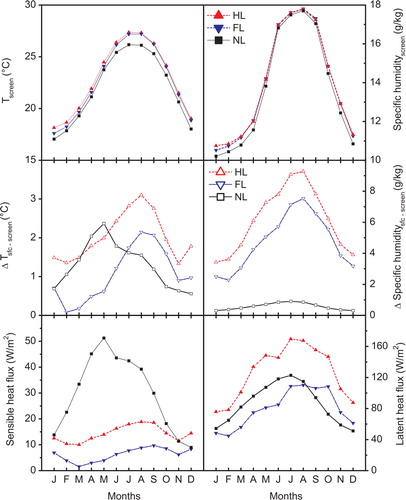
Fig. 9.  Annual cycle of simulated fields for Great Slave Lake, by the no-lake (NL) and the two coupled-lake (HL and FL) simulations, averaged over the 30-year period 1973–2002. The following fields are shown: screen-level temperature (upper left panel, in °C), screen-level specific humidity (upper right panel, in g kg⁻¹), difference between the surface and screen-level air temperatures (middle left panel, in °C), difference between the surface and screen-level specific humidity (middle right panel, in g kg⁻¹), surface sensible heat fluxes (lower left panel, in W m⁻²) and surface latent heat fluxes (lower left panel, in W m⁻²). Solid symbols denote absolute values, open symbols – differences.

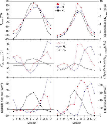
Fig. 10.  Same as Fig. 9, but for Lake Superior.

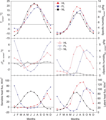
Fig. 11.  Same as Fig. 9, but for Lake Sparkling.

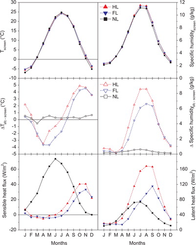
Fig. 12.  Same as Fig. 9, but for Great Salt Lake.

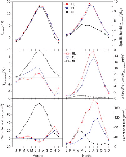
Fig. 13.  Same as Fig. 9, but for Lake Okeechobee.

Figures 9 10 11 12 13 show the comparison for five of the earlier employed lake sites; the case of the Great Slave Lake is analysed in details, whereas for other lakes the most important features of their annual cycles will be described.

4.2.1. Great Slave Lake.

The average annual cycles for Great Slave Lake are presented in Fig. 9. The screen-level air temperature is lower in summer and higher in winter with coupled lakes compared to the NL simulation, as is to be expected. The difference between the surface and the screen-level temperature is enhanced with coupled lakes compared to the NL simulation. The sign of the difference reverses between summer and winter, and that sign is opposite in the coupled simulation compared to the NL case. In the NL simulation, the difference is positive in summer and negative in winter. The unstable conditions in summer reflect the fact that the land surface is heated by absorbed solar flux, leading to an unstable boundary layer; in winter on the other hand, the surface is cooled by terrestrial radiation under predominantly clear sky conditions, leading to stable boundary layer. In the coupled-lake simulations, the surface air temperatures are cooler in summer and warmer in winter, demonstrating the thermal damping induced by large lakes. In spring and summer, the differences between the surface and the screen-level temperature are negative in coupled-lake simulations; in spring this is because of the slower warming of lakes when the stratification is being developed in lakes and in summer this is due to wind-induced mixing that forms the relatively cool mixed layer in lakes. Thus, during this period the surface conditions over Great Slave Lake remain stable. The destabilising change of the temperature difference to positive values occurs earlier in the HL-coupled simulations and is evidently linked to relatively fast spring warming and high maximum temperatures produced by this model (Fig. 2). In the cases of FL, this change occurs much later and is associated with autumn cooling of the atmosphere and the large thermal inertia of the lake. In both coupled-lake simulations, the surface layer becomes unstable in autumn and remains unstable during wintertime. Relatively slow autumn cooling in the FL case is associated with maximum temperature difference of ~9 °C reached in November, when the screen-level temperatures are already below freezing, but the lake is still not frozen with FL (Fig. 2).

The average annual cycle of specific humidity is similar in all simulations, including NL, but HL and FL simulations reach peak values later in summer compared to NL. The highest summer values were obtained in the HL simulations. The differences between the surface and screen-level specific humidity are markedly different in the coupled-lake and NL cases. In the NL case, the differences are small and positive in summer and almost disappear in winter, whereas they are much stronger in coupled-lake simulations, reaching their minimum in spring and early summer, increasing importantly in autumn and winter periods. This can be explained by the role of the surface-layer stability that suppresses evaporation in spring and early summer.

The annual cycle of the surface sensible heat flux shows a strong difference between the coupled-lake and NL cases: the NL sensible heat flux reaches maximum values in summer months, whereas coupled-lake values are close to zero or negative in this period. In autumn and winter, however, the situation changes: the NL sensible heat becomes negative; whereas, with coupled lakes, the sensible heat flux becomes positive and strong. This agrees well with the earlier discussed surface-layer stability conditions. In the absence of lakes, warm land surface causes strong sensible heat flux in summer, but in the coupled-lake cases, the surface conditions are stable, with air temperature warmer than the lake surface, which results in weak negative sensible heat fluxes. The thermal inertia of lakes leads to the formation of unstable surface conditions and strong sensible heat flux during the autumn cooling period. In the NL case, the surface is rapidly cooling, leading to weak positive sensible heat flux values. In wintertime, the coupled-lake sensible heat flux remains positive, whereas in the NL winter sensible heat flux is negative due to strong radiative cooling of the land surface.

The maximum NL latent heat flux is obtained in the spring and summer periods, whereas it is close to zero in coupled-lake cases. The coupled-lake flux becomes positive and strong in the late summer and in autumn because of unstable surface conditions. In winter, the latent heat flux is weak in all cases because of very low surface temperatures.

Our results obtained for Great Slave Lake are in good agreement with those obtained by Long et al. (2007) with the 3-D dynamical POM lake model. This lends some confidence in the appropriateness of the chosen 1-D framework for coupled lakes in CRCM5 model.

4.2.2. Other lakes.

The mean annual cycle of variables for Lake Superior are presented in Fig. 10. There are no substantial differences between this lake and Great Slave Lake, once taking into account the different climate conditions and geographical location. Both lakes are large and deep dimictic freezing lakes, resolved at the current horizontal resolution of CRCM5 (0.5°) and covering entirely several model grid tiles.

Sparkling Lake, shown in Fig. 11, is quite different from both previous cases by being a small and shallow subgrid lake, with 8% of lakes on the grid tile. In such conditions, the screen-level air temperature and humidity are mostly determined not by lakes but by adjacent land that covers the remaining 92% of the tile. It can be seen that the presence of lakes leads to similar differences from the NL case as in large resolved lakes, although to a much lesser extent. The screen-level air temperature is slightly lower in summer and slightly higher in autumn in coupled-lake simulations than in the NL case, whereas the tile-averaged surface specific humidity is higher in coupled-lake simulations than in the NL cases. This can be explained by the shallow depth of temperate subgrid lakes, resulting in rapid heating of lake water column, which leads to earlier evaporation onset, compared to deep and cold Great Lakes.

The Great Salt Lake mean annual cycle is presented in Fig. 12. This lake is large and occupies nearly 50% of two adjacent simulation grid tiles. Thus, the influence of this lake on the air temperature and humidity should be more important than that of Sparkling Lake. The screen-level air temperatures are fairly similar in all simulations. The air humidity depends strongly on the presence and simulation regime of lakes. Lying in an arid climate region, the air in the NL case is substantially drier than in coupled-lake cases at comparable temperatures. In the presence of lakes, the screen-level air humidity generally follows the temperatures and surface layer stability (Figs 7 and 12): maximum for the HL, slightly less in the case of FL.

The annual cycle of the tropical Lake Okeechobee is presented in Fig. 13. The screen-level air temperatures in coupled-lake simulations exceed those in NL during the entire year; in fact the boundary layer remains unstable in all simulations during the whole year. The surface temperature in coupled-lake simulations is higher than in the NL one, possibly due to the lower surface albedo combined with shallowness of the lake. The screen-level specific humidity is similar in all simulations, with the coupled-lake simulations being slightly higher than those of the NL case; nevertheless, the surface specific humidity is high in absence of lakes in these wet tropical climate conditions. High positive temperature and humidity differences between the surface and the screen level indicate strong latent and sensible heat fluxes in all simulations; these fluxes are smaller for the FL case, resulting in lower surface temperatures, closer to the screen-level values.

4.3. Continental climate in coupled lake and ‘no lake’ simulations

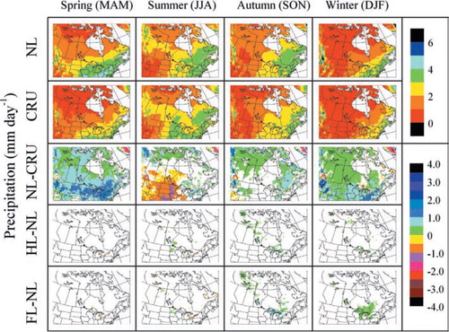
In this section, we will look at seasonal mean maps, averaged over the 30-year period 1973–2002. The seasonal averages of the screen-level temperature, screen-level specific and relative humidity, surface sensible and latent heat fluxes and precipitation are shown in Figs 14 15 16 17 18 19 . Maps are shown for four seasons, defined as 3-month averages: spring (MAM), summer (JJA), autumn (SON) and winter (DJF). Most figures show (1) the NL simulation, (2) a corresponding observational or analysis verification (CRU or ERA) dataset, when available, (3) the NL simulation bias calculated as the difference between the NL simulation and the reference, when available, (4) the difference between the HL and NL simulations and (5) the difference between the FL and NL simulations. These last two set of figures will serve to highlight the influence of lakes on the simulated climate of North America; the difference maps will only show values where the differences are statistically significant. The statistical significance of differences was estimated by comparing the coupled lake and NL differences to the interannual variability of monthly averages for the 30-year period. The statistical significance was calculated by implementing a two-sided Student t-test with α=5%.

Fig. 14.  Screen-level temperature (in °C) climatological maps for 1973–2002, by ‘seasons’: spring (MAM), summer (Summer (JJA)), autumn (Autumn (SON)) and winter (Winter (DJF)). Top row corresponds to the NL simulation, second row to the reference CRU gridded analysis of observations, third row to the NL-simulation bias calculated as the difference between the NL simulation and the reference, fourth row to the difference between the HL and NL simulations and fifth row to the difference between the FL and NL simulations. Results are only shown over the continent, and the differences are only shown where statistically significant at the 95% level.

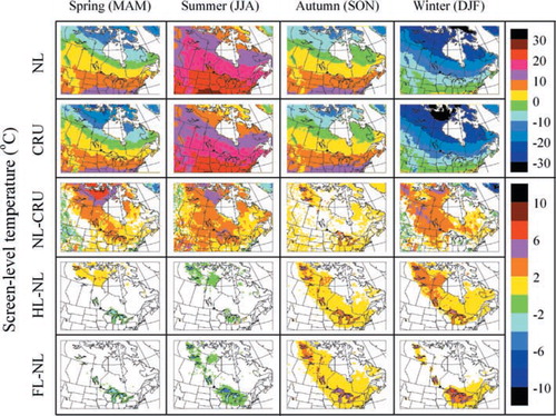
Fig. 15.  Climatological maps for 1973–2002 of screen-level specific humidity (in g kg⁻¹). Top row corresponds to the NL simulation, second row to the difference between the HL and NL simulations and third row to the difference between the FL and NL simulations. Results are only shown over the continent and where the differences are statistically significant at the 95% level.

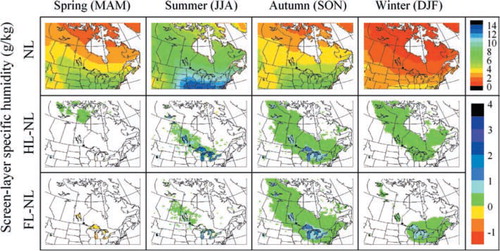
Fig. 16.  Same as Fig. 15, but for relative humidity (in%).

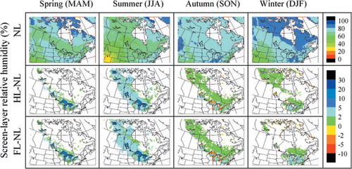
Fig. 17.  Same as Fig. 15, but for surface sensible heat flux (in W m⁻²). In this case, the ERA40 data are used as reference.

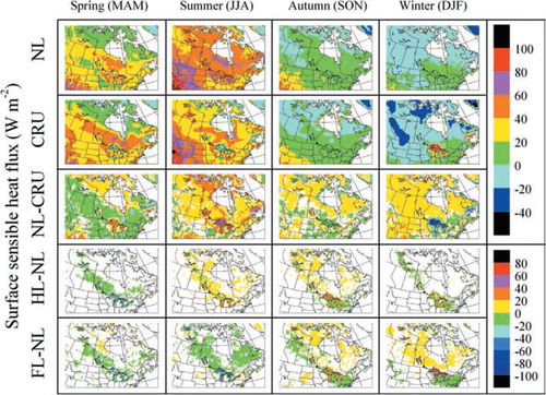
Fig. 18.  Same as Fig. 17, but for surface latent heat flux (in W m⁻²).

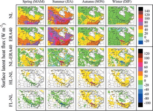
Fig. 19.  Same as Fig. 15, but for precipitation (in mm day⁻¹).

As the influence of lakes is felt predominantly in the lake-rich regions, from the Great Lakes through the Canadian Shield, up to the Great Bear Lake, only this region will be presented in Figs 14 15 16 17 18 19 .

Screen-level temperature maps show a warm bias in the NL simulation for all seasons. This early version of CRCM5 has by now been documented as suffering from a strong warm and dry bias over continents, especially in summer, as a consequence of the non-water conserving formulation of the shallow convection scheme. Precipitation deficits are accompanied by a deficit of clouds, which results in excess solar heating and drying of the surface and excess ratio of sensible over latent surface heat flux. This defect has been corrected in subsequent versions of the model, but it must be kept in mind that the simulations presented in this article do suffer from this documented bias. Nonetheless, we will proceed with the analysis of the impact of coupled lakes on the simulated results by focusing on the differences between the HL and FL coupled-lake simulations and the NL one.

As discussed earlier, the damping effect of lakes on coupled-lake simulations is clearly seen in Fig. 14, with lower screen-level temperatures in spring and summer and higher temperatures in fall and winter, over large lakes and in the vicinity of regions with abundant lakes. Over the Great Lakes, the lake surface temperature decreases faster in autumn in the HL simulation compared to FL. It results in a reduction of the warm bias over the NL temperature in the HL case, compared to the FL case. As it was seen earlier, this results in longer ice-covered periods and, correspondingly, lower surface temperatures in winter than the FL simulation. However, in northern lakes HL produces higher fall and winter temperatures than FL. This might be caused by additional heat flux through the ice cover, which is not thermally insulated by the snow layer, in the presence of relatively warm water at 4 °C directly under the ice cover and a thin temperature gradient layer, formed in the HL simulations in the absence of wind-driven vertical water mixing (Martynov et al. 2010). This mechanism, which seems inadequate for Northern lakes, can explain the formation of the large warm area in the northwestern part of the Canadian Shield in HL simulations. In the cases of FL, the influence of lakes on the screen-level temperature is statistically significant over the large lakes and in the close vicinity of the Great Lakes, where the warming effect can reach 4 °C. There is no statistically significant effect of lakes on subgrid lake regions of the Canadian Shield, away from the Great Lakes.

It can be seen in Figs 15 and 16 that, in spring, the coupling with lakes results in reduced specific humidity but increased relative humidity over lakes, as a result of lower temperatures there; as is to be expected, exactly the reverse is noted in autumn. In winter, specific and relative humidity are increased over the Laurentian Great Lakes and in their vicinity, up to distances of 200–300 km with FL and smaller distances with HL. Over northern lakes, however, HL produces a larger increase in humidity than FL, in agreement with the temperature patterns described earlier.

Figure 17 shows that the presence of lakes reduces surface-sensible heat flux in spring and summer over lakes and regions with abundant subgrid lakes, due to the cooler lake surface compared to land; the reverse is of course noted in fall and winter, especially with FL.

Figure 18 shows that overall latent heat flux is affected in a similar fashion as sensible heat flux. However, there is an exception: a slight reduction of latent heat flux is noted downstream of the Great Lakes in winter, probably due to the increased atmospheric moisture there, as a result of the increased evaporation rate over the lakes. Also the increased latent heat flux over the Great Lakes is most marked in autumn, whereas the increased sensible heat flux was larger in winter.

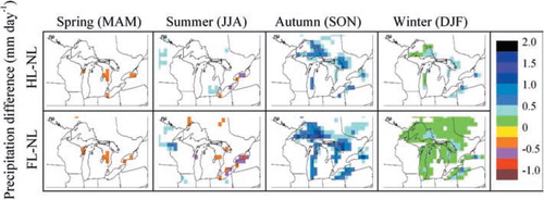
In Fig. 19, we note a decrease (increase) in precipitation downstream of the lakes in spring and summer (autumn and winter). The increase in autumn and winter corresponds to the model attempting to simulate snow squalls that are prevalent during cold outbreaks downstream of major open-water surfaces. These regions that are referred locally as snow belts can receive annually snow amounts up to 3.5 m. Figure 20 shows a blow up of the precipitation differences with coupled lakes in the regions of the Great Lakes. It is seen that the precipitation increase spans a distance of 1–3 grid points downstream of the lakes. With a 0.5-grid, however, clearly the model does not have the resolution to adequately resolve snow squalls as they occur in nature.

Fig. 20.  Blow up over the Great Lakes region of the precipitation differences (in mm day⁻¹), displayed on the bottom two rows of Fig. 19.

5. Summary and conclusions

An interactive coupling of the CRCM5 with 1-D column lake models has been realised. Multidecadal simulations of the climate of North America were performed with two different lake formulations, HL model and FL model and were compared to a simulation without lakes (NL) and with available observations.

A detailed comparison of simulated lake surface temperatures was made with those observed at seven lake sites located in different climatic zones of the continent. Interactive lake models have demonstrated a good performance in temperate subgrid lakes and in large shallow lakes, located in the arid (Great Slave Lake) and tropical (Lake Okeechobee) climate. For these lakes, FL performed best, as HL tended to overestimate the lake surface temperatures, especially in large and deep lakes.

Large and deep lakes constitute a challenge for 1-D thermodynamic column lake models, as it has been shown in offline simulations (Martynov et al. 2010) and confirmed in coupled simulations, presented in this article. The relatively poor performance of 1-D lake models, particularly for large deep lakes, is essentially due to the lack of representation of 3-D processes such as upwelling and downwelling, mixing caused by horizontal currents and thermal bar formation. The performance of 1-D models could in principle be improved by adapting the physical parameterisation of 1-D models, based on empirical data or on 3-D simulations. Implementation of 3-D lake models, interactively coupled with regional climate models, can be envisaged as a potentially more physically adequate and reliable solution, albeit a computationally costly one.

An important issue is that the 1-D lake models, ignoring 3-D mixing processes, seem to underestimate the total heat storage capacity of large and deep lakes, which leads to biases in the thermodynamic balance and feedbacks between lakes and atmosphere. This is particularly true with the HL model where, as it has been shown by Martynov et al. (2010), the mixed-layer depth does not depend substantially on the lake depth for intermediate and deep lakes. The FL model reproduces better the deepening of the mixed layer with the lake depth, but the artificial limitation of the effective lake depth, at 60 m in the present work, which is necessary for this model, limits its ability to adequately reproduce deeper lakes. Using realistic lake depth parameterisation improves the performance of coupled simulations on large shallow lakes in the case of the FL model.

The presence of lakes influences mostly the lake-rich region of the Canadian Shield by altering the low-level air temperature, humidity and precipitation. The influence of lakes on the precipitation is most significant over the Laurentian Great Lakes and within the distance of 200–300 km downstream of these lakes, especially with open water on lakes in wintertime. The patterns of enhanced precipitation correspond to regions of the well-known lake effect snow on downwind coasts of the Great Lakes. The influence of lakes on air temperature and humidity in subgrid lake-rich regions of the continent is weak in FL simulations. The warming effect produced by the HL in winter in the northwestern part of the Canadian Shield results in exaggerated heat flux from the water through the ice cover in the absence of insulating snow layer, produced by this lake model.

6. Data sources and credits

ERA40 reanalysis: Uppala, S. M., Kållberg, P. W., Simmons, A. J., Andrae, U., da Costa Bechtold, V., Fiorino, M., Gibson, J. K., Haseler, J., Hernandez, A., Kelly, G. A., Li, X., Onogi, K., Saarinen, S., Sokka, N., Allan, R. P., Andersson, E., Arpe, K., Balmaseda, M. A., Beljaars, A. C. M., van de Berg, L., Bidlot, J., Bormann, N., Caires, S., Chevallier, F., Dethof, A., Dragosavac, M., Fisher, M., Fuentes, M., Hagemann, S., Hólm, E., Hoskins, B. J., Isaksen, L., Janssen, P. A. E. M., Jenne, R., McNally, A. P., Mahfouf, J.-F., Morcrette, J.-J., Rayner, N. A., Saunders, R. W., Simon, P., Sterl, A., Trenberth, K. E., Untch, A., Vasiljevic, D., Viterbo, P. and Woollen, J. 2005: The ERA-40 re-analysis. Q J R Meteorol Soc. 131, 2961–3012. DOI: 10.1256/qj.04.176.

ERA-Interim reanalysis: Dee, D. P., Uppala, S. M., Simmons, A. J., Berrisford, P., Poli, P., Kobayashi, S., Andrae, U., Balmaseda, M. A., Balsamo, G., Bauer, P., Bechtold, P., Beljaars, A. C. M., van de Berg, L., Bidlot, J., Bormann, N., Delsol, C., Dragani, R., Fuentes, M., Geer, A. J., Haimberger, L., Healy, S. B., Hersbach, H., Hólm, E. V., Isaksen, L., Kållberg, P., Köhler, M., Matricardi, M., McNally, A. P., Monge-Sanz, B. M., Morcrette, J.-J., Park, B.-K., Peubey, C., de Rosnay, P., Tavolato, C., Thépaut, J.-N. and Vitart, F. (2011), The ERA-Interim reanalysis: configuration and performance of the data assimilation system. Q J R Meteorol Soc. 137, 553–597 DOI: 10.1002/qj.828.

CRU climate data: Mitchell, T. D, Jones, 2005. An improved method of constructing a database of monthly climate observations and associated high-resolution grids. Int J Climatol. 25, 693–712 DOI: 10.1002/joc.1181.

Great Slave Lake: MODIS-based data, treated by H. Kheyrollah Pour, University of Waterloo, Ontario, Canada (personal communication). MODIS raw data source: NASA Land Processes Distributed Active Archive Center (LP DAAC)

Great Lakes observation buoys: National Data Buoy Center (NDBC), NOAA, US. Department of Commerce.

Sparkling Lake observation buoys: North Temperate Lakes LTER: High Frequency Water Temperature Data-Sparkling Lake Raft, North Temperate Lakes Long Term Ecological Research program (http://lter.limnology.wisc.edu), NSF, Center for Limnology, University of Wisconsin-Madison.

Great Salt Lake observations: U.S. Geology Survey, lake level stations 10010000 and 10010100 Water Data Reports, http://waterdata.usgs.gov

Lake Okeechobee: South Florida Water Management District, DBHYDRO online database, http://www.sfwmd.gov

7. Acknowledgements

This research was funded by the Canadian Foundation for Climate and Atmospheric Sciences (CFCAS), the Ministère du Développement Économique, Innovation et Exportation (MDEIE) of Québec Government, the Ouranos Consortium on Regional Climatology and Adaptation to Climate Change and the Natural Sciences and Engineering Research Council of Canada (NSERC). The authors thank Georges Huard, Abderrahim Khaled and Nadjet Labassi for maintaining an efficient and user-friendly local computing facility. Authors are thankful to Leo Separovic for consultations on statistical data treatment, to Homa Kheyrollah Pour for MODIS-based surface temperature data for the Great Slave Lake and to lake model authors, Steven W. Hostetler for the HL model and Dmitry Mironov for the FL model.

References

- Bates G. T. Giorgi F. Hostetler S. W. Toward the simulation of the effects of the Great Lakes on regional climate. Mon. Weather Rev. 1993; 121: 1373–1387.
- Bates G. T. Hostetler S. W. Giorgi F. Two-year simulation of the Great Lakes region with a coupled modeling system. Mon. Weather Rev. 1995; 123: 1505–1522.
- Bélair S. Mailhot J. Girard C. Vaillancourt P. Boundary layer and shallow cumulus clouds in a medium-range forecast of a large-scale weather system. Mon. Weather Rev. 2005; 133: 1938–1960.
- Benoit R. Côté J. Mailhot J. Inclusion of a TKE boundary layer parameterization in the Canadian regional finite-element model. Mon. Weather Rev. 1989; 117: 1726–1750.
- Côté, J, Gravel, S, Méthot, A, Patoine, A, Roch, M and co-authors. 1998. The Operational CMC-MRB Global Environmental Multiscale (GEM) Model. Part I: design considerations and formulation. Mon. Weather Rev. 126, 1373–1395.
- Delage Y. Parameterising sub-grid scale vertical transport in atmospheric models under statically stable conditions. Boundary-Layer Meteor. 1997; 82: 23–48.
- Delage Y. Girard C. Stability functions correct at the free convection limit and consistent for both the surface and Ekman layers. Boundary-Layer Meteor. 1992; 58: 19–31.
- Dutra, E, Stepanenko, V. M, Balsamo, G, Viterbo, P, Miranda, P. M. A and co-authors. 2010. An offline study of the impact of lakes on the performance of the ECMWF surface scheme. Boreal Env. Res. 15, 100–112.
- De Elía R. Côté H. Climate and climate change sensitivity to model configuration in the Canadian RCM over North America. Meteorol. Z. 2010; 19(4): 325–339.
- Goyette S. McFarlane N. A. Flato G. M. Application of the Canadian Regional Climate Model to the Laurentian Great Lakes region: implementation of a lake model. Atmos. Ocean. 2000; 38: 481–503.
- Henderson-Sellers B. New formulation of eddy diffusion thermocline models. Appl. Math. Model. 1985; 9: 441–446.
- Hostetler S. Bartlein P. J. Modeling climatically determined lake evaporation with application to simulating lake-level variations of Harney-Malheur Lake, Oregon. Water Resour. Res. 1990; 26: 2603–2612.
- Hostetler S. W. Simulation of lake ice and its effect on the late-Pleistocene evaporation rate of Lake Lahontan. Clim. Dyn. 1991; 6: 43–48.
- Hostetler, S. W. 1995. Hydrological and thermal response of lakes to climate: description and modeling. In: Physics and Chemistry of Lakes. Lerman A, Imboden D. and Gat J. Berlin: Springer-Verlag. pp. 63–82.
- Hostetler S. W. Bates G. T. Giorgi F. Interactive coupling of a lake thermal model with a regional climate model. J. Geophys. Res. 1993; 98(D3): 5045–5057.
- Kain J. S. Fritsch J. M. A one-dimensional entraining/detraining plume model and application in convective parameterization. J. Atmos. Sci. 1990; 47: 2784–2802.
- Kanamitsu, M, Ebisuzaki, W, Woollen, J, Yang, S. K, Hnilo, J. J and co-authors. 2002. NCEP–DOE AMIP-II Reanalysis (R-2). B. Am. Meteorol. Soc. 83, 1631–1643.
- Kitaigorodskii S. A. Miropolsky Y. Z. On the theory of the open ocean active layer. Izv. Akad. Nauk SSSR. Fizika Atmosfery i Okeana. 1970; 6: 178–188.
- Kourzeneva, E. 2009. Global dataset for the parameterization of lakes in numerical weather prediction and climate modeling. In: ALADIN Newsletter, No 37, July–December, 2009. F. Bouttier and C. Fischer. Meteo-France: ToulouseFrance, pp. 46–53.
- Kuo H. L. On formation and intensification of tropical cyclones through latent heat release by cumulus convection. J. Atmos. Sci. 1965; 22: 40–63.
- Laprise R. The Euler equation of motion with hydrostatic pressure as independent coordinate. Mon. Weather. Rev. 1992; 120(1): 197–207.
- Laprise R. Regional climate modelling. J. Comput. Phys. 2008; 227: 3641–3666.
- Laprise R. Caya D. Bergeron G. Giguère M. The formulation of André Robert MC2 (Mesoscale Compressible Community) model. The André J. Robert Memorial Volume, companion volume to. Atmos.-Ocean. 1997; 35(1): 195–220.
- Laprise, R, Caya, D, Giguère, M, Bergeron, G, Côté, H and co-authors. 1998. Climate and climate change in Western Canada as simulated by the Canadian Regional Climate Model. Atmos.-Ocean. 36(2), 119–167.
- Laprise R. Caya D. Frigon A. Paquin D. Current and perturbed climate as simulated by the second-generation Canadian Regional Climate Model (CRCM-II) over northwestern North America. Clim. Dyn. 2003; 21: 405–421.
- Li J. Barker H. W. A radiation algorithm with correlated-k distribution. Part I: local thermal equilibrium. J. Atmos. Sci. 2005; 62: 286–309.
- Long Z. Perrie W. Gyakum J. Caya D. Laprise R. Northern lake impacts on local seasonal climate. J. Hydrometeorol. 2007; 8: 881–896.
- Martynov A. Sushama L. Laprise R. Simulation of temperate freezing lakes by one-dimensional lake models: performance assessment for interactive coupling with regional climate models. Boreal Environ. Res. 2010; 15: 143–164.
- McFarlane N. A. The effect of orographically excited gravity-wave drag on the circulation of the lower stratosphere and troposphere. J. Atmos. Sci. 1987; 44: 1175–1800.
- McFarlane N. A. Boer G. J. Blanchet J.-P. Lazare M. The Canadian climate centre second generation general circulation model and its equilibrium climate. J. Climate. 1992; 5: 1013–1044.
- Mironov, D, Heise, E, Kourzeneva, E, Ritter, B, Schneider, N and co-authors. 2010. Implementation of the lake parameterisation scheme FLake into the numerical weather prediction model COSMO. Boreal Environ. Res. 15, 218–230.
- Patterson J. C. Hamblin P. F. Thermal simulation of lakes with winter ice cover. Limnol. Oceanogr. 1988; 33: 328–338.
- Plummer, D. A, Caya, D, Frigon, A, Côté, H, Giguère, M and co-authors. 2006. Climate and climate change over North America as simulated by the Canadian RCM. J. Climate. 19, 3112–3132.
- Samuelsson P. Kourzeneva E. Mironov D. The impact of lakes on the European climate as simulated by a regional climate model. Boreal Environ. Res. 2010; 15: 113–129.
- Steenburgh W. J. Halvorson S. F. Onton D. J. Climatology of lake-effect snowstorms of the Great Salt Lake. Mon. Weather Rev. 2000; 128: 709–727.
- Stepanenko V. Goyette S. Martynov A. Mironov D. The LakeMIP – Lake Model Intercomparison Project. Boreal Env. Res. 2010; 15: 191–202.
- Sundqvist H. Berge E. Kristjansson J. E. Condensation and cloud parameterization studies with a mesoscale numerical weather prediction model. Mon Weather Rev. 1989; 117: 1641–1657.
- Swayne D. Lam D. MacKay M. Rouse W. Schertzer W. Assessment of the interaction between the Canadian Regional Climate Model and lake thermal-hydrodynamic models. Environ. Modell. Softw. 2005; 20: 1505–1513.
- Verseghy D. L. CLASS – a Canadian land surface scheme for GCMs: I. Soil Model. Int. J. Climatol. 1991; 11(2): 111–133.
- Verseghy, D. L. 2009. CLASS – The Canadian Land Surface Scheme (Version 3.4) – Technical Documentation (Version 1.1). Internal report, Climate Research Division, Science and Technology Branch, Environment Canada, 183 pp.
- Wang, J, Hu, H, Schwab, D, Leshkevich, G, Beletsky, D and co-authors. 2010. Development of the Great Lakes Ice-circulation Model (GLIM): application to Lake Erie in 2003–2004. J. Great Lakes Res. 36, 425–436.
- Yeh, K.-S, Côté, J, Gravel, S, Méthot, A, Patoine, A and co-authors. 2002. The CMC-MRB global environmental multiscale (GEM) model. Part III: nonhydrostatic formulation. Mon. Wea. Rev. 130, 339–356.
- Zadra, A, Caya, D, Côté, J, Dugas, B, Jones, C and co-authors. 2008. The next Canadian Regional Climate Model. Phys. Canada. 64, 74–83.
- Zadra A. Roch M. Laroche S. Charron M. The subgrid scale orographic blocking parametrization of the GEM model. Atmos.-Ocean. 2003; 41: 155–170.
- Zhang G. J. McFarlane N. A. Sensitivity of climate simulations to the parameterisation of cumulus convection in the Canadian Climate Centre General Circulation Model. Atmos.-Ocean. 1995; 33(3): 407–446.