Numerical modelling of snow and ice thicknesses in Lake Vanajavesi, Finland

Abstract

Snow and ice thermodynamics was simulated applying a one-dimensional model for an individual ice season 2008–2009 and for the climatological normal period 1971–2000. Meteorological data were used as the model input. The novel model features were advanced treatment of superimposed ice and turbulent heat fluxes, coupling of snow and ice layers and snow modelled from precipitation. The simulated snow, snow–ice and ice thickness showed good agreement with observations for 2008–2009. Modelled ice climatology was also reasonable, with 0.5 cm d⁻¹ growth in December–March and 2 cm d⁻¹ melting in April. Tuned heat flux from water to ice was 0.5 W m⁻². The diurnal weather cycle gave significant impact on ice thickness in spring. Ice climatology was highly sensitive to snow conditions. Surface temperature showed strong dependency on thickness of thin ice (<0.5 m), supporting the feasibility of thermal remote sensing and showing the importance of lake ice in numerical weather prediction. The lake ice season responded strongly to air temperature: a level increase by 1 or 5°C decreased the mean length of the ice season by 13 or 78 d (from 152 d) and the thickness of ice by 6 or 22 cm (from 50 cm), respectively.

• thermodynamic model
• sensitivity tests
• snow
• ice
• Lake Vanajavesi

1. Introduction

Freshwater lakes cover about 2% of the Earth's land surface. In Finland, there are ca. 190 000 lakes larger than 500 m², accounting for 10% of the area of the whole country, and these lakes freeze every winter. Their ice sheets consist of congelation ice and snow–ice with snow cover normally on top. In medium-size and small lakes, the ice cover is usually stable, while in large lakes mechanical displacements may take place, creating piles of ice blocks or ridges. An ice cover stabilises the thermal structure of a lake. The ice bottom is at the freezing point, and there is a weak heat flux from the water to the ice. In spring, ice sheets gain heat mainly from solar radiation, and as the ice melts, all impurities contained in the ice are released into the water or to the air.

Lake ice plays an important role in the hydrological, biological, chemical and socio-economical regimes of boreal lakes (Leppäranta, 2009). For example, a compact ice cover cuts off air–lake exchange of oxygen and reduces the production of dissolved oxygen by limiting the light penetration (Livingstone, 1993). Ice also prevents the exchange of momentum between the atmosphere and the lake water (Williams et al., 2004). Lakes affect the local weather by modifying the air temperature, wind, humidity and precipitation in their surroundings (Ellis and Johnson, 2004; Rouse et al., 2008a, 2008b), and ice cover protects the heat content of lakes by its insulation capacity and by damping turbulent mixing in the water body. Thus, the presence (or absence) of ice cover has an impact on both regional climate and weather events in the winter–spring season.

Understanding the processes and interactions of lake ice and atmosphere is essential for numerical weather prediction (NWP) (Brown and Duguay, 2010). As the spatial resolution of NWP models becomes higher, presently approaching one-kilometer scale, including lakes and lake ice for forecasting and data assimilation in mesoscale, NWP systems have gained more attention (e.g. Eerola et al., 2010; Mironov et al., 2010; Salgado et al., 2010).

Analytical, semi-empirical lake ice thickness models were widely used until 1980s, and thereafter full numerical models have also been employed (e.g. Liston and Hall, 1995; Duguay et al., 2003). The basic principle of these models is to solve the heat conduction equation for the snow and ice layers in the vertical direction, as was first done in sea ice thermodynamic modelling by Maykut and Untersteiner (1971). The Canadian Lake Ice Model is a snow and ice process model (Duguay et al., 2003) adapted from a sea ice model of Flato and Brown (1996).

In most of the lake ice models snow thickness is prescribed with a climatological growth rate or with a fixed snowfall scenario based on in situ data. In the boreal zone, however, the role of snow in the growth and melting of lake ice is very important, and snow and ice form a coupled system. In analytical modelling, the influence of snow is usually considered by modifying the growth law parameters (e.g. Leppäranta, 1993). Interactive snow and snow–ice layers were included in the numerical quasi-steady ice thickness model of Leppäranta (1983). The first detailed lake model study in Finland was presented by Leppäranta and Uusikivi (2002), based on a Baltic Sea model of Saloranta (2000), where snow metamorphosis and snow–ice formation due to flooding were included (see also Shirasawa et al., 2005).

In this study, a one-dimensional high-resolution thermodynamic snow and ice model (HIGHTSI) was applied for Lake Vanajavesi, located in southern Finland. This model contains congelation ice, snow–ice and snow layers with full heat conduction equation. Compared with earlier lake ice models, new features were superimposed ice formation, an advanced atmosphere–ice heat exchange treatment accounting for the influence of stability of stratification to the turbulent fluxes and coupling of the snow and ice layers. Atmospheric forcing was derived from weather observations and climatology, which also drove the snow cover evolution.

The simulation results were compared with measured ice and snow thickness. A case study was performed for the ice season 2008–2009, forced by daily weather observations. Ice climatology was examined for the 30-year period 1971–2000; also the correlation between the observed monthly total precipitation and snow accumulation was investigated in order to understand the uncertainties of precipitation as model forcing for climatological simulation. A number of climate sensitivity simulations were carried out for the ice season. The objectives of the present work were to assess the applicability of the HIGHTSI model for lake snow and ice thermodynamics, to find out the most important factors affecting lake ice growth and melting and to evaluate the influence of climate variations on the lake ice season. Section 2 introduces data, the model is described in Section 3 and the results are presented and discussed in Section 4. Final conclusions follow in Section 5.

2. Data

2.1. Observations during the ice season 2008–2009

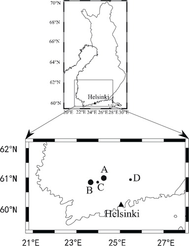
Lake Vanajavesi (61.13°N, 24.27°E) is located in southwestern Finland (Fig. 1). It is a large, shallow and eutrophic lake. The area is 113 km², and the mean and maximum depths are 7 and 24 m, respectively. The lake has a long eutrophication history with very poor water quality in the 1960s and 1970s. The ice season lasts 4–6 months, on average from December to April, and the thickness of ice reaches its annual maximum value of 45–60 cm in March. The ice and snow thickness may show distinct spatial variations due to snowdrift and heat flux from the lake water.

Fig. 1.  Geographical location of Lake Vanajavesi (A); surrounding observation sites Jokioinen meteorological observatory (B), Lake Kuivajärvi (C) and Lake Pääjärvi (D).

In the winter of 2008–2009, a field programme was performed in Lake Vanajavesi. Hydrographical surveys were made regularly, an automatic ice station was set up and optical investigations were performed (Jaatinen et al., 2010; Lei et al., 2011). The average maximum snow and ice thicknesses reached 15 and 41 cm, respectively, in March. The freezing and breakup dates were 1 January and 27 April, respectively.

Synoptic-scale weather conditions and regional climate over this area are represented by Jokioinen meteorological observatory (60.8°N, 23.5°E; WMO station 02863), located some 50 km southwest of Lake Vanajavesi (Fig. 1). The weather forcing data for the lake ice model consist of wind speed (V _a ), air temperature (T _a ), relative humidity (Rh), cloudiness (CN) and precipitation (Prec), collected at 3-hour time intervals. For the present modelling work, we interpolated data to 1-hour intervals. The snow thickness on land is also available from Jokioinen.

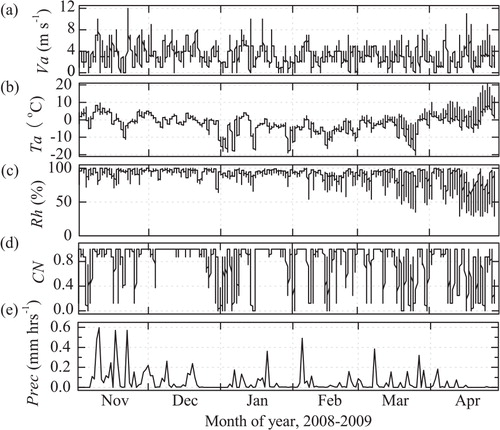
The winter 2008–2009 was mild (Fig. 2). The early winter was warm, with average air temperature of 0.6°C in November and December preventing Lake Vanajavesi from freezing. From late December to the end of March, the air temperature was permanently below the freezing point, on several occasions approaching −20°C and thereafter increased gradually to above 0°C. The ice season 2008–2009 can be divided into two phases: ice growth (January–March) and melting (April). The corresponding average air temperatures were −4.4 and +4.3°C, respectively. The total precipitation from November to April was 234 mm. During the ice growth season, however, the snow accumulation was merely 92 mm water equivalent (WEQ).

Fig. 2.  Time series of wind speed (a), air temperature (b), relative humidity (c), cloudiness (d) and precipitation (e). The data were initially observed at 3-hour time interval.

2.2. Climatological for long-term simulations

Monthly mean meteorological observations from the Jokioinen observatory in the climatological normal period 1971–2000 (http://en.ilmatieteenlaitos.fi/normal-period-1971–2000) were used for the forcing to investigate ice climatology (Table 1, based on Drebs et al., 2002). The mean air temperature was −2.8°C in November–April, 1.3°C less than in the winter 2008–2009. The precipitation was 232 mm, about the same that was observed in 2008–2009, but during the ice growth season, the average snow accumulation was 145 mm WEQ or 58% more than in 2008–2009.

Table 1. The monthly mean meteorological data for 1971–2000 (Drebs et al., 2002; h′ _s is snow thickness on the 15th of each month; Ph _s is the portion of precipitation contributing to the snow accumulation)

Month	V a (m s^−1)	T a (°C)	CN	Rh (%)	Precipitation (mm month^−1)	h′ s (cm)	Ph s (%)
October	3.8	4.6	0.76	88	59	0	–
November	3.9	−0.4	0.83	90	57	2	X
December	3.9	−4.1	0.81	90	45	9	46
January	3.8	−5.9	0.79	89	41	19	77
February	3.7	−6.5	0.74	87	29	29	94
March	3.8	−2.7	0.68	82	30	31	23
April	3.7	2.7	0.7	74	32	10	X
May	3.7	9.5	0.62	64	35	X	X

The average freezing and ice breakup dates of Lake Vanajavesi were 30 November and 30 April, respectively, in 1971–2000 (Korhonen, 2005). A large variation occurred in these dates in individual years. The earliest freezing date was 28 October and the latest one was 28 January. For the ice breakup, the earliest and latest dates were recorded as 1 April and 27 May, respectively.

Due to the lack of snow and ice thickness data in Lake Vanajavesi, the observations of Lake Kuivajärvi (Korhonen, 2005), located about 60 km southwest of Lake Vanajavesi, were used as the validation data. It can be assumed that the climatological conditions are the same in these two lakes.

3. The lake ice thermodynamic model

3.1. Surface temperature and surface heat/mass balance

The thermodynamic lake ice model HIGHTSI solves the surface temperature (T _sfc) from a detailed surface heat balance equation using an iterative method:1

where α is the albedo, Q _s is the incoming solar radiation at the surface, I ₀ is the portion of solar radiation penetrating below the surface layer and contributing to internal heating of the snow and ice, Q _d and Q _b are the incoming and outgoing longwave radiation, respectively, Q _h is the sensible heat flux, Q _le is the latent heat flux, F _c is the conductive heat flux coming from below the surface and F _m stands for melting. All fluxes are positive towards the surface.

In HIGHTSI, I ₀ is explicitly parameterised based on the fact that penetrating solar radiation is strongly attenuated along the vertical depth immediately below the surface (Grenfell and Maykut, 1977). The term (1−α)Q _s−I ₀ thus represents the part of short-wave radiation contributing to the surface heat balance. It depends on the surface layer (i.e. the first layer of snow or ice in model) thickness (Launiainen and Cheng, 1998; Cheng, 2002; Cheng et al., 2008). Equation (1) serves as the upper boundary condition of the HIGHTSI model. If the surface temperature is at the melting point (T _f), excessive heat (F _m) is used for melting: dh/dt=−F _m/ρL _f, where h is the thickness of snow or ice, ρ is the density of snow or ice and L _f is the latent heat of fusion.

The albedo is critical for snow and ice heat balance. A parameterisation suitable for the Baltic Sea coastal snow and land-fast ice is selected in this study (Pirazzini et al., 2006):2

where α _s and α _i are snow and ice albedo, α _s=0.75, and h _s and h _i are the snow and ice thickness, respectively.

Incoming solar or longwave radiation can be either parameterised for estimation from cloudiness, temperature and humidity or directly obtained from an NWP model. For the solar radiation, we applied the clear sky equation of Shine (1984) with cloud effect of Bennett (1982):3

where S is the solar constant, Z is the solar zenith angle, e is the water vapour pressure (mbar) and CN is the cloudiness ranging between 0 and 1. The net longwave radiative flux (Q _d−Q _b) was calculated by:4

where the first term on the right-hand side represents the incoming longwave radiation (Efimova, 1961, with cloud effect of Jacobs, 1978), the second term is outgoing longwave radiation, σ _s is the Stefan–Boltzmann constant and ɛ is the surface emissivity, which ranges from 0.96 to 0.99 (Vihma, 1995).

The surface turbulent heat fluxes were parameterised on the basis of atmospheric stratification. The sensible heat Q _h and latent heat Q _le were calculated by:5 6

where T _a−T _sfc is the difference between air and surface temperature, q _a−q _sfc is the difference between air and surface specific humidities, V _a is the wind speed, R _l the enthalpy of sublimation of water, ρ _a is the density of air, c _a is the specific heat of air and C _H and C _E are the bulk transfer coefficients estimated using the Monin–Obukhov similarity theory (Launiainen and Cheng, 1995).

The surface conductive heat flux was determined by:7

where T is temperature, z is the depth below the surface and k is the thermal conductivity in the surface layer.

3.2. Snow and ice evolution

Snow cover evolution was modelled taking into account several factors: precipitation, packing of snow and melt–freeze metamorphosis. Packing depends on precipitation, air temperature and wind speed, which are obtained from observations or from an NWP model. A temperature criterion was set (T _a<0.5°C) to decide whether precipitation is solid or liquid. The impact of wind on snow accumulation is regarded as a model uncertainty. In the climatological sense, however, one may have a rough idea of the influence of wind on snow accumulation by comparing the measured precipitation and snow thickness (cf. Section 4.2). In addition to the surface melting, snow and ice temperature may reach the melting point below the surface because of the absorption of the penetrating solar radiation. The subsurface melting is then calculated according to Cheng et al. (2003).

In boreal lakes, snow may contribute significantly to the total ice thickness. Snow-load can cause a negative ice freeboard and consequent formation of a slush layer by mixing of lake water and snow. A slush layer can also be formed by percolation of snow meltwater or liquid precipitation. Freezing of slush into ice was calculated by the heat flux divergence:8

where h _si is snow–ice thickness and ρ _si is the density of snow–ice. Slush formation from flooding was calculated according to Leppäranta (1983). After its formation, snow–ice becomes an internal layer part of the ice sheet.

The density of snow is a prognostic variable, calculated according to Anderson (1976):9

where c ₁ and c ₂ are empirical constants and w _s is the mass of snow in the above layer in WEQ. In this study, we set c ₁=5 m⁻¹ h⁻¹ and c ₂=21 m³ kg⁻¹.

The snow and ice temperatures were solved from the heat conduction equation:10

where q(z, t) presents the solar radiation penetrating into the snow and ice based on an exponential attenuation law: q _s(z, t)=(1−α _s,i)I ₀ exp(−κ _s,i z), where κ _s,i is the extinction coefficient of snow or ice.

The integral interpolation method was applied to build up the numerical scheme (Cheng, 2002). A high spatial resolution (e.g. 10 layers in the snow and 20 layers in the ice) ensures that the response of the snow and ice temperature regime to the absorption of solar radiation near the surface is correctly resolved. In the case of snow on top of the ice, the snow–ice interface temperature is calculated via a flux continuity equation:11

Heat and mass balances at the ice bottom served as the lower boundary condition:12

where F _w is the heat flux from water to ice. The model parameters for this study are summarised in Table 2.

Table 2. Model parameters found in the literature

Parameter	Value	Source
Extinction coefficient of lake ice (κ i)	1.5–17 m^−1	Heron et al. ( 1994); Arst et al. (2006); Lei et al. (2011)
Extinction coefficient of snow (κ s )	6–20 m^−1	Patterson et al. ( 1988); Arst et al. (2006); Lei et al. (2011)
Lake ice density (ρ i)	910 kg m^−3	Corresponds to 1% gas content
Initial snow density (ρ s)	330 kg m^−3	Leppäranta and Kosloff ( 2000)
Surface emissivity (ɛ)	0.97	Vihma (1995)

The freezing date in HIGHTSI is provided as the initial condition by a thin ice layer (0.02 m). If the weather conditions do not favour ice growth, HIGHTSI will resume the initial ice thickness. The first day when ice starts to grow successively is defined as the freezing date. It is clear that this is a crude approximation to obtain the freezing date, but once the ice growth has started, the model catches up well with the nature.

4. Results and discussion

4.1. Seasonal study for the winter 2008–2009

The ice season 2008–2009 lasted 4 months. Model simulations were started up in the beginning of January from the initial snow and ice thicknesses of 0.5 and 2 cm, respectively. The simulated snow thickness agreed well with the observations (Fig. 3), showing that the model can well reproduce the total snow accumulation and the snowmelt. Snow thickness over land, measured in Jokioinen, is also shown in Fig. 3. A previous study by Kärkäs (2000) has indicated that the snow cover on land is on average 2.3 times thicker than on lake ice in this region, based on monthly snow measurements from January to April during a 10-year period (1971–1980) in Lake Pääjärvi (61.07°N, 25.14°E). In the present case, the ratio between the observed mean snow depth in Jokioinen and the modelled average snow depth over the Lake Vanajavesi ice was 2.1.

Fig. 3.  Time series of observed and modelled snow and ice thickness. The dark grey line and the asterisk are the observed snow thickness in Jokioinen and on Lake Vanajavesi, respectively. The black dashed and solid lines are modelled snow and ice thickness (reference experiment), respectively. The circles are the observed average ice thickness, and the spatial standard deviation is indicated by the vertical bar.

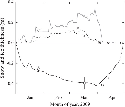
The modelled ice thickness fitted well with the field measurements, and particularly the ice breakup date was close to the observation. In the beginning of January, the ice grew rapidly in response to the very cold air temperature. As soon as the snow depth had reached about 10 cm, the speed of ice growth reduced significantly because of the insulating effect of snow. Snow to snow–ice transformation also contributed a little to the total ice thickness in the late season. A 9-cm slush layer and a 1-cm snow–ice layer were measured on 18 March (Lei et al., 2011), while the model prediction was a 5-cm slush layer and no snow–ice. This error is likely due to overestimation of snow density in the model. Later, on 7 April, a 2-cm slush layer and a 5-cm frozen slush layer were observed (Lei et al., 2011), while in our simulation these values had become 2.9 and 2.7 cm, respectively, by the end of March. On 14 April, a 3-cm slush layer was still observed but snow–ice had disappeared. The melt rate of ice was 1 cm d⁻¹ from 7 April to 14 April (Lei et al., 2011), both in the model and in the observations. The melting of ice started in the beginning of April, as soon as snow had gone, and it accelerated towards the breakup (Fig. 3). The melting period lasted 30 d, with mean melt rate of 1.3 cm d⁻¹.

The heat flux from lake water to the ice bottom has been earlier examined in the nearby Lake Pääjärvi by Shirasawa et al. (2006) and Jakkila et al. (2009). The magnitude was found to be 3–10 W m⁻² based on field data. In freshwater lakes, before freezing the water column is well mixed down to 1–4°C depending on the autumn wind conditions, lake size and land area around. Thereafter, inverse winter stratification is set up, and once ice is formed, further mixing is strongly limited. The water temperature structure under the ice is usually quite stable with a very small heat flux out from the water body.

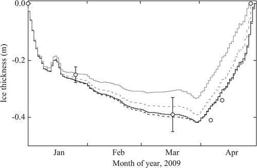
To examine the sensitivity of ice thickness to the heat flux from the water, model runs were carried out with different fixed heat flux levels: 0, 0.5, 2 and 5 W m⁻² (Fig. 4). In the early winter, there was a very large temperature gradient across the ice sheet, and the heat conduction through the ice and the consequent ice growth rate were large. As soon as the ice thickness has reached about 20 cm and there is also snow on the ice, the heat conduction is reduced and closer to the heat flux from the water. Ice may then even melt from the bottom. The examined variations of the heat flux from water can alter the maximum ice thickness by ±3.4 cm, as compared to the results from the optimised reference simulation, where the heat flux from water to ice was 0.5 W m⁻². This level was quite low, of the same magnitude than the molecular conduction of heat. It is much less than what has been earlier obtained in Lake Pääjärvi, which is deeper and also has more groundwater inflow in the mass balance. A large heat flux from the water would give less ice thickness and earlier breakup date. For example, a 1 W m⁻² heat flux melts about 1 cm ice in a month, and for the mean melt rate of 1.3 cm d⁻¹ ice breakup would be about 1 d earlier.

Fig. 4.  Time series of observed and simulated ice thickness based on varying heat flux from water: 0 W m⁻² (black dashed), 0.5 W m⁻² (black solid; reference experiment), 2 W m⁻² (grey dashed) and 5 W m⁻² (grey solid). Measurements of ice thickness are shown as in Fig. 3.

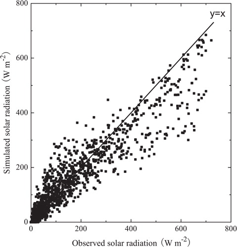
The parameterised solar radiation may be an underestimate. The uncertainties are due to the effect of clouds as well as due to multiple scattering in the air (Shine, 1984; Wendler and Eaton, 1990). Fig. 5 gives the observations and calculations for Jokioinen in January–April 2009. The largest differences, 200 W m⁻², appeared mostly in March–April. Then, on average, underestimation of solar radiation may account for 7 W m⁻² of the total net radiative flux. This amount of energy can offset 3 cm of the ice thickness and lead to a 5-d shift in the ice breakup date.

Fig. 5.  Calculated and observed incoming short-wave radiative flux under clear and cloudy sky conditions. The data cover the winter 2008–2009 from January to April. Goodness of fit for the whole ice season's data was R ²=0.92 (n=2880).

The surface temperature reflects the ice thickness during the cold season, because the ice thickness impacts the strength of the insulation between the lake water body and the atmosphere. By applying the heat conduction law (Eq. 1), we can solve the ice thickness as a function of the surface temperature or vice versa. The inverse procedure is used in thermal remote sensing for mapping the sea ice thickness (Rothrock et al., 1999; Leppäranta and Lewis, 2007; Mäkynen et al., 2010; Wang et al., 2010). In weather forecasting, the surface temperature is needed as a boundary condition for the atmosphere. Due to ice–atmosphere coupling, NWP needs an ice model to obtain the surface temperature of lakes in winter.

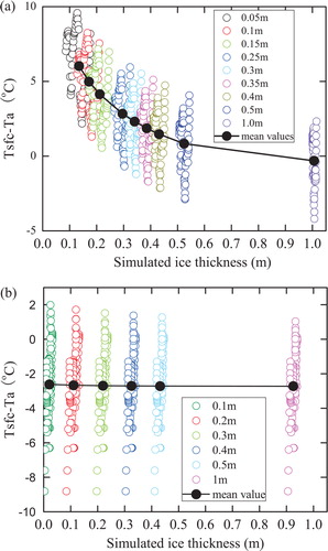
To examine the sensitivity of surface temperature on ice thickness, a number of seasonal model runs were performed with different initial ice thicknesses. The results are given in Fig. 6. In a cold period (Fig. 6a), thin ice grows faster than thick ice because of stronger heat conduction from warm water to the cold atmosphere, and as a consequence, its surface is warmer. If we look into the average situation, we can see that the surface temperature dependence on ice thickness is more pronounced for ice thickness <0.5 m, as noted by Leppäranta and Lewis (2007). But the daily cycle is seen in the surface temperature, and therefore inversion of surface temperature to ice thickness would need an ice model with full heat conduction equation. In a warm period (Fig. 6b), the ice warms up and the temperature approaches isothermal conditions at 0°C. Next, heat conduction through the ice stops, and the surface does not feel the thickness of ice any more. Then, nighttime cooling reduces the surface temperature down, but the time scale is too short for cooling to reach the lower boundary of the ice sheet to provide thickness information.

Fig. 6.  Surface temperature versus ice thickness: for a cold period 0000 hr 3 January through 2300 hr 5 January (a); for a warm period 0000 hr 8 April through 1300 hr 11 April (b). In both cases, the snow was set to be zero for simplicity.

4.2. Climatological simulation for the normal period 1971–2000

Ice climatology was examined using the mean monthly atmospheric conditions as the forcing data. The model runs were started up in the beginning of November. The initial snow and ice thicknesses were assumed to be 0.5 and 2 cm, respectively.

The first simulation suggested that snow thickness was likely overestimated by the model, particularly in early winter, if the monthly mean precipitation rate was directly used as the model input. This led to underestimation of ice thickness. In the ice growth season, one can estimate the ratio of snow accumulation from precipitation to the measured snow depth on ground by using climatological snow thickness and precipitation data (Table 1). In the early winter, the coherence was weak, probably because a part of the precipitation had fallen as liquid water. Additionally, snowdrift may transport snow away from the lake surface. The best coherence between precipitation and snow thickness was obtained in February, when 94% of the precipitation contributed to snow accumulation. In early spring, due to the melting effect, the discrepancy between precipitation and snow depth became again larger. We therefore took a simple calculation procedure to define a solid portion of the precipitation in each winter month (Table 1). The result was used as the input into the climatological simulations.

Figure 7 shows the result using the modified snow accumulation algorithm. The simulated freezing and ice breakup dates were 8 November and 12 May, and the duration of ice season was 184 d. Compared to observations (from 30 November to 30 April, altogether 152 d), the simulated ice season was considerably longer than the mean ice season in 1971–2000. The modelled freezing date turned out to be 22 d too early and the breakup date 12 d too late. In the simulations, the treatment of the freeze-up was biased, since in the model the cooling process of lake water was missing, which led to the too early freezing. Differences between the simulated and observed ice breakup dates may be due to two reasons. First, if the initialisation of melting season is delayed, this shifts the breakup date. Secondly, in the melting season, the ice strength decreases due to internal deterioration, and wind forcing is able to break the ice. Ice may then drift, which further induces turbulent mixing and heat transfer in the water body (Wake and Rumer, 1983; Burda, 1999; Leppäranta, 2009).

Fig. 7.  Time series of simulated snow (grey line) and ice (black line) thickness. The circles show the mean ice thickness observed in the middle of each month in Lake Kuivajärvi (60.76°N, 23.88°E; cf. Fig. 1) located southwest (60 km) from Lake Vanajavesi.

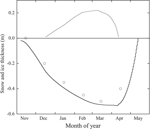
The dots in Fig. 7 depict the mean observed ice thickness in Lake Kuivajärvi during 1961–2000 (Korhonen, 2005). Compared with the model simulation, the HIGHTS bias was 5 cm, the correlation coefficient was 0.97 and the standard deviation was 3 cm. We can conclude that HIGHTSI can produce climatological ice thickness in reasonably good agreement with the regional measurements.

The role of the daily cycle in the monthly lake ice climatology was investigated with 10-d model runs for each month in November–April. The monthly air temperature statistics, snow and ice conditions and model results are given in Table 3. For each month, a sinusoidal daily air temperature cycle (model experiment I) was created by the mean value of the climatological normal period (model experiment II; cf. Table 1) ± the standard deviation of 2008–2009 (Table 3). For comparison, the model runs with monthly mean temperature were also given. The snow thickness remained as the climatological monthly mean for the sake of simplicity. The initial ice thickness (on the first day of each month) was taken as the monthly mean.

Table 3. Initial setup (T _a, h _s, h _i) for 10-d simulations and simulated ice growth rate (dh _i/dt)

	T a (°C)				dh i /dt (cm d^−1)
Month	I	II	Initial h s (m)	Initial h i (m)	I	II
November	[−4.2, 3.4]	−0.4	0	0.01	0.42	0.47
December	[−6.5, −1.7]	−4.1	0.03	0.10	0.60	0.58
January	[−11.7, 0.1]	−5.9	0.05	0.25	0.45	0.49
February	[−10, −3]	−6.5	0.10	0.35	0.37	0.37
March	[−7, 1.6]	−2.7	0.10	0.45	0.35	0.20
April	[−2.5, 7.8]	2.7	0	0.45	−0.59	−0.03

The time series of simulated ice thickness are shown in Fig. 8. In the model experiment I, the ice growth showed a maximum rate of 6 cm in 10 d in December. This rapid growth was because the snow is relatively thin. From January to March, the snow was thicker and the ice thickness could still increase by 4–5 cm in 10 d. This growth rate is commonly seen as the climatological ice growth rate in the winter season. In April, the decrease of ice thickness was evidently due to the combined effect of the warm air temperature and diurnal variation of the incoming solar radiation. The ice melt rate was ca. 0.6 cm d⁻¹.

Fig. 8.  Ten-day modelled ice thickness based on air temperature varying sinusoidally (red lines) and constant mean values (black lines) for each winter month: November (a); December (b); January (c); February (d); March (e) and April (f).

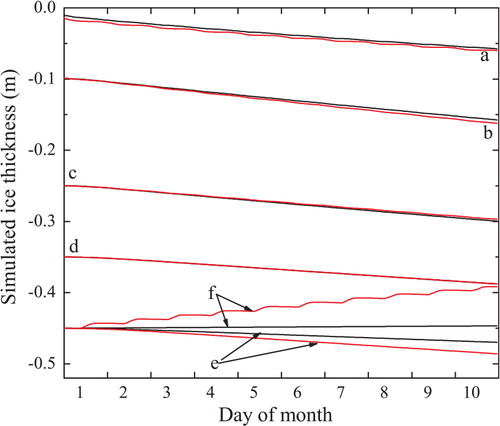
Model runs with constant air temperature resulted in quite similar ice growth compared to model runs with daily cycle in November–February (Fig. 8). This may be anticipated since the daily cycle is not strong in mid-winter in latitudes this high (61°N). In March, the mean temperature was −2.7°C with daily amplitude of 4.5°C, and more ice was produced when the daily cycle was included (Table 3). In April, the ice started to melt in both model runs. However, with the daily cycle much more ice could be melted. The freezing point temperature (0°C) can be seen as the threshold value to determine the impact of the daily cycle. In early spring, the nighttime temperature often drops below 0°C, helping to maintain the ice growth. However, if the diurnal temperature range is dominantly positive, the ice melting will accelerate.

Overall, lake-ice processes are closely associated with weather conditions from autumn through spring. The freezing of lake surface largely depends on the lake heat storage and the cooling rate of the air temperature during the autumn. Ice breakup can be explained mainly by the net solar radiation (e.g. Leppäranta, 2009). Figure 9 shows a comparison of the results of the HIGHTSI simulations using climatological forcing (Table 1), with the air temperature artificially shifted by ±1 or ±5°C. Compared to the reference run (Fig. 8), shifting by ±1°C may lead to about 5 d change of freezing date and 8 d change of breakup date. These values are close to 5 d for both dates, obtained by linear regression on lake phenology time series for lakes in southern Finland (Palecki and Barry, 1986). The breakup date seems to be more sensitive to the air temperature in the model.

Fig. 9.  Model sensitivity to the air temperature. The black solid line is the reference of present climate. The grey solid (dashed) line and light grey solid (dashed) line are modelled ice thickness based on air temperature decreasing (increasing) 5 and 1°C, respectively.

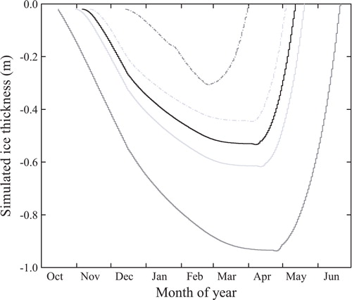
Changes in the freezing date depend on the local atmospheric autumn cooling rate and are therefore different in maritime and continental climate zones (Leppäranta, 2009). But the relation between the ice breakup date and spring warming rate is unclear. Nonaka et al. (2007) found that a 1°C increase in air temperature can lead to an earlier ice breakup by 3–10 d. Here, model runs suggested an overall ice season length to decrease by 13 d for 1°C change in climate. The change of seasonal average ice thickness was ±17% or ±6 cm from 36 cm for ±1°C air temperature change. If the air temperature shifted by +5°C, the ice season would start in the middle of December and end in early April. In contrast, if the air temperature shifted by −5°C, the ice season would start in early October and end in mid-June. In these cases, the maximum ice thickness would change by −22 and 41 cm. Changes with ±5°C were not symmetric, because the air temperature change also influenced the length of the ice season, and ice grew to a first order in proportion to the square root of the freezing-degree days.

4.3. Surface heat balance

The surface heat fluxes reflect the ice growth and melt. Components of the surface energy balance (Eq. 1) were calculated for the winter 2008–2009 and for the climatological normal period 1971–2000 (Table 4). The results are in agreement with Jakkila et al. (2009) for Lake Pääjärvi, located in a nearby region.

Table 4. The daily mean heat fluxes contributing to the surface heat balance (W m⁻²). The columns are surface layer absorption of solar radiation, net longwave radiation, sensible heat flux, latent heat flux, conductive heat flux from below and heat flux for melting

	Month	(1−α s,i )Q s − I 0	Q b −Q d	Q h	Q le	F c + F m
2008–2009	December	0.94	−18.38	6.37	0.55	10.52
	January	0.55	−24.05	−5.71	−6.77	35.98
	February	2.30	−17.99	0.84	−4.55	19.41
	March	5.73	−16.91	3.94	−6.71	13.95
	April	21.36	−7.26	21.84	−8.48	−27.46
1971–2000	December	0.17	−21.58	−5.53	−10.84	37.78
	January	0.60	−22.25	2.07	−4.83	24.41
	February	2.17	−33.93	7.78	−2.27	26.25
	March	4.45	−25.26	5.43	−8.91	24.29
	April	19.27	−8.93	18.68	−4.65	−24.37

In both cases, the lake surface lost heat from December to March and gained heat in April. In December 2008, heat loss from the surface was less intensive compared with January 2009. This may partly explain the delayed freezing date. In contrast, we can see that a strong heat loss occurred in December for the climatological normal period 1971–2000. This agrees with the fact that the freezing date is normally in December. A strong heat loss in January 2009 occurred during the cold period (Fig. 2b).

Analysing the net surface heat flux for February and March, it is seen that in 2009 the negative surface heat balance was weaker than in 1971–2000. In April 2009 a larger positive surface heat balance could have led to an earlier breakup date than during 1971–2000. It is clear that the weather conditions in early winter and in early spring are critical for the determination of the length of the lake ice season. The net longwave radiation dominates the surface heat balance in the winter season, while the net solar radiation is critical for melting.

5. Conclusions

The ice cover in Lake Vanajavesi has been investigated with a one-dimensional thermodynamic model HIGHTSI. A case study was performed for one ice season, and a 30-year period (1971–2000) was examined for ice climatology. The results were good as compared with the validation data. The model was then applied to examine the response of the lake ice season to climate change. The novel features of the HIGHSTI for lake investigations are the advanced treatments of superimposed ice, stability-dependent turbulent heat fluxes and coupling of snow and ice layers.

The modelled snow thickness was produced from measured precipitation and a simple model for snow metamorphosis. This made snow a free model variable. Snow accumulates during cold periods, while it may decrease due to transformation into snow–ice or melting. In the case study ice season, snow thickness and snow–ice formation were reproduced well. But due to lack of long-term data on ice stratigraphy, the modelled snow–ice cannot be validated quantitatively for the climatological simulation. Our calculations suggested that on an average 16% of the snowfall contributed to the total ice thickness (53 cm) with a 10-cm snow–ice layer.

The model experiments produced an estimate for the heat flux from water to ice by tuning. The result was a small value, 0.5 W m⁻², corresponding to the magnitude of molecular heat conduction. The annual maximum ice thickness could change up to 10 cm in response to a change of the level of the heat flux to 5 W m⁻². The ice breakup date would be affected by 5 d. The air temperature is the prevailing factor that affects the lake ice season. The diurnal variation of air temperature has no significant influence on ice thickness in the growth season but gives large impact on the ice thickness in late winter and in the melting season.

The surface temperature and the thickness of ice are closely related. The model simulations showed that inversion of the surface temperature for ice thickness by thermal remote sensing is feasible for thin ice (< 0.5 m), but then the timing of measurement is critical and the full heat conduction equation needs to be used. The model simulations showed that in NWP and climate modelling, inclusion of a proper lake ice model would produce a better surface temperature and consequently improve the quality of the predictions.

Climate change may have a dramatic influence on the course of the ice season. The annual maximum ice thickness was 53 cm in Lake Vanajavesi in 1971–2000, about 11 cm more than in winter 2008–2009. The corresponding mean air temperature for 1971–2000 was about 1.5°C lower than the temperature in winter 2008–2009. Our model experiments, based on changing the air temperature level in the climatological simulations, showed that the air temperature shifts affect the freezing date by 5 d °C⁻¹ and the breakup date by 8 d °C⁻¹.

Future studies are needed to couple the present model with a lake water body model to predict better the autumn cooling of the water and the consequent freezing date. The timing of the onset of snow and ice melting in the model is the most critical point for further improvements.

6. Acknowledgements

This research was supported by YMPANA (Development of automatic monitoring system for Lake Vanajavesi) project, National Natural Science Foundation of China (Grant No. 51079021, 40930848 and 50879008) and the Norwegian Research Council (Grant No. 193592/S30). The CIMO scholarship from Finnish Ministry of Education is acknowledged for funding the first author to work in Finland. Comments from the anonymous reviewers were very helpful to improve this paper. We are very grateful to Dr. Laura Rontu and Dr. Timo Vihma for providing various inspiring comments and suggestions during the preparation of this manuscript.

References

- Anderson, E. 1976. A point energy and mass balance model for a snow cover. NOAA Technical Report. NWS 19, 150 pp.
- Arst H. Erm A. Leppäranta M. Reinart A. Radiative characteristics of ice-covered freshwater and brackish water bodies. Proc. Estonian Acad. Sci. Geol. 2006; 55: 3–23.
- Bennett T. J. A coupled atmosphere-sea-ice model study of the role of sea ice in climatic predictability. J. Atmos. Sci. 1982; 39: 1456–1465.
- Brown L. C. Duguay C. R. The response and role of ice cover in lake-climate interactions. Prog. Phys. Geogr. 2010; 34: 671–704.
- Burda N. Y. Computer simulation for Ladoga Lake ice dynamics based on remotely sensed data. Int. Geosci. Remote Sensing Symp. 1999; 2: 937–939.
- Cheng, B. 2002. On modeling of sea ice thermodynamics and air-ice coupling in the Bohai Sea and the Baltic Sea. Finnish Institute of Marine Research – Contributions. 5, 38 pp. ( Ph.D thesis)
- Cheng B. Vihma T. Launiainen J. Modelling of the superimposed ice formation and sub-surface melting in the Baltic Sea. Geophysica. 2003; 39: 31–50.
- Cheng, B, Zhang, Z, Vihma, T, Johansson, M, Bian, L and co-authors. 2008. Model experiments on snow and ice thermodynamics in the Arctic Ocean with CHINAREN 2003 data. J. Geophys. Res. 113, C09020., 10.3402/tellusa.v64i0.17202.
- Drebs A. Nordlund A. Karlsson P. Helminen J. Rissanen P. Climatological Statistics of Finland 1971–2000. Finnish Meteorological Institute: Helsinki, 2002
- Duguay, C. R, Flato, G. M, Jeffries, M. O, Ménard, P, Morris, K and co-authors. 2003. Ice-cover variability on shallow lakes at high latitudes: model simulations and observations. Hydrol. Proces. 17, 3464–3483.
- Eerola K. Rontu L. Kourzeneva E. Shcherbak E. A study on effects of lake temperature and ice cover in HIRLAM. Boreal Env. Res. 2010; 15: 130–142.
- Efimova N. A. On methods of calculating monthly values of net longwave radiation. Meteor. Gidrol. 1961; 10: 28–33.
- Ellis A. W. Johnson J. J. Hydroclimatic analysis of snowfall trends associated with the North American Great Lakes. J. Hydrol. 2004; 5: 471–486.
- Flato G. M. Brown R. D. Variablility and climate sensitivity of landfast Arctic sea ice. J. Geophys. Res. 1996; 101: 25767–25777.
- Grenfell T. C. Maykut G. A. The optical properties of ice and snow in the Arctic Basin. J. Glaciol. 1977; 18: 445–463.
- Heron R. Woo M. K. Decay of a High Arctic lake-ice cover: observations and modelling. J. Glaciol. 1994; 40: 283–292.
- Jaatinen, E, Leppäranta, M, Erm, A, Lei, R, Pärn, O and co-authors. 2010. Light conditions and ice cover structure in Lake Vanajavesi. In: Proceedings of the 20th IAHR Ice Symposium, Paper #79. Department of Physics, University of Helsinki, Finland.
- Jacobs, J. D. 1978. Radiation climate of Broughton Island. In: Energy Budget Studies in Relation to Fast-ice Breakup Processes in Davis Strait, Occasional Paper. R. G. Barry and J. D. Jacobs). Institute of Arctic and Alpine Research, University of Colorado, Boulder, 26, pp. 105–120.
- Jakkila J. Leppäranta M. Kawamura T. Shirasawa K. Salonen K. Radiation transfer and heat budget during the melting season in Lake Pääjärvi. Aquat. Ecol. 2009; 43: 681–692.
- Kärkäs E. The ice season of Lake Pääjärvi in southern Finland. Geophysica. 2000; 36: 85–94.
- Korhonen, J. 2005Suomen vesistöjen jääolot [Ice Conditions in Lakes and Reviers in Finland]. Suomen ympäristö 751. Finnish Environment Institute. (in Finnish with English summary).
- Launiainen, J and Cheng, B. 1995. A simple non-iterative algorithm for calculating turbulent bulk fluxes in diabatic conditions over water, snow/ice and ground surface. Report Series in Geophysics. Department of Geophysics, University of Helsinki, 33 pp.
- Launiainen J. Cheng B. Modelling of ice thermodynamics in nature water bodies. Cold Reg. Sci. Technol. 1998; 27: 153–178.
- Lei R. Leppäranta M. Erm A. Jaatinen E. Pärn O. Field investigations of apparent optical properties of ice cover in Finnish and Estonian lakes in winter 2009. Est. J. Earth Sci. 2011; 60: 50–64.
- Leppäranta M. A growth model for black ice, snow ice and snow thickness in subarctic basins. Nordic Hydrol. 1983; 14: 59–70.
- Leppäranta M. A review of analytical models of sea-ice growth. Atmos. Ocean. 1993; 31: 123–138.
- Leppäranta, M. 2009. Modelling the formation and decay of lake ice. In: Climate change impact on European lakes. G. George. Springer, Berlin. Aquatic Ecology Series. 4, pp. 63–83.
- Leppäranta M. Kosloff P. The thickness and structure of Lake Pääjärvi ice. Geophysica. 2000; 36: 233–248.
- Leppäranta M. Lewis J. E. Observations of ice surface temperature and thickness in the Baltic Sea. Int. J. Remote Sens. 2007; 28: 3963–3977.
- Leppäranta, M and Uusikivi, J. 2002. The annual cycle of the Lake Pääjärvi ice. Lammi Notes 29. Lammi Biological Station, University of Helsinki.
- Liston G. E. Hall D. K. An energy-balance model of lake-ice evolution. J. Glaciol. 1995; 10: 373–382.
- Livingstone D. M. Lake oxygenation: application of a one-box model with ice cover. Int. Rev. Ges. Hydrol. 1993; 78: 465–480.
- Maykut G. A. Untersteiner N. Some results from a time-dependent thermodynamic model of sea ice. J. Geophys. Res. 1971; 76: 1550–1575.
- Mäkynen, M, Similä, M, Cheng, B, Laine, V and Karvonen, J. 2010. Sea ice thickness retrieval in the Baltic Sea using MODIS and SAR data. In: Proceeding of SeaSAR2010, Frascati, Italy, ESA SP-679.
- Mironov, D, Heise, E, Kourzeneva, E, Ritter, B, Schneider, N and co-authors. 2010. Implementation of the lake parameterisation scheme Flake into the numerical weather prediction model COSMO. Boreal Env. Res. 15, 218–230.
- Nonaka T. Matsunaga T. Hoyano A. Estimating ice breakup dates on Eurasian lakes using water temperature trends and threshold surface temperatures derived from MODIS data. Int. J. Remote Sens. 2007; 28: 2163–2179.
- Palecki M. A. Barry R. G. Freeze-up and break-up of lakes as an index of temperature changes during the transition seasons: a case study for Finland. J. Appl. Meteorol. Climatol. 1986; 25: 893–902.
- Patterson J. C. Hamblin P. F. Thermal simulation of a lake with winter ice cover. Limnol. Oceanogr. 1988; 33: 323–338.
- Pirazzini R. Vihma T. Granskog M. A. Cheng B. Surface albedo measurements over sea ice in the Baltic Sea during the spring snowmelt period. Ann. Glaciol. 2006; 44: 7–14.
- Rothrock D. A. Yu Y. Maykut G. A. Thinning of the Arctic sea-ice cover. Geophys. Res. Lett. 1999; 26: 3469–3472.
- Rouse, W. R, Blanken, P. D, Duguay, C. R, Oswald, C. J and Schertzer, W. M. 2008b. Climate–lake interations. In: Cold Region Atmospheric and Hydrologic Studies: The Mackenzie GEWEX Experience. (ed. MK. Woo). Vol. 2, Springer, Berlin, pp. 139–160.
- Rouse, W. R, Binyamin, J, Blanken, P. D, Bussières, N, Duguay C. R and co-authors. 2008a. The influence of lakes on the regional energy and water balance of the central Mackenzie. In: Cold Region Atmospheric and Hydrologic Studies: The Mackenzie GEWEX Experience. (ed. MK. Woo). Vol. 1, Springer, Berlin, pp. 309–325.
- Salgado R. LE Moigne P. Coupling of the Flake model to the Surfex externalized surface model. Boreal Env. Res. 2010; 15: 231–244.
- Saloranta T. Modeling the evolution of snow, snow ice and ice in the Baltic Sea. Tellus. 2000; 52A: 93–108.
- Shine K. P. Parameterization of shortwave flux over high albedo surfaces as a function of cloud thickness and surface albedo. Quart. J. Roy. Meteor. Soc. 1984; 110: 747–764.
- Shirasawa, K, Leppäranta, M, Kawamura, T, Ishikawa, M and Takatsuka, T. 2006. Measurements and modelling of the water – ice heat flux in natural waters. In: Proceedings of the 18th IAHR International Symposium on Ice, Hokkaido University, Sapporo, Japan, pp. 85–91.
- Shirasawa, K, Leppäranta, M, Saloranta, T, Kawamura, T, Polomoshnov, A and co-authors. 2005. The thickness of coastal fast ice in the Sea of Okhotsk. Cold Reg. Sci. Technol. 42, 25–40.
- Vihma T. Subgrid parameterization of surface heat and momentum fluxes over polar oceans. J. Geophys. Res. 1995; 100: 22625–22646.
- Wake A. Rumer R. R. Great lakes ice dynamics simulation. J. Waterway Port Coast. Ocean Eng. 1983; 109: 86–102.
- Wang, X, Key, J. R and Liu, Y. 2010. A thermodynamic model for estimating sea and lake ice thickness with optical satellite data. J. Geophys. Res. 115, C12035., 10.3402/tellusa.v64i0.17202.
- Wendler, G and Eaton, F. 1990. Surface radiation budget at Barrow, Alaska. Theor. Appl. Climatol. 41, 107–115.
- Williams G. Layman K. L. Stefan H. G. Dependence of lake ice covers on climatic, geographic and bathymetric variables. Cold Reg. Sci. Technol. 2004; 40: 145–164.