Climate data for parameterisation of lakes in Numerical Weather Prediction models

ABSTRACT

In Numerical Weather Prediction (NWP), to initialise lake variables for parameterisation of lakes, lake climatology is required. We obtained model lake climatology through offline runs of a lake model FLake (Freshwater Lake model) with different values of lake depth parameter. As a result, a global dataset with the resolution of 1° was developed. To project lake climatology onto a particular NWP model grid, data are extracted from the dataset depending on the lake depth value provided on the target grid. To prevent drifting of the bottom temperature in warm deep lakes, relaxation to the long-term mean air temperature was applied in FLake. Lake model climatology was validated against observations for different types of lakes. We suppose that detected errors for boreal lakes in spring are connected with inaccuracies in forcing data, but further study of errors is needed.

• parameterisation of lakes
• surface processes
• lake climatology

1. Introduction

Atmospheric boundary layer structure and behaviour are strongly dependent on surface processes. There is a large contrast in surface properties and hence in fluxes of heat, moisture and momentum between inland water and land. At high latitudes, where lakes are seasonally covered by ice, processes in the surface layer over ice-covered and ice-free lakes are different. This makes the situation more complicated. With increasing of Numerical Weather Prediction (NWP) models' horizontal resolution, more and more territories covered by inland water bodies appear to be visible on the grid. Even very small lakes are visible on the NWP model grid when the mosaic tiling philosophy is applied, i.e. when every grid box is considered to be fractionally covered by different surface types and fractions are calculated from very high-resolution data. Thus, lakes should be represented in NWP models. In principle, we may represent lakes in a NWP model in different ways. A very simple way is to use lake climatology. Another way is to use lake observations processing them by the analysis system spreading information horizontally. Also we may parameterise lakes with a lake model. And the most complicated and the most accurate way is to assimilate lake observations into the lake model coupled with a NWP model. But in all cases, we need lake climatology. For the first two cases we need only lake surface climatology, for direct representation of lakes or for the background information of the analysis system. Lake surface climatology comprises the ice cover and the surface water/ice/snow temperatures. For the two other cases, to initialise the lake model variables in the very first forecast cycle of the NWP system, we also need climatological temperature profiles in lakes. At present, lakes are poorly represented in the operational NWP systems. One reason is the absence of suitable lake climate data. Instead of them, very approximate estimations or even surrogates are used in operational practice.

In principle, we may obtain lake climatology either from measurements or from model simulations. For lakes, there are measurements of different kinds, space-born and in situ. Space-born data cover large territories and have good spatial and temporal resolution. But they contain information only about the lake surface temperature and the ice coverage. This is sufficient only if we are going to apply simple approaches with climatology or with the analysis system to spread information horizontally. If we intend to apply a lake parameterisation, we need also temperature profiles in lakes, which are not available from the satellite observations. Time series of satellite observations are still too short to derive climate values. Very often space born measurements contain significant errors because of cloud contamination, fractional ice cover or inaccurate lake mask. In situ measurements are much more reliable. They may contain information not only about the lake surface temperature and ice coverage, but also about the vertical temperature profiles and ice thickness. However, in situ measurements are available only for some lakes. Besides, these data cannot be simply interpolated, as lake state depends not only on geographical coordinates and elevation, but also on the lake depth and on the water turbidity. Hence, it is easier to obtain lake climatology from simulations, and measurements may be used for validation.

If we are going to apply a lake parameterisation, we need climatological temperature profiles. In practice, there are two types of lake models applicable to parameterise lakes in operational NWP systems, one-dimensional and bulk models (e.g. Hostetler et al., 1993; Blenckner et al., 2002; Mironov, 2008). Both types need initialization of the ice depth and temperature profiles, although in a bulk model the latter may be represented parametrically. It is difficult to provide the climatological profiles, as they depend not only on season and coordinates, but also on lake parameters, such as lake depth and turbidity.

The first important requirement from NWP to any climatological dataset is global representation (as regional models do have an ambition to be easily applied to any region on the globe). The second requirement is the gridded form of information. Grids of NWP models differ. Normally, in NWP models, lakes are mapped from land cover datasets having a resolution of approximately 1 km. The resolution of a NWP model grid is usually coarser, so the fraction of lakes is calculated from these very fine-scale data. Then NWP models apply either the lake mask derived from the lake fraction, or the mosaic tiling philosophy, keeping every grid box being fractionally covered by lakes. In the first case, we treat all lakes in the atmospheric model domain, which are larger than the NWP grid mesh. In the second case, we consider even sub-grid lakes. In both cases, lake information is grid-dependent. Moreover, the field of lake coverage is basically discontinuous, with every lake having different depth, turbidity and other properties. Thus, information about the thermal state of lakes cannot be simply interpolated from one grid to another. Aggregation is only possible. Hence, in the most “expensive” case of tiling philosophy, we need global information about lake climatology on the very fine 1 km grid. To represent each individual lake of this size is a too ambitious task. Sometimes we do not even know if the individual lake is represented on our map or not, land cover datasets are not precise enough (Kourzeneva, 2010; Kourzeneva et al., 2012). However, we may be satisfied even with quite approximate information, as variables will be in future corrected either by a lake model or by observations.

In this paper we present a new model lake climate dataset for use in NWP. The dataset was obtained from the Freshwater Lake model (FLake; Mironov, 2008), 20-year offline runs differing in terms of the lake depth. We used atmospheric forcing data described in Sheffield et al. (2006). We explain also how to project the lake climate data onto the particular grid of a NWP model. Any type of grid and resolution are possible. The first version of the system was presented in Kourzeneva (2010). The most important innovation in the new version presented here is the using of the full 20-year lake model run instead of a pseudo-periodic solution. We executed the full run because the pseudo-periodic solution is not necessarily attainable. We used the new atmospheric forcing data set with finer resolution than earlier. Further, we implemented a relaxation of the bottom temperature fixing the problem of warm deep lakes. Finally, we verified our dataset against in situ information derived from different literature sources and revealed problems which require further study.

2. Methods to obtain the lake model climatology

2.1. Lake model and forcing data

We applied the lake model FLake (Mironov, 2008) to obtain lake climatology. This model enjoys much popularity in NWP and climate studies. It is coupled with many climate models, as well as with many global and regional NWP models in research mode to represent lakes (Dutra et al., 2010; Eerola et al., 2010; Mironov et al., 2010; Salgado and Le Moigne, 2010; Samuelsson et al., 2010). It is a two-layer integral (bulk) model with the temperature profile in the upper mixed layer and in the underlying thermocline parameterised with the concept of self-similarity (assumed shape). It contains also snow–ice and bottom sediments modules using the same concept to describe the temperature profiles. The mixed-layer depth is computed through the equation of convective entrainment or the relaxation-type equation in a case of wind mixing. For the solar radiation transfer, an exponential approximation of the decay law is used. The model includes an atmospheric surface layer module to compute turbulent fluxes of momentum and of sensible and latent heat, using atmospheric forcing data. Although the vertical temperature profiles are represented parametrically in the model, they can be easily transferred to a grid to initialise other lake models.

The model prognostic variables are: the snow temperature (the temperature on the snow-atmosphere interface), the ice temperature (the temperature on the ice–snow interface), the mean water temperature, the bottom temperature, the temperature of the upper layer of bottom sediments, the snow thickness, the ice thickness, the mixed layer depth, the thickness of the upper layer of bottom sediments, the shape factor (the integral of the polynomially approximated temperature profile in the thermocline). The mixed layer temperature in FLake is calculated from a diagnostic equation. The surface temperature is also diagnostic and one of the mixed layer temperature, the ice temperature or the snow temperature depending on the presence of ice and snow. These diagnostic variables are not initialised in FLake. However, we should provide the mixed layer temperature for users preferring grid representation of profiles. Surface temperature is also very important, as it communicates with the atmospheric model and may be used directly in the NWP model. Thus, our climatology includes both these values. We must note that the snow module of FLake has not been properly tested and still is not recommended to use.

For the atmospheric forcing, we used the dataset described in Sheffield et al. (2006). This dataset is represented on the global (excluding Antarctica) 1.0° grid in geographical coordinates. It contains information for the 50-year period with a temporal resolution of 3 hours. It was compiled from several global observation-based datasets with the National Center for Environmental Prediction–National Center for Atmospheric Research (NCEP–NCAR) reanalysis (Kalnay et al., 1996) in order to drive models of land surface hydrology. For the screen level temperature, the updated CRU (Climate Research Unit, University of East Anglia) dataset (New et al., 1999) was applied. For downward short-wave and long-wave radiation, information from NASA Langley Surface Radiation Budget (SRB) dataset (Stackhouse et al., 2004) was utilised. Disaggregation and bias correction were performed by various methods. FLake was driven by the following variables: the screen level air temperature and specific humidity, the screen level wind speed, the atmospheric surface pressure, downward short-wave and long-wave radiation. For validation, the forcing dataset is compared by the authors with Global Soil Wetness Project (GSWP) dataset (Dirmeyer et al., 2005), and the difference between them is recognized in some regions. In Troy and Wood (2009) the comparison with the observed radiation fluxes is performed for many datasets including that described in Sheffield et al. (2006). All datasets are reported to contain inaccuracies and errors. Quality of the forcing data may be evaluated through the modelling results, and our simulations may be also useful in this sense. Note, however, that the dataset was designed to drive land surface models and contains the temperature over land, while we used it to drive the lake model. This is the additional source of errors and inaccuracies in our simulations.

2.2. General design of the climate run

To obtain the model lake climatology, we run the lake model FLake globally as if the whole globe was covered with imitative lakes with the depth specified as: 1 m, 3 m, 5 m, 7 m, 10 m, 14 m, 18 m, 22 m, 27 m, 33 m, 39 m and 50 m. It would be fair to run the model specifying also different values of the light extinction coefficient, which is the other external lake parameter. The sensitivity of the lake model for the extinction coefficient for boreal lakes was examined e.g. in (Kourzeneva and Braslavsky, 2005; Kirillin, 2010; Perroud and Goyette, 2010). For shallow boreal lakes, the water turbidity is reported to play a significant role in formation of mixing regime. However, the lake surface temperature, which is the main object of our interest, is less sensitive to the water turbidity variations both for deep and for shallow boreal lakes. The extinction coefficient for lakes varies typically from 0.2 m⁻¹ for very transparent water to 5 m⁻¹ for very turbid water. Changes in the surface temperature for boreal lakes due to these variations are of the order of magnitude of 0.1–1°C. For deep tropical lakes, the model error of the bottom temperature may also be dependent on the extinction coefficient (see Section 2.3). But the computational cost to consider lakes depending on the extinction coefficient is very high. Both the computational time and the volume of data to store increase enormously. For this reason, we did not consider variations of the water turbidity and used the extinction coefficient of 2 m⁻¹. This is quite turbid water.

We run the lake model in every grid box of the global longitude–latitude grid with the resolution of 1°. This grid corresponds to the grid of the atmospheric forcing (Sheffield et al., 2006). To save the computational time, pure sea grid boxes were masked out (by the 1° land–sea mask) and the Antarctica was excluded.

We run the model for the period of 1986–2006. To run the model, forcing data were interpolated in time from 3-hour temporal resolution to the model time steps of 30 minutes. Then, the modelling results were averaged in time to produce 10-day resolution data, i.e. decadal means. This temporal resolution was chosen for the following reasons. On one hand, 10-day averaging filters out the synoptic scale variability which should not be reflected in climatology. On another hand, it provides the good temporal representation of the annual cycle. Next, the results were averaged over 20 yr to obtain the long-term mean decadal values. Note that, since we treat both prognostic and diagnostic lake model variables, we should provide the consistency broken by averaging. Averaged variables should match the diagnostic equations. The additional problem appears due to discontinuity in time. Basically, the mixed layer depth and the ice depth are discontinuous. It is impossible to average them in a simple way.

In hydrology, for the ice depth this problem is well-known. To treat ice information, special methods are used. For example, the ice freeze-up and break-up dates are calculated first, then the long-term mean dates are obtained, and afterwards the average ice depth is derived only for the long-term mean ice period. In our calculations we used a less accurate technique. For every decadal interval, we made histograms (empirical probability density functions) of the ice depth considering the different years of the 20-year model run as realisations of the stochastic process. Then, we used the threshold value of 0.4 m to distinguish between ice and non-ice conditions for this decadal interval. If the maximum of the histogram corresponded to the value higher than this threshold, we considered this decadal interval belonging to the ice-period and used the maximum of the histogram to characterise the ice depth for this period. In the opposite case, we considered this decadal interval to be without ice.

When we represent the lake water temperature profile parametrically, the mixed layer depth involves additional problems. In autumn, when the intensive convection occurs, mixing develops quite fast and the mixed layer depth increases rapidly reaching the lake depth. This moment divides different lake regimes and makes the mixed layer depth to be almost a discontinuous variable. We simulated but did not average the mixed layer depth. Instead, we first averaged the other characteristics of the temperature profile, and then calculated the mixed layer depth from the following equation (derived from the main diagnostic equation standing for the parametric representation of the profile):

where h _ML is the mixed layer depth (m), d is the lake depth (m), C _T is the shape factor , T _b and T _ML are the mean water temperature, the bottom temperature and the mixed layer temperature, respectively (K). This procedure ensures also consistency of the data. The snow module of the lake model was switched off in our runs, as not properly tested. The module of bottom sediments was also switched off.

2.3. Correction of bottom temperature for warm deep lakes

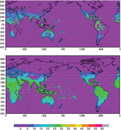
For a numerical atmospheric model, the quality of surface temperature simulation is very important as this value is an interface between the underlying medium and the atmosphere. Other characteristics of the vertical temperature profile in the underlying medium are less influential. But we would like to avoid the unrealistic profiles or drifting deep medium variables. Sometimes this may happen in the model of underlying medium, usually when using a zero thermal flux lower boundary condition. In this situation, the assimilation of observations may help. Sometimes the relaxation to climate data is applied. This problem is well known, for example, for the land surface scheme ISBA (Interactions Soil-Biosphere-Atmosphere) (Noilhan and Planton, 1989). In the lake model FLake with switched off bottom sediments module, the lower boundary condition is also of a zero thermal flux (see Mironov, 2008 for details). Hence, there is also a risk of drifting. But this does not happen in FLake for boreal freezing lakes because their temperature always reaches the maximum water density point keeping the situation stable. There is also no drift for warm shallow lakes, as they are very often mixed down to the bottom. In this situation, the bottom temperature is equal to the mean water temperature which is calculated from the bulk equation and does not drift. But for the warm deep lakes, the risk of drifting exists. Switching on the bottom sediments module unfortunately does not help here. This happens despite instead of a zero thermal flux condition on the lower boundary of the water column we have now a fixed temperature condition on the lower boundary of the new domain including bottom sediments. The reason for this is weak coupling between the water column and the bottom sediments in FLake, not enough to prevent drifting. Physically, the boundary condition on the water–sediments interface is formulated as the balance equation between fluxes of heat. Grid-point models calculate the interface (bottom) temperature from the boundary condition directly. With the self-similarity concept, the model equations primarily are integrated analytically in vertical, applying certain assumptions about the profiles of temperature and turbulent heat flux. Then they are integrated numerically in time. To couple the water column with the bottom sediments, the heat flux from the bottom sediments module is added to the prognostic equation for the bottom temperature. But the assumed profile of the heat flux in water is valid only when the mixed layer is developing, not when it is degrading. In the latter case, in FLake the bottom temperature tendency is set to zero, even with a non-zero flux from the bottom sediments. This is a shortcoming of FLake, since it is impossible with the self-similarity approach to describe accurately the very complicated bottom processes. For warm deep lakes, the following situation takes place in FLake. During night time with developing convection, the mixed layer depth increases, and the bottom temperature evolves. Normally it decreases, mainly due to the increase of the mixed layer depth and despite the heat flux from the bottom sediments, which is quite small. Then, during day time, when the mixed layer degrades, the bottom temperature in FLake remains unchanged. As a result, the bottom temperature unrealistically drifts towards the maximum water density point, this happens quite often (see Fig. 1, above). There are large territories in Africa, South America and Australia where imitative 50-m deep lakes have the unrealistic bottom temperature of 4°C. Compare with the real climatological bottom temperature in Lake Victoria (40-m deep) being approximately 24°C. In fact, the drift does not occur necessarily for all warm deep lakes. The bottom temperature evolution in FLake depends on different factors. From the atmospheric forcing side, these are annual and diurnal temperature cycles and short-wave radiation. From the lake model side, these are the lake depth and the water turbidity. Here, the turbidity parameter appears to be crucial. For example, for Lake Victoria, the problem of unrealistic bottom temperature occurs with the extinction coefficient for turbid water, but does not occur with the extinction coefficient for clear water. The behaviour of the model is very unstable at this point. This is the reason for the patchiness on Fig. 1: the problem may appear or not, depending on different combinations of forcing data and lake parameters.

To overcome this problem, we introduced a relaxation of the bottom temperature to the long-term mean screen level air temperature . We added the relaxation term to the prognostic equation for the bottom temperature in the case of degrading mixed layer:

Here t is time and τ is the relaxation time scale, h is the mixed layer depth. Zero on the right hand side of the equation stands for its form without the relaxation term. As to the equation for the case of developing mixed layer, it is not shown. It can be derived from the equations presented in Mironov (2008). The relaxation time-scale was chosen to imitate the thermal flux in bottom sediments. It is proportional to the time needed for the thermal wave to penetrate through the layer of the depth L of a medium with the certain molecular heat conductivity k (J/m/s/K), heat capacity c (J/kg/K) and density ρ (kg/m³):

As the thermal properties of bottom sediments are not known, we applied the thermal properties of water to estimate τ roughly (keeping in mind that the relaxation term is artificial). For L=0.5 m, τ≈10 d. Perhaps, for the relaxation, the deep soil temperature climatology could be applied alternatively. Theoretically, high correlations are expected between long-term mean of the bottom temperature in warm deep lakes, the deep soil temperature and the screen level air temperature. It would be interesting to study these statistics. The relaxation was only applied for deep warm lakes, which were specified as follows: these are lakes deeper than 5 m having higher than 5°C. Figure 1, below, illustrates the results. With the relaxation term applied, the bottom temperature of imitative warm deep lakes is much more realistic.

Fig. 1.  Simulated climate bottom temperature for the beginning of July for imitative lakes with 50 m depth (see text for details). Above: without a relaxation of the bottom temperature for the long-term mean screen level air temperature (note unrealistic 4 °C values for large territories in Africa, South America and Australia), below: with the said relaxation.

2.4. Projection onto the target grid

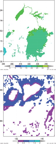
The result of climate runs is the global dataset representing the annual cycle of imitative lakes differing in terms of depth. Figure 2 illustrates the set of climate data and the system to extract information for the particular atmospheric model grid provided with the lake depth. The lake depth information may be provided by the lake database described in Kourzeneva et al. (2012). For a NWP system, climatology is usually needed on the target model grid for the specific day of the year. Normally the resolution of a target grid is finer than our 1° longitude–latitude grid. When extracting data, for each grid box of a target grid we find the grid box of our coarse grid covering it. Then, we choose the appropriate lake climate values depending on the specified lake depth in the NWP model grid box. In time, we follow the same philosophy: we find the appropriate 10-day period of the year to which the specified day belongs. Note that we do not interpolate data, as far as it is not correct for lakes. In fact, we use the method of a nearest neighbour instead. As a result, we provide the lake model climatology for any time of the year at any NWP model grid. Two examples are given by Fig. 3. First example (above) represents the vertical mean water temperature on the grid in geographical coordinates with the resolution of 0.02° for lakes in Africa including Lake Victoria, Lake Albert and small neighbouring lakes for the beginning of July. Second example (below) represents the ice depth on the grid in geographical coordinates with the resolution of 0.02° for lakes in Sweden for early January. Climate data refer to the particular date but in fact represent the appropriate 10-day interval. For both cases, the lake depth on the target grid was derived from the lake database (Kourzeneva et al., 2012). It provides the bathymetry for Lake Victoria and Lake Vanern and the mean lake depth for the smaller lakes. One can note the dependency of the lake variables on the bathymetry, e.g. most shallow lakes in Sweden are frozen, while Lake Vanern is frozen partly, deep parts are free of ice.

Fig. 2.  The set up of climate runs and the system to extract data for a particular grid of an atmospheric model provided with the lake depth. We run the lake model FLake globally on the 1° longitude–latitude grid for 20 yr with the atmospheric forcing from Sheffield et al. (2006) obtaining long-term average values (LTA). We do this 12 times as if the whole globe was covered with imitative lakes differing in depth (1 m, 3 m … 50 m). Then, we extract data for each grid box of a particular NWP model grid considering the lake depth provided.

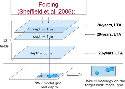
Fig. 3.  Examples of the output from the system presented in Fig. 2 (see text for details). (a) Climate field of mean water temperature, °C for July, 1, for the domain of atmospheric model in longitude–latitude coordinates with 0.02° resolution over Lake Victoria. (b) Climate field of ice depth, m for January, 1, for the domain of atmospheric model in longitude–latitude coordinates with 0.02° resolution over Sweden with Lake Vanern and partly Lake Vattern. Note different scale.

3. Validation of the results and discussion

3.1. Validation databases

Validation against independent data sources is an important part of the development permitting to estimate errors and to reveal possible problems. For validation of the lake climatology we used two independent data sources: the International Lake Environmental Committee (ILEC, 1988–1993) database, and climate data published in Ryanzhin (1989 1990 1991). Both of them include data for individual lakes around the world. Lakes differ in geographical location, elevation above sea level, size, depth, water turbidity and mineralization. These data are not harmonised, they are quite scattered in terms of time and space representation. Long-term mean values are few, often there are only data for one particular year. Sometimes there are results from measurements campaigns for specific time periods. For large lakes, measurements are performed at different stations located in different parts of the lake. We collected all this together. Thus, observational data are not accurate enough to compute the exact statistics. That is why we quantified errors in our climatology quite approximately. This appeared to be enough to reveal several problems.

3.2. General results

To examine minimum, maximum and mean values of the lake surface temperature, we used data from both datasets combined to one sample, although this is quite an inaccurate method. We used data for 99 lakes from Ryanzhin (1989 1990 1991) and for 208 lakes from ILEC (1988–1993). There are only eight lakes presented in both datasets. Temperature characteristics may differ between them up to 4°C due to various reasons, such as different averaging time periods, or different locations of hydrological stations. The results of validation for different continents are given in Table 1. Since only simple statistics are possible, we analysed the mean bias error for temperature and the biases in maximum and minimum of annual temperature cycle. For the freezing lakes, the minimum annual water temperature has no sense because it is always equal to 0°C. Thus, for the minimum water temperature we did not compute the statistics for boreal zone, we considered only Africa and Australia. In Table 1, the number of measurements for each continent is given in parenthesis. Note that not all statistics are significant. For Australia and South America, error statistics are not significant since there are little data. For these continents, we only have a rough idea about errors. Our model climatology overestimates the maximum annual surface water temperature everywhere. For Africa, where the number of measurements is enough, the bias reaches 2.5 °C. For Africa, the mean bias error is also positive and the minimum annual temperature bias is slightly negative. This means that for Africa our model climatology is warmer than in reality. For North America, there is the smallest positive bias in the maximum annual temperature, but the largest negative mean bias error (−1.1 °C). Thus, for North America our model climatology is too cold. For Europe and for Asia, there is the positive bias in maximum annual temperature but the negative mean bias error. That means that for these continents the modelled amplitude of the annual cycle is too large. This is in agreement with errors related to freeze-up and break-up dates (see Section 3.5).

Table 1. Biases between the modelling results and the measured characteristics of the annual cycle of the water surface temperature: mean, minimum and maximum values, °C

	Mean	Minimum	Maximum
Africa	1.5 (23)	0.5 (23)	2.5 (29)
North America	1.1 (34)	–	0.1 (65)
Asia	0.3 (52)	–	0.9 (74)
Europe	0.8 (48)	–	1.4 (76)
South America	2.7 (5)	1.2 (10)	3.3 (11)
Australia	0.4 (3)	0.5 (4)	3.0 (4)

In parenthesis the number of lakes with measurement is given.

We examined the water surface temperature annual cycle also qualitatively through the extensive visual comparison which allowed revealing several characteristic cases. This was done for different climate zones and for various lake types. Combining this with the analysis of the temperature profiles, we distinguished four typical situations, two for boreal lakes and two for warm lakes. Here, data only from ILEC (1988–1993) were used.

3.3. Boreal lakes

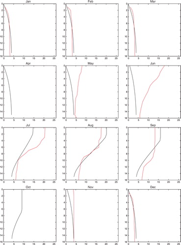
The first situation takes place for deep boreal lakes, which are dimictic or monomictic, with well pronounced temperature stratification in summer and freezing (or close to freezing) in winter. We validated our lake model climatology for 16 lakes of this type located in North America, Europe and Asia. For the Southern Hemisphere, there were no data for this lake type. Typically, for deep boreal lakes in spring in the model climatology the water surface temperature is too cold, and the temperature stratification is underestimated. In midsummer (sometimes in late summer) the situation is the opposite: the simulated water surface temperature is too high, and the temperature stratification is overestimated. In most cases, the simulated thermocline is too shallow, and the bottom temperature is too low. Thus, the modelled annual cycle is shifted and its amplitude is overestimated. The error in the water surface temperature is the highest in spring. The characteristic cases are given by Lake Amisk (North America, 15.5 m deep) and Lake Slapy (Europe, 20.7 m deep) (see Figs. 4 and 5).

Fig. 4.  Annual cycle of the water surface temperature (x-axis: time, month; y-axis: temperature, °C). Red curves – from measurements, black curves – model lake climatology.

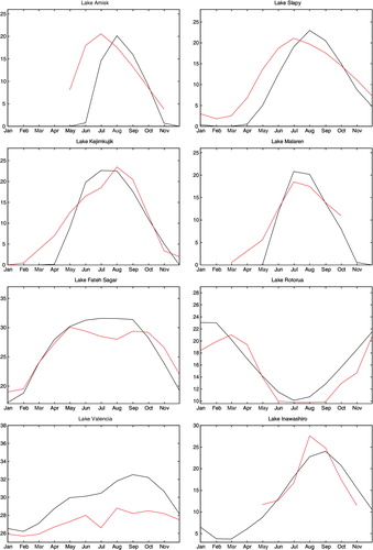
Fig. 5.  Temperature profiles in Lake Amisk (x-axis – temperature, °C, y-axis – depth, m) in different months. Red curves – from measurements, black curves – model lake climatology.

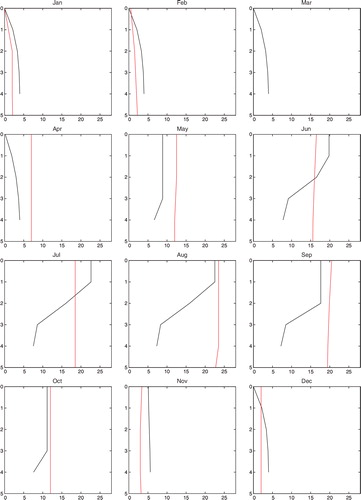
The second typical situation is associated with shallow boreal lakes, which are mainly polymictic. They are mixed almost all the year round and freeze (or being close to freezing state) in winter. For validation, data for 16 lakes of this type located in North America, Europe and Asia were available. Also here, there were no data available for the Southern Hemisphere. Typically, in spring the simulated water surface temperature for shallow boreal lakes is too cold. In early (middle) summer the simulated water surface temperature is too warm but the bottom temperature is too cold. Sometimes the undesirable vertical temperature stratification appears in the simulated profiles. In late summer or early autumn, the whole simulated profile may be shifted to lower values. Thus, the modelled annual cycle is distorted (“compressed”) and its amplitude is overestimated. However, the modelling error is much smaller for shallow lakes than for deep boreal lakes. The characteristic cases are given by Lake Kejimkujik (North America, 4.4 m deep) and Lake Malaren (Europe, 11.9 m deep) (see Figs. 4 and 6).

Fig. 6.  The same as in Fig. 5, but for Lake Kejimkujik.

3.4. Warm lakes

The third situation is connected with shallow warm lakes. They are polymictic, mixed all the year round and do not freeze during the cold season. We had very few validation data for this lake type. For the Northern Hemisphere, we had data with satisfactory quality only for two lakes in India. For the Southern Hemisphere, we had data for one lake in New Zealand. For these lakes, during the warm season, the simulated water surface temperature is too warm and the bottom temperature is too cold compared to observations. So, again the undesirable vertical temperature stratification appears. During the other seasons, this stratification may appear also, with positive or negative shift of the simulated profile. Thus, again the amplitude of the modelled annual cycle is overestimated. But the errors are essentially smaller than for shallow boreal lakes. Examples are given by Figs. 4 and 7 for Lake Fateh Sagar (Asia, 5.4 m deep) and for Lake Rotorua (New Zealand, 11 m deep). Note that in the Southern Hemisphere the cold season lasts from April to September.

Fig. 7.  The same as in Fig. 5, but for Lake Rotorua (see text for comments).

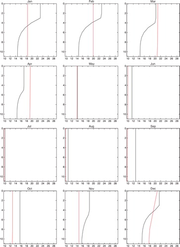
The fourth situation takes place for deep warm lakes. These lakes are non-freezing with the slight vertical temperature stratification. These are mainly monomictic lakes, but may also be polymictic or even meromictic. Note that for most of them we applied the relaxation of the bottom temperature. Data for nine lakes in Europe, Asia, Africa and North America were available for validation. For these lakes, we found no regular patterns in modelling errors both in temperature profiles and in annual cycle. Errors are smaller than for deep boreal lakes. Illustration is given for Lake Valencia (South America, 18 m deep) and for Lake Inawashiro (Asia, 37 m deep) (see Figs. 4 and 8). For Lake Valencia, the vertical temperature stratification and the annual cycle amplitude are overestimated in model climatology. For Lake Inawashiro, on the contrary, our simulation underestimates the vertical temperature stratification in summer (not shown), and thus underestimates the annual cycle amplitude.

Fig. 8.  The same as in Fig. 5, but for Lake Valencia.

3.5. Freeze-up and break-up dates

Analysis of modelling errors in freeze-up and break-up dates supports the conclusion about the shift in the simulated annual cycle for boreal lakes. We examined freeze-up and break-up dates for 91 lakes using data from ILEC (1988–1993). The mean dates of beginning and end of the ice period are usually defined with the accuracy of a month. In our research we defined these dates with the 10-day accuracy but for comparison used monthly aggregation. If, for example, the ice period starts in the end of December, we defined the freeze-up date to be in December, not in January. This may lead to an additional verification error. In our simulations, in most of the cases the ice period starts a month later than in reality. There are only a few, but very important exclusions when it starts a month earlier (for Lake Ladoga, Lake Onega and Lake Baikal). There are also 12 cases when it starts more than 1 month later, such as for Lake Superior (January vs. November, but this lake is very large and may freeze earlier in some parts). In spring, errors are much larger. There are no cases when the simulated ice period ends earlier than in reality, there are 32 cases when it ends 1 month later than in reality and in 36 cases it ends more than one month later. There are also six cases when our simulations show the ice period which is not observed in reality. Among them is Lake Vanern, which is also very large and yet may freeze in some parts.

3.6. Mountain lakes

Modelling results for mountain lakes also contain errors. Besides, point comparisons for verification very often are not correct in mountain areas. Errors come mainly from the difference in altitude between the atmospheric forcing data and the point for verification. Forcing data are represented on the 1.0° longitude–latitude grid and were designed using the reference orography on that grid. Gridded orography stands for the mean altitude value in every grid box. This may be interpreted as a kind of smoothing. When the grid box is large, its altitude may differ much from a certain point value. For example, the altitude of Lake Manasbal located in Himalaya Mountains is 1583 m. In the forcing data, the altitude (calculated from the surface pressure) of the grid box, where this lake is located, is 3960 m. The simulated maximum water surface temperature in this point is 7.7°C lower than measured. For Lake Phewa in Himalaya Mountains the situation is similar. Lake Phewa has the altitude of 742 m while the altitude of the appropriate atmospheric forcing grid box is 3570 m. The difference between the modelled and observed maximum water surface temperature is 8.5°C. But in fact, observations for Lake Manasbal and Lake Phewa can be hardly compared with the modelling results. Usually for the verification of air temperature in mountain areas, the model output is adjusted to the altitude of observations using the typical atmospheric lapse rate. But for lake temperatures, this adjustment is rather questionable because of different physics: we should consider freezing and mixing processes. For example, for the lake bottom temperature this adjustment is absolutely incorrect. Thus, in mountain areas errors are still large and difficult to handle. Users should keep in mind the difference in orography between the grid of the lake climatology dataset and the target NWP grid.

3.7. Discussion

Summarising the validation results, we may stress two main issues. First, the amplitude of the annual cycle of the water surface temperature is overestimated in many cases. Second, quite often there is a shift of the annual cycle in terms of the water surface temperature and timing of the ice period. For these errors, there may be several reasons related to different parts of our lake climate simulating system. Clearly the error may come from the lake model itself, including also a module for calculating the atmospheric surface fluxes. Lake model FLake was tested extensively (Kourzeneva and Braslavsky, 2005; Kirillin, 2010; Martynov et al., 2010; Salgado and Le Moigne, 2010; Stepanenko et al., 2010; Vörös et al., 2010 ). FLake is also widely used in different applications, including numerical atmospheric models (Mironov et al., 2010; Samuelsson et al., 2010), see also FLake website http://nwpi.krc.karelia.ru/flake/. Note that tests and validations were performed both in stand-alone mode, when atmospheric turbulent fluxes were calculated by the appropriate module in FLake, and online, when they were calculated by the host atmospheric model. However, in validation, attention was paid mainly to the water surface temperature. Timing of the ice period was less validated. For the simulated water surface temperature annual cycle, either no large errors were reported (Kirillin, 2010; Salgado and Le Moigne, 2010; Stepanenko et al., 2010; Vörös et al., 2010), or some overestimation of the amplitude was mentioned (Kourzeneva and Braslavsky, 2005; Martynov et al., 2010; Samuelsson et al., 2010). No shift in the simulated surface water temperature annual cycle was noticed. Timing of the ice period was analysed in Samuelsson et al. (2010) without mentioning significant problems. In Martynov et al. (2010), errors in timing of the ice period were reported, but in the experiments when the invalid (for FLake) lake depth was specified. In addition, the simulated freeze-up and break-up dates in their experiments were earlier than observed, while we have the opposite situation. For break-up dates, it may appear to be important that the snow module was switched off in our simulations. On the one hand, without snow, ice grows more and may disappear later. But on the other hand, ice melts faster without snow. As a result, errors may compensate each other. Testing of the snow module in FLake is ongoing (Tido Semmler, personal communications).

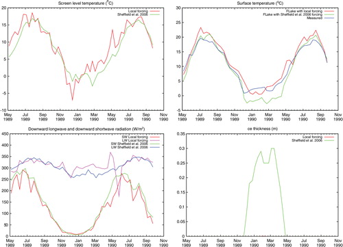
Another possible source of errors is the atmospheric forcing data. To detect these errors, an extensive comparison with other climate datasets and with in situ observations is needed. We made only one test to compare our forcing data with measurements from a campaign over Lake Erken (21 m deep) in Sweden for the period from May, 1989 to September, 1990. The same data were used in the experiments described in Kourzeneva and Braslavsky (2005). To compare with the forcing data from Sheffield et al. (2006) and with climate simulations, we averaged data from local measurements over 10-day periods (see Fig. 9 for results). Note that we excluded from the analysis the period from the end of April till the beginning of May because of problems in measurements. In winter 1989–1990, there was no ice in the simulation with the local forcing, but there was 30 cm of ice in the simulation with the forcing from Sheffield et al. (2006). Except the ice period, there is a good agreement between measured water surface temperature and simulations with different forcing data. Between different kinds of forcing, there is also a good agreement in terms of the screen level temperature and the downward short-wave radiation. But in terms of the downward long-wave radiation, there is a systematic difference of approximately 50 W m⁻² in winter period. In the forcing from Sheffield et al. (2006), there is less downward long-wave radiation, hence more ice in simulations. Thus, we may suspect errors in the atmospheric forcing to be a reason for the serious problems in our lake climate simulations, although this hypothesis should be checked further. Too rough averaging of ice data when obtaining the long-term mean values from the climate run may also enhance errors here. This was discussed in Section 2.2, and should be studied later.

Fig. 9.  Simulations for Lake Erken, Sweden, with forcing from local measurements and from Sheffield et al. (2006). Note problems with measured downward long-wave radiation in the end of April–beginning of May (see text for comments).

4. Conclusion

A dataset of model lake climatology for parameterisation of lakes in NWP was developed. This dataset may be used in NWP models to initialise prognostic variables in a lake parameterisation scheme in a case of the first, so-called “cold” start. It may be used also to prescribe the lake surface temperature in a numerical atmospheric model if no better information is available. The climatology was obtained from a 20-year run of the lake model FLake (Mironov, 2008). We run the lake model offline using the atmospheric forcing from Sheffield et al. (2006) on the global longitude–latitude grid with the resolution of 1°. We run the model several times for imitative lakes in every grid box differing in terms of the lake depth. Then, these data can be projected onto the target grid of an atmospheric model depending on the lake depth values on this grid. The advantage of this approach is a real grid-independency. The target grid may be in any coordinate system with any resolution and any form of grid cells. Since the lake model FLake uses self-similarity approach and hence does not describe accurately bottom processes in warm deep lakes, we proposed relaxation of the bottom temperature in such lakes towards the long-term mean screen level temperature. The dataset on lake climatology and the routines to project data onto the target NWP model grid will be provided for free from http://nwpi.krc.karelia.ru/flake/.

Validation of the lake climatology dataset against independent data was performed. There are no comprehensive global measurements for accurate statistics, and the existing data allow only the revealing of problems. So errors are quantified approximately. For the long-term mean and maximum water surface temperature, there is a good agreement between measured and simulated climatology. In our model climatology, there is a warm bias in Africa and a cold bias in North America. We overestimate the amplitude of the annual cycle for lakes in boreal zone as well as for warm shallow lakes. For boreal lakes, we also have a shift in the annual cycle and large errors in spring time. Related are serious errors in timing of ice period, which is lagged for this reason. Errors are smaller for shallow than for deep lakes and for warm than for boreal lakes. The reasons for the problems revealed may be connected with the lake model itself, with errors and uncertainties in forcing data, and with averaging techniques. Further study is needed to understand the relative importance of the different error sources and to make corrections where possible.

5. Acknowledgements

The authors would like to thank Dmitrii Mironov (Deutscher Wetterdienst), Bertrand Decharme, Elena Zakharova and Stephanie Faroux (Météo-France), Patrick Samuelsson and Stefan Gollvick (Swedish Meteorological and Hydrological Institute) and Laura Rontu (Finnish Meteorological Institute) for useful discussions. Two anonymous reviewers made many useful comments. The project was made possible due to the support from Météo-France.

References

- Blenckner T. Omstedt A. Rummukainen M. A Swedish case study of contemporary and possible future consequences of climate change on lake function. Aquat. Sci. 2002; 64: 171–118.
- Dirmeyer, P. A, Gao, X, Zhao, M, Guo, Z, Oki, T and co-authors. 2005. The Second Global Soil Wetness Project (GSWP-2): multi-model analysis and implications for our perception of the land surface. COLA Tech. Rep. 185, 46 pp. Online at: ftp://grads.iges.org/pub/ctr/ctr_185.pdf.
- Dutra, E, Stepanenko, V. M, Balsamo, G, Viterbo, P, Miranda, P. M. A and co-authors. 2010. An offline study of the impact of lakes on the performance of the ECMWF surface scheme. Boreal Env. Res. 15, 100–112.
- Eerola K. Rontu L. Kourzeneva E. Shcherbak E. A study on effects of lake temperature and ice cover in HIRLAM. Boreal Env Res. 2010; 15: 130–142.
- Hostetler S. Bates G. Giorgi F. Interactive coupling of a lake thermal model with a regional climate model. J. Geophys. Res. 1993; 98: 5045–5057.
- ILEC: International Lake Environmental Committee, 1988–1993. Survey of the State of World Lakes. Data Books of the World Lake Environments. Vols. 1–5. ILEC/UNEP Publications, Otsu, Japan. Data available online at: http://wldb.ilec.or.jp/.
- Kalnay E. Kanamitsu M. Kistler R. Collins W. Deaven D. Joseph D. The NCEP/NCAR 40-year reanalysis project. Bull. Amer. Meteor Soc. 1996; 77: 437–471.
- Kirillin G. Modeling the impact of global warming on water temperature and seasonal mixing regimes in small temperate lakes. Boreal Env Res. 2010; 15: 279–293.
- Kourzeneva, E and Braslavsky, D. 2005. Lake model FLake, coupling with atmospheric model: first steps. In: Fourth SRNWP/HIRLAM Workshop on Surface Processes and Assimilation of Surface Variables jointly with HIRLAM Workshop on Turbulence. P. Undèn. Workshop report, SMHI, Norrköping, Sweden, pp. 43–53.
- Kourzeneva E. External data for lake parameterization in numerical weather prediction and climate modeling. Boreal Env. Res. 2010; 15: 165–177.
- Kourzeneva, E, Asensio, H, Martin, E and Faroux, S. 2012. Global dataset for the parameterisation of lakes in numerical weather prediction and climate modelling. Tellus A, 64, 15640, DOI: 10.3402/tellusa.v64i0.15640.
- Martynov A. Sushama L. Laprise R. Simulation of temperate freezing lakes by one-dimensional lake models: performance assessment for interactive coupling with regional climate models. Boreal Env. Res. 2010; 15: 143–164.
- Mironov D. 2008. Parameterization of Lakes in Numerical Weather Prediction. Description of a Lake Model. COSMO Technical Report 11. Deutscher Wetterdienst, Offenbach am Main, Germany.
- Mironov, D, Heise, E, Kourzeneva, E, Ritter, B, Schneider, N and co-authors. 2010. Implementation of the lake parameterisation scheme FLake into the numerical weather prediction model COSMO. Boreal Env. Res. 15, 218–230.
- New M. G. Hulme M. Jones P. D. Representing twentieth-century space–time climate variability. Part 1: Development of a 1961–90 mean monthly terrestrial climatology. J. Climate. 1999; 12: 829–856.
- Noilhan J. Planton S. A simple parameterization of land surface processes for meteorological models. Mon. Wea. Rev. 1989; 117: 536–549.
- Perroud M. Goyette S. Impact of warmer climate on Lake Geneva water-temperature profiles. Boreal Env. Res. 2010; 15: 255–278.
- Ryanzhin, S. 1989. Relationships for thermal regime of freshwater lakes of the world lakes. Akad. Nauk SSSR, Inst. Ozerovedeniya, 70 (in Russian).
- Ryanzhin, S. 1990. The surface temperature of freshwater lakes in Northern Hemisphere depending on geographical latitude and elevation above sea level. Dokl. Akad. Nauk SSSR. 312( N1), 209–214. ( in Russian).
- Ryanzhin, S. 1991. Zonal distribution of thermal regime elements of lakes in Northern Hemisphere. Vodnie resursi. 4, 15–29. ( in Russian).
- Salgado R. Le Moigne P. Coupling of the FLake model to the Surfex externalized surface model. Boreal Env. Res. 2010; 15: 231–244.
- Samuelsson P. Kourzeneva E. Mironov D. The impact of lakes on the European climate as simulated by a regional climate model. Boreal Env Res. 2010; 15: 113–129.
- Sheffield J, Goteti G. Wood E. F. Development of a 50-year high-resolution global dataset of meteorological forcings for land surface modeling. J. Climate. 2006; 19(13): 3088–3111.
- Stackhouse, P. W, Gupta, S. K, Cox, S. J, Mikowitz, J. C, Zhang, T and Chiacchio, M. 2004. 12-year surface radiation budget data set. GEWEX News. Vol.14, No. 4, International GEWEX Project Office, Silver Spring, MD, 10–12.
- Stepanenko, V. M, Goyette, S, Martynov, A, Perroud, M, Fang, X and co-authors. 2010. First steps of a Lake Model Intercomparison Project: LakeMIP. Boreal Env. Res. 15, 191–202.
- Troy, T. J and Wood E. F. 2009. Comparison and evaluation of gridded radiation products across northern Eurasia. Environ. Res. Lett. 4, 045008, DOI: 10.1088/1748-9326/4/4/045008.
- Vörös M. Istvánovics V. Weidinger T. Applicability of the FLake model to Lake Balaton. Boreal Env. Res. 2010; 15: 245–254.