Dynamical influence of gravity waves generated by the Vestfjella Mountains in Antarctica: radar observations, fine-scale modelling and kinetic energy budget analysis

ABstract

Gravity waves generated by the Vestfjella Mountains (in western Droning Maud Land, Antarctica, southwest of the Finnish/Swedish Aboa/Wasa station) have been observed with the Moveable atmospheric radar for Antarctica (MARA) during the SWEDish Antarctic Research Programme (SWEDARP) in December 2007/January 2008. These radar observations are compared with a 2-month Weather Research Forecast (WRF) model experiment operated at 2 km horizontal resolution. A control simulation without orography is also operated in order to separate unambiguously the contribution of the mountain waves on the simulated atmospheric flow. This contribution is then quantified with a kinetic energy budget analysis computed in the two simulations. The results of this study confirm that mountain waves reaching lower-stratospheric heights break through convective overturning and generate inertia gravity waves with a smaller vertical wavelength, in association with a brief depletion of kinetic energy through frictional dissipation and negative vertical advection. The kinetic energy budget also shows that gravity waves have a strong influence on the other terms of the budget, i.e. horizontal advection and horizontal work of pressure forces, so evaluating the influence of gravity waves on the mean-flow with the vertical advection term alone is not sufficient, at least in this case. We finally obtain that gravity waves generated by the Vestfjella Mountains reaching lower stratospheric heights generally deplete (create) kinetic energy in the lower troposphere (upper troposphere–lower stratosphere), in contradiction with the usual decelerating effect attributed to gravity waves on the zonal circulation in the upper troposphere–lower stratosphere.

• gravity wave
• radar observation
• numerical modelling
• kinetic energy
• budget

1. Introduction

1.1. General view of the present work

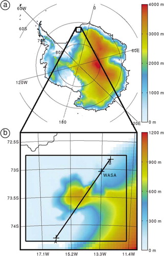
As pointed out by Fritts and Alexander (2003) in a review study, gravity waves either originating from topography, convection, wind shear, geostrophic adjustment, body forcing or wave–wave interaction significantly influence the dynamics of the atmosphere at all levels on both small- and large-scales. This is the subject investigated in the present paper for the particular case of the gravity waves generated by the Vestfjella Mountains (in western Droning Maud Land, Antarctica, southwest of the Finnish/Swedish Aboa/Wasa station located at the Basen nunatak 73°02′38″S, 13°24′26″W, see Fig. 1) during the SWEDish Antarctic Research Programme (SWEDARP) in December 2007/January 2008 (Valkonen et al., 2010). For this purpose wind observations from the Moveable atmospheric radar for Antarctica (MARA) at the Basen nunatak will be discussed, and complemented with a 2-month Weather Research Forecast (WRF; Skamarock and Klemp, 2008) model experiment coupled with European Center for Medium-Range Weather Forecasts (ECMWF) operational analyses. This model experiment will be compared with a similar one in which the orography has been removed, in order to separate unambiguously the contribution of the so-called mountain waves with respect to other synoptic processes of non-orographic origin. A kinetic energy budget analysis computed in the two simulations, with and without orography, will be presented for quantifying the role played by these mountain waves on the atmospheric flow. Some previous researches related to this topic are now reported.

Fig. 1.  (a) Terrain elevation of Antarctica. The black square shows the location of the WRF outer domain. The altitude is in metres above mean sea level with the scale given by the coloured bar on the right-side of the figure. (b) As in (a), except for the WRF outer domain and for the inner domain delimited by the black inner square, in the case of the WRF simulation with orography. The curved line on the north-west corner corresponds to the coast, the straight line (A–B) gives the location of the vertical cross-sections in Figs. 5, 9, 10 and the position of the Aboa/Wasa station at the Basen nunatak is also indicated by a cross on this line. The mountainous area crossed by A–B is the Vestfjella Mountains.

1.2. Review of past studies

In an earlier study Sawyer (1959) showed with theoretical arguments that gravity waves of orographic origin ‘dissipate energy and act as a resistance to the large-scale motion’ up to the stratosphere (Sawyer, 1959, p. 31), although he did not show the vertical distribution of this drag. Bretherton (1969) found in another theoretical work that this ‘drag acts on the synoptic scale mean flow only at just those levels where the waves are dissipated’ (Bretherton, 1969, p. 242). Studies based on field campaigns led to similar conclusions, such as that of Lilly and Kennedy (1973) who used aircraft measurements of the 1970 Colorado Lee Wave experiment to effectively associate an observed dissipation of kinetic energy around 100–200 hPa with enhanced downward flux of westerly momentum provoked by a stationary mountain wave dissipating at these levels.

The dissipation, or breaking, of gravity waves can have several origins, although the vertically propagating mountain waves that reach the upper troposphere, eventually higher levels, generally break through convective overturning (i.e. when the wave field becomes statically unstable) (e.g. Fritts and Rastogi, 1985). This process was further detailed in the theoretical work of VanZandt and Fritts (1989). In particular a gravity wave that reaches layers of increased static stability, e.g. the tropopause, is subject to an important compression of its vertical wavelength so that the wave field may become saturated and the gravity wave break. This breaking leads to an increase of turbulent energy and drag on the large-scale flow. These authors concluded that additional studies were required for really quantifying the effect of these gravity waves on the global atmosphere.

This question was then investigated with global circulation models by taking into account the known subgrid effects of these gravity waves. McFarlane (1987), among others, used for this purpose a parameterisation of orographically excited gravity wave drag to show that their breaking substantially reduce the wind speeds in and above the upper tropospheric jet of the winter northern hemisphere, thus explaining the systematic westerly bias in the general circulation models compared to the climatology.

Continuous observations by very high-frequency (VHF) radars have also been considered to study this topic. For example, Fritts et al. (1990) used a 6-d period data of the middle and upper atmosphere (MU) radar in Shigaraki, Japan, to confirm that atmospheric motions, likely gravity waves, contribute to decelerate the zonal flow in the lower stratosphere. Prichard and Thomas (1993), using a 30-month dataset from the Mesosphere-Stratosphere-Troposphere (MST) radar at Aberystwyth, Wales, also estimated the momentum flux associated with the gravity waves detected by the radar. They separated the high-frequency waves (period lower than 6 h), likely of orographic origin, from the low-frequency waves (period higher than 6 h), likely resulting from geostrophic adjustment of the jet stream, and obtained that both waves contribute similarly to this deceleration of zonal flow in the lower stratosphere. In a review study of VHF radar, Röttger (2000) highlighted that numerical modelling resolving explicitly gravity waves would be a good complement for studying their characteristics as well as for discriminating them from other long-period waves in the radar data. Indeed model analysis gives insight in the atmospheric processes while VHF radar measurements provide data at an appropriate temporal and vertical resolution to compare with the model results (e.g. Serafimovich et al., 2006; Sato and Yoshiki, 2008).

In a numerical simulation of a large-amplitude mountain wave observed over Greenland during the Fronts and Atlantic Storm-Track EXperiment (FASTEX) in January 1997, Doyle et al. (2005) showed that this wave deformed the tropopause and that its breaking at this level was associated with convective overturning layers in its field, thus suggesting that gravity waves play a role in stratospheric–tropospheric exchanges through turbulent mixing. Simulating a mountain wave observed over the Andes with the WRF model, Spiga et al. (2008) verified the mechanism originally proposed by Scavuzzo et al. (1998) that the breaking of a mountain wave in the lower stratosphere results in the emission of inertia-gravity waves (IGW, i.e. gravity waves with sufficiently low-frequency compared to the inertia frequency so that their motion is influenced by the earth rotation) that propagate further up. By comparing Microwave Limb Sounder limb-tracking 63 GHz radiance measurements and simulations with the Naval Research Laboratory Mountain Wave Forecast Model, Jiang et al. (2002) brought further evidence that mountain waves over the Andes may propagate up to 50 km altitude when tropospheric and stratospheric winds are dominated by westerlies.

Using long duration balloon flights performed during the Vorcore campaign in Antarctica (September 2005–February 2006), Hertzog et al. (2008) were able to derive momentum fluxes carried by the observed gravity waves in the lower stratosphere. They obtained predominantly westward zonal momentum fluxes, indicating that gravity waves reaching the stratosphere were mostly propagating against the mean eastward flow at these heights. Assuming the momentum fluxes measured by the balloons over mountainous areas were related to orographically generated gravity waves, they obtained that these so-called mountain waves account for two thirds of the total momentum flux over Antarctica, the nature of the non-orographic gravity waves contributing to the rest of this momentum flux remaining however undetermined. Plougonven et al. (2008) focused in particular on the large-amplitude orographic gravity wave observed on 7 October 2005 over the Antarctic Peninsula. Modelling this mountain wave with the WRF model, they showed further evidence of its breaking in the lower stratosphere due to convective overturning, in association with strong negative values of momentum fluxes in the direction of the mean flow as well as a secondary generation of IGW propagating upward in the stratosphere. With the help of ECMWF analyses, they estimated that such large-amplitude gravity wave events are present 10% of the time over the Antarctic Peninsula.

With a WRF simulation of a mountain wave observed by the ESRAD VHF radar in Esrange, Sweden, during the MaCWAVE sounding rocket campaign in January 2003, Kirkwood et al. (2010) investigated the relationship between increased turbulence and wave activity seen in the radar. The radar data were approximately reproduced in the simulation except for some details in the short time and fine vertical scales, which was attributed to the coarse temporal and vertical resolutions of the input meteorological data for the model. The simulated gravity wave was actually trapped in the lower troposphere because of increased vertical wind shear associated with a strong northwesterly jet in the mid-troposphere. The 1-km horizontal resolution in the simulation was sufficient to resolve thin wave-induced layers of convective instability in the upper region of the wave field, which certainly contributed to the turbulent mixing detected by the radar at these heights.

Valkonen et al. (2010) focused on three stationary gravity waves generated by the isolated Basen nunatak northeast of the Vestfjella Mountains (Fig. 1) during SWEDARP 2007/2008, the VHF MARA radar having been operating exactly at this location. The three gravity waves (on 9–14 December, 31 December and 12–13 January) occurred in the presence of north-easterlies in the low-levels blowing on the Basen nunatak, this wind direction being the mean annual wind direction at Aboa/Wasa (Kärkäs, 2004). WRF model simulations at 0.8 km horizontal resolution and 57 vertical levels with a top model at 50 hPa (approximately 19 km) produced gravity waves with characteristics comparable to that in the MARA data. The simulations further showed that these mountain waves generated by the Basen nunatak are well dissociated from the stronger gravity waves generated by the higher nunataks of the Vestfjella Mountains down-wind (to the southeast), and that they can propagate up to the lower stratosphere when there is not too much shear in the zonal wind.

1.3. Outlines of the present work

The present study complements the work of Valkonen et al. (2010) for the whole system of gravity waves generated by the Vestfjella Mountains during the period when MARA was doing continuous measurements in the troposphere–lower stratosphere, i.e. from 5 December 2007 to 31 January 2008. In the light of the previous researches related above we will investigate the consequences that these gravity waves had on the atmospheric dynamics up to the lower stratosphere. MARA data are analysed for the considered period in Section 2, the WRF modelling with and without orography is presented in Section 3, the kinetic energy budget analysis to quantify the influence of these gravity waves on their surrounding flow in the numerical simulation is detailed in Section 4, and some conclusions are given in Section 5.

2. Radar observations

2.1. About the instrument

MARA is an interferometric VHF radar operating at 54.5 MHz. It consists of 48 dipole-antennas arranged in three-square arrays, each with 16 dipoles spaced 4 m apart. This gives a two-way beam-width of about 9° (see Kirkwood et al., 2007, 2008; Valkonen et al., 2010, for the details). With a radar beam steered only at the vertical, MARA measures the height profile of vertical winds determined from the Doppler shift of the returned signal, as well as of the horizontal winds and rms velocity fluctuations determined by the full correlation technique (Briggs, 1984; Holdsworth and Reid, 2004). Moreover the height profile of radar echo power returned from the troposphere and lower stratosphere is supposed to depend on the distance from which the echo is returned, atmospheric density, static stability, humidity gradients and the fine-scale structure of temperature and density fluctuations within the scattering volume (e.g. Gage, 1990). In practice, for vertically pointing radars operating around 50 MHz such as MARA, the first three parameters have been found to dominate and echo power can be scaled to also provide an estimate of static stability, i.e. buoyancy frequency, especially in the upper troposphere and lower stratosphere where humidity is negligible (e.g. Kirkwood et al., 2010).

2.2. About the observed gravity waves

In December 2007/January 2008 during SWEDARP, MARA was operating at the Basen nunatak close to the Aboa/Wasa station (Fig. 1). The tropospheric and lower stratospheric measurements were done at the enhanced height resolution of 150 m (300 m) from 5 December 2007 to 1 January 2008 (from 2 to 31 January 2008), and the gravity waves observed during the whole period are now discussed.

Figure 2a–c give the time evolution of the vertical profile of vertical velocity and horizontal winds deduced from these radar measurements. Values associated with a signal-to-noise ratio lower than 0.5 have been disregarded. Figure 2a–c reveal successive events of enhanced vertical velocities associated with stronger winds, mainly between 1 and 12 km altitude. Radar measurements of wind velocities deduced from the full correlation technique are generally not available above these heights because the signal-to-noise ratio is too low at these altitudes. Figure 2a–c allowed us to identify eleven events of more or less defined vertically stacked layers of positive and negative vertical velocities associated with winds having a north-easterly component (namely north–northwesterlies, northerlies, northeasterlies, easterlies, east–southeasterlies) in the low-levels (on 5–6 December, 9–14 December, 19 December, 21–22 December, 26–27 December, 30 December–1 January, 3–5 January, 8 January, 12–13 January, 19–22 January and 25–29 January, see Table 1). Following Valkonen et al. (2010), these features are considered as the signatures of gravity waves triggered by low-level north-easterlies (at least winds having a northeasterly component) blowing on the Basen nunatak. Figure 2a–c also allow to identify five cases of gravity waves associated with low-level winds having a southwesterly component (on 18 December, 23 December, 29–30 December and 15–16 January) that all propagate up to 10 km, gravity wave excitation by southwesterlies over the Vestfjella Mountains being however disregarded in the present study.

Fig. 2.  (a–c) Time-height diagram of vertical velocity (colours) and horizontal winds (arrows) in ms⁻¹, from MARA observations. The horizontal axis gives the time in days (a: 5–23 December 2007, b: 24 December 2007–11 January 2008, c: 12–31 January 2008) and the vertical axis gives the height in m. The vertical velocity scale is given by the coloured bar on the right of each panel. The wind scale is given by the arrow above this coloured bar. (d–f) As in (a–c), except from the WRF inner model experiment with orography.

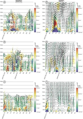
Table 1. Occurrence of tropospheric gravity waves associated with low-level winds having a northeasterly component, as inferred with MARA data during the period from 5 December 2007 to 31 January 2008. The first column indicates the days when the gravity wave was detected, the second column gives the time duration of the event in hours, the third column gives the highest height reached by the low-level winds having a northeasterly component and the fourth column the highest height reached by the gravity wave. Gravity waves reaching tropopause heights are in bold characters

Date	Duration (h)	Highest altitude reached by the low-level winds having a northeasterly component (km)	Highest altitude reached by the gravity wave (km)
5–6 December	48	3	4
9–14 December	144	11	12
19 December	24	10	10
21–22 December	24	3	14
26–27 December	36	11	11
30 December–1 January	48	8	12
3–5 January	48	11	11
8 January	12	2	5
12–13 January	48	8	12
19–22 January	120	4	4
25–29 January	120	10	10

Coming back to the gravity waves associated with low-level northeasterlies, four cases (5–6 December, 21–22 December, 8 January and 19–22 January) are characterised by winds with a northeasterly component confined in the lower levels and in general no vertical propagation above 4 km altitude. The case of 21–22 December is an exception to this since it is associated with winds veering to southerlies above 3 km but enhanced vertical velocities are detected up to 14 km.

The seven other cases (9–14 December, 19 December, 26–27 December, 30 December–1 January, 3–5 January, 12–13 January and 25–29 January) are on the contrary associated with winds having a northeasterly component up to 8–11 km altitude, and all of them show some gravity wave activity in the upper troposphere/lower stratosphere (see in Fig. 2a–c the enhanced positive vertical velocities around 10 km for these events). Generalising the conclusion of Valkonen et al. (2010) to all the cases considered here, omitting the case of 21–22 December, we attribute this (non-) propagation up to the lower stratosphere to reduced (enhanced) wind shear associated with upper-level winds having a southwesterly component.

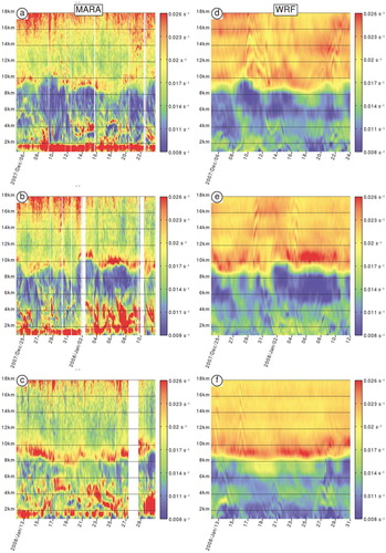
Mountain waves reaching tropopause heights may induce convective instability layers and consequently break (e.g. Fritts and Rastogi, 1985; Doyle et al., 2005). This point, in relation with the upper-tropospheric/lower-stratospheric wave activity previously discussed, is now investigated with the vertical profile of radar-derived buoyancy frequency (Fig. 3a–c), humidity effects on radar measurements being negligible at these heights (e.g. Kirkwood et al., 2010). The main feature revealed by this profile is actually the fluctuation of tropopause heights between 8 and 10 km, in association with upper-tropospheric fronts crossing the volume probed by the radar. Concerning the previously discussed lower-stratospheric wave activity there is however no related feature in the buoyancy frequency field that can be clearly identified in Fig. 3a–c, except for the case of 9–14 December (see in Fig. 3a the hints of elongated tilted strips of weaker and stronger static stability between 10 and 16 km altitude during that period). This suggests that only this case was intense enough to induce some fluctuations in the static stability field, although the lowest values detected by the radar are not those of convective instability layers. The radar data alone do not give much more information concerning the physics associated with this feature. Gravity waves generated by the Basen nunatak are actually part of a larger system of gravity waves over the Vestfjella Mountains (Valkonen et al., 2010, Fig. 1) and the phenomenon certainly has to be considered in its globality for properly understanding these radar observations. As pointed out by Serafimovich et al. (2006) or Sato and Yoshiki (2008), physical processes associated with radar-observed phenomena can be further investigated with model analysis. This is what we propose to do in the following section.

Fig. 3.  As in Fig. 2, except for the buoyancy frequency (s⁻¹).

3. Numerical simulation

3.1. Setting of the experiment

Valkonen et al. (2010) showed that gravity waves generated by the Basen nunatak during SWEDARP 2007/2008 are correctly reproduced in 4-d WRF simulations at 0.8 km horizontal resolution using 57 vertical levels up to approximately 19 km (50 hPa), according to the MARA observations. We propose here to conduct a similar numerical simulation from 5 December 2007 to 31 January 2008 when MARA was continuously operating, and for a larger domain encompassing the whole Vestfjella Mountains since we are interested in studying the whole system of gravity waves generated in this area. A control experiment without orography is also conducted in order to separate unambiguously the contribution of these mountain waves with respect to other synoptic processes of non-orographic origin.

More precisely the two simulations, with and without orography, presented here consist of two nested polar stereographic domains at horizontal resolutions 6 and 2 km (Fig. 1b), with 95 vertical levels up to 20 hPa (approximately 25 km). The vertical spacing is stretched from 60 to 350 m at the lowest and highest level, respectively. Rayleigh damping in the uppermost 5 km was introduced in order avoid spurious wave reflection from the model lid (following Durran and Klemp, 1983). For the simulation with orography, the terrain elevation of the inner model is specified by the data from the Radarsat Antarctic Mapping (RAM) Project Digital Elevation (PDE) Model Version 2 originally at 1 km resolution (Liu et al., 2001). The two numerical experiments start 1 d before the period of interest at 0000 UTC 4 December 2007 and are run for 58 d. They are coupled with ECMWF operational analyses at the initial time and every 6 h at the boundaries of the outer domain. The model equations are integrated in the outer and inner domains at time steps of 24 and 8 s, respectively. The inner model outputs containing the usual dynamic and thermodynamic variables, as well as the terms of the kinetic energy budget presented in Section 4, are then saved every hour.

Convection is explicit in the inner and outer domains and microphysics is parameterised with the three-class liquid and ice hydrometeors scheme of Hong et al. (2004). Radiative processes are represented with the long and short-wave radiation schemes of Mlawer et al. (1997) and Dudhia (1989), respectively. Subsurface heat conduction was calculated with a scheme based on a five-layer snow temperature, and the turbulent transport of heat, moisture, and momentum was parameterised in the whole atmospheric column with the scheme of Hong et al. (2006).

3.2. Qualitative results

3.2.1. Comparison with radar measurements.

Vertical profiles similar to those deduced from the radar measurements (Figs. 2a–c and 3a–c) but computed with the outputs from the modelling experiment with orography are displayed in Figs. 2d–f and 3d–f, respectively. A comparison between the vertical profiles of vertical velocity and horizontal winds obtained from MARA and WRF data (Fig. 2) reveals two striking differences. First the model displays the strong stratospheric winds above 12 km altitude that were absent in the radar measurements due the low signal-to-noise ratio at these heights. Second the radar-deduced vertical velocities are generally much stronger than the simulated ones, which may be related to coarse model inputs, not high enough horizontal or vertical resolution, or not sufficiently resolved topography. However, the 11 gravity wave events previously described (Section 2.2) all have a signature in the simulation, with generally better defined vertically stacked layers of positive and negative vertical velocities since there is noise in the radar data that is not present in the simulation.

A comparison between the vertical profiles of buoyancy frequency obtained from MARA and WRF data (Fig. 3) shows that the main feature revealed by these profiles, i.e. the fluctuations of tropopause heights, is approximately well reproduced in the simulation. The anomalously high radar-deduced buoyancy frequency values in the lower to mid-troposphere, in comparison to the simulated ones, should be disregarded since humidity affects radar measurements at these heights. It is then comfortable to verify that the radar-deduced lower-stratospheric elongated tilted strips of weaker and stronger static stability associated with the case of 9–14 December are also visible in the simulated data at approximately the same heights and time (compare Fig. 3a,d), which means that the analysis of the modelled data will allow us to investigate the physical processes associated with this observed feature. We finally notice five other short events of lower stratospheric gravity wave activity (on 21–22 December, 30 December, 4 January, 12 January and 15–16 January) that are not clearly visible in the radar data in Fig. 3, although wave features can be seen in high-resolution plots of the radar data on 21–22 December, 29 December, 4 January and 12 January (not shown). Two of them (29 December and 15 January) are associated with gravity waves in the troposphere triggered by low-level southwesterlies blowing on the Basen nunatak (Fig. 2e,f), and for this reason are disregarded in the present study. The three others are associated with the cases of 21–22 December, 3–5 January and 12–13 January that reached tropopause heights. Thus the model suggests that these three cases as well were strong enough to induce some fluctuations in the static stability field, such as that of 9–14 December.

3.2.2. About the orographic wave of 9–14 December 2007.

We are particularly interested in the results from the modelling experiment with orography for the case of 9–14 December, since it is the strongest event of the period and the associated lower stratospheric gravity wave activity observed by the radar and reproduced in the model still has to be clarified. The 3-D structure of the gravity waves generated by the Vestfjella Mountains during this event can be inferred with the horizontal and vertical cross-sections of vertical velocity on 10 December 2007 at 21:00 UTC in Figs. 4a,b and 5a.

Fig. 4.  Result of WRF modelling experiment with orography showing the horizontal cross-section at 6000 m altitude of vertical velocity (colour) and horizontal winds (arrows) in ms⁻¹, on 10 December 2007 at 21:00 UTC. The vertical velocity scale is given by the coloured bar on the right side of the panel. The wind scale is given by the arrow on the bottom right corner of the panel. (b) As in (a), except at 16 000 m altitude.

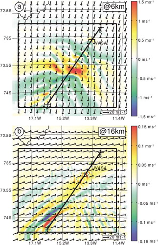
As claimed by Valkonen et al. (2010), the mountain wave at Basen nunatak is indeed part of a large system of gravity waves that extend over the whole Vestfjella Mountains up to the tropopause, with north-northeasterlies blowing up to these heights as well. The horizontal wavelength of the whole system in the troposphere is not constant with space and varies between 15 and 70 km, but its direction follows approximately that of the wind. The vertical wavelength is not constant as well, although it seems to vary between two discrete values: either the troposphere's height or half of it. It is noticeable that the most intense gravity wave activity occurs near the centre of the Vestfjella Mountains (compare Figs. 1b, 4a and 5a).

This tropospheric gravity wave is capped by a lower-stratospheric gravity wave with different characteristics (Fig. 4b and 5a). In particular this lower stratospheric wave has a smaller horizontal wavelength varying between 15 and 50 km with a direction following the westerlies at these heights, as well as a smaller vertical wavelength of about 2–3 km. The 1-h snapshots of vertical profiles of vertical velocity such as in Fig. 5a (not shown) suggest that this lower stratospheric wave emanates from the most intense peak of the tropospheric mountain wave near the centre of the Vestfjella Mountains. According to these model results we suggest that this lower stratospheric wave corresponds to the wave-like feature observed around 10 km altitude in the MARA data (compare Fig. 2a,d and 5a).

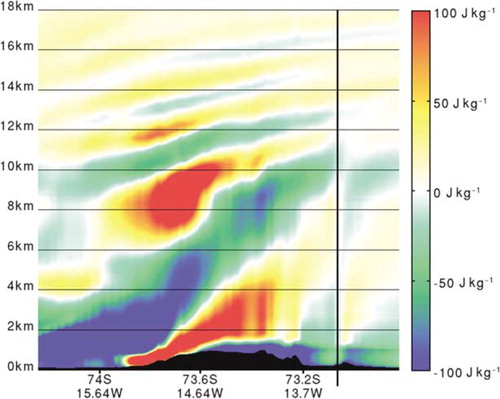
Fig. 5.  (a) Result of the WRF modelling experiment with orography showing the vertical cross-section from the inner model on 10 December 2007 at 21:00 UTC at the location indicated by the line (A–B) in Figs. 1 and 4, for the vertical velocity (colour) in ms⁻¹, the wind projected on the plane of the cross-section (arrows) in ms⁻¹ and the isentropes (black contours) in K. The horizontal axis gives the horizontal coordinate in (latitude, longitude) and the vertical axis on the left side (right side) gives the altitude in m (the potential temperature in K). The profile of the Vestfjella Mountains is shaded in black, with the Basen nunatak at the radar location indicated by the black vertical line. The vertical velocity scale is given by the coloured bar on the right side of the panel. The projected wind takes into account the vertical velocity and the scale is given by the arrows on the top right corner of the panel. (b) As in (a), except for the buoyancy frequency in s⁻¹. (c) As in (a), except for the bulk Richardson number. (d) As in (a), except for the horizontal wind orthogonal to the plane of the vertical cross-section in ms⁻¹.

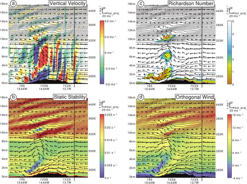
The vertical cross-section of buoyancy frequency on 10 December 2007 at 21:00 UTC (Fig. 5b) shows layers of negative static stability between 10 and 14 km, indicating that the whole system of gravity waves generated by the Vestfjella Mountains is breaking through convective instability in the lower stratosphere at this time (following the point of view of Fritts and Rastogi, 1985). This breaking is also associated with enhanced turbulence diagnosed with the bulk Richardson number in Fig. 5c, a result already claimed theoretically by VanZandt and Fritts (1989) and modelled in some case-studies (e.g. Doyle et al., 2005; Kirkwood et al., 2010). The vertical cross-section of the horizontal wind orthogonal to the projection (Fig. 5d) reveals some vertical oscillations in phase with the lower stratospheric wave discussed above, indicating that this wave is actually an IGW. The signature of this wave is also visible in the vertical cross-section of buoyancy frequency, thus explaining the origin of the wave pattern seen in the radar profiles at these lower stratospheric heights (compare Figs. 3a,d and 5b). We suggest here that this IGW results from the breaking of the orographically-induced gravity wave in the troposphere, as proposed theoretically by Scavuzzo et al. (1998), and observed by Spiga et al. (2008) or Plougonven et al. (2008). Similar vertical profiles for the whole simulated period (not shown) show that some of the previously discussed short events of lower-stratospheric gravity wave activity (on 29 December and 4 January) are also associated with tropospheric wave breaking events.

3.2.3. Box-averaged analysis.

In order to further analyse the gravity waves generated at the Vestfjella Mountains, we compute the vertical profile of the difference between the vertical velocities from the modelling experiments with and without orography, averaged horizontally in the inner domain referred to as D2 (Fig. 6a). The retrieval of the vertical velocity from the modelling experiment without orography is assumed to remove the contribution from synoptic processes of non-orographic origin, so the profile of this so-called differential vertical velocity displays only the features associated with mountain waves or other processes of orographic origin. Because D2 encompasses roughly the horizontal extension of the gravity wave generated by the Vestfjella Mountains in the modelling experiment with orography (see Fig. 3a), the time evolution of the vertical profile of D2-averaged differential vertical velocity (Fig. 6a) diagnoses this gravity wave activity during the period considered. According to Fig. 6a, all of the eight gravity waves triggered by low level northwesterlies at the Basen nunatak that reached tropopause heights (cf. Table 1) are associated with vertically stacked layers of positive and negative D2-averaged differential vertical velocities up to 8 km. The gravity waves triggered by southwesterlies on 23 December and 29–30 December are also associated with such D2-averaged vertical velocities. This suggests that these particular mountain waves were strong enough to have some impact on the atmospheric circulation at this scale. Moreover four cases triggered by northwesterlies (on 9–14 December, 21–22 December, 30 December–1 January and 3–5 January) and two cases triggered by southwesterlies (on 23 December and 29–30 December) are associated with some D2-averaged vertical velocity in the lower stratosphere strong enough to be seen in Fig. 6a, indicating some gravity wave activity at these heights as well.

Fig. 6.  (a) Time-height diagram of the difference between the vertical velocities (ms⁻¹) from the WRF model experiments with and without orography, averaged horizontally in the inner domain at a time resolution of 1 h. The horizontal axis gives the time in days from 5 December 2007 to 31 January 2008 and the vertical axis gives the height in m. The vertical velocity scale is given by the coloured bar on the right side of the panel. (b) As in (b), except for the horizontal divergence in s⁻¹. (c) As in (a), except for the difference between geostrophic and vertical relative vorticities in s⁻¹.

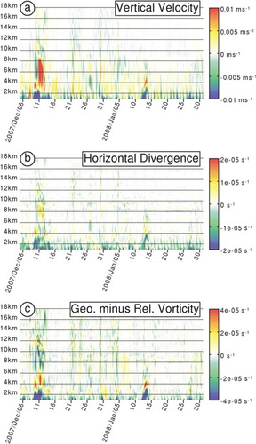
It is noticeable that Fig. 6a also displays diurnal oscillations of vertical velocity in the low levels during the whole simulation, suggesting the Vestfjella Mountains have some influence on the diurnal cycle. This feature is however not further investigated since it is not correlated with the gravity wave activity.

The time evolution of the D2-averaged vertical profile of the so-called differential horizontal divergence (Fig. 6b), between the two modelling experiments with and without orography, also shows some more or less defined wave-like pattern that can be associated with almost all the gravity waves previously described. This means that these gravity waves in general create some diverging circulation, which corresponds to a geostrophic imbalance that consequently has an impact on the large-scale circulation through geostrophic adjustment.

In order to diagnose the geostrophic imbalance induced in the flow we compute the difference between geostrophic vorticity ξ _g (eq. (1)) and relative vertical vorticity ξ, these two quantities being equal in case of a strictly geostrophic flow.1

And more precisely, in order to diagnose the particular geostrophic imbalance induced by the gravity waves we compute the vertical profile of the difference of this quantity (ξ _g −ξ) between the two modelling experiments with and without orography, averaged horizontally in the inner domain referred to as D2 (Fig. 6c). Fig. 6c confirms the previous result that most of the waves induced some ageostrophic circulation in the troposphere and in some cases in the lower stratosphere, the case of 9–14 December being the most intense. We therefore suggest that this particular case had the most important impact on the large-scale flow up to the lower stratosphere. In the following section we propose to compute the kinetic energy budget of the simulated atmospheric flow in D2 for the two modelling experiments with and without orography, in order to quantify the influence of the gravity waves generated inside D2 on the surrounding flow during the considered period.

4. Kinetic energy budget analysis

4.1. Concept

Previous studies focused on the vertical divergence of horizontal momentum fluxes induced by gravity wave motions to show their decelerating effect on the zonal circulation in the upper troposphere–lower stratosphere (e.g. Lilly and Kennedy, 1973; McFarlane, 1987; Fritts et al., 1990; Prichard and Thomas, 1993; Hertzog et al., 2008; Plougonven et al., 2008), although the sign of this divergence is negative (positive) for decelerated westerlies (easterlies), respectively. We therefore find it more appropriate to consider the vertical divergence of horizontal kinetic energy fluxes, this term being systematically negative when the horizontal flow is decelerated.

The temporal variations of this horizontal kinetic energy defined as KH=(u ²+v ²)/2, where u and v are the zonal and meridional components of the wind, may be related to the vertical divergence of its fluxes, but also to some other processes. This can be investigated with the following prognostic equation in its flux form:2

where ρ and ρ _d are the moist and dry air densities, p the atmospheric pressure, w the vertical velocity, F _x and F _y the zonal and meridional components of the frictional forces, ∂ the partial derivate with respect to time t or one of the Cartesian coordinates x, y, z. In eq. (2) the tendency of ρ _d ·KH (2a) is the sum of the horizontal and vertical divergences of ρ _d ·KH fluxes (2b and 2c), the work of pressure forces (2d) and the frictional dissipation (2e). Averaging eq. (2) in a horizontal domain: (2a) gives the time evolution of ρ _d ·KH for the flow inside the domain; (2b) gives the amount of ρ _d ·KH exchanged horizontally between the inner and outer flows; (2c) gives the amount of ρ _d ·KH transported vertically by large- and fine scale processes, gravity waves being one of them; (2d) gives the energetic impact of the ageostrophic circulation on the entire horizontal flow inside the domain; and (2e) gives the amount of ρ _d ·KH dissipated by frictional processes, mainly in the boundary layer. Such a budget of ρ _d ·KH computed for an appropriate spatial domain would therefore allow quantifying the energetic impact of a gravity wave on its surrounding horizontal flow. In the following section we propose a method to compute this budget in the WRF model.

4.2. Method

Although the WRF model is a fully compressible non-hydrostatic atmospheric model, the quantity ρ in eq. (2) is replaced by µ, the mass of the dry air per unit area within the column in the model domain at (x, y) (Skamarock and Klemp, 2008). We therefore decide to compute eq. (2) in its advective form in order to remove ρ from the equation:3

where all the quantities have already been defined except for α=1/ρ, the specific volume of the moist air. The main difference between eqs. (2) and (3) is that in eq. (3) the divergence of ρ _d ·KH fluxes is replaced by the advection of KH. Averaging this advection in a box does not strictly give the amount of KH exchanged between the inner and outer flows, although we neglect this difference in the following sections.

The terms of eq. (3) are integrated each time step during the simulation and are saved in the output files every hour as 3-D fields. It is then possible to average these terms in any box for any time-period multiple of 1 h. This allows doing a budget at a particular location as well as visualising the source and tendency terms on horizontal and vertical cross-sections in order to better localise the processes quantified in the box-averaged budget analysis.

The computation of eq. (3) in the WRF model, especially the horizontal and vertical components of advection in a terrain following coordinate system, is detailed in the Appendix. Because the numerical formulation used for computing eq. (3) is not strictly equivalent to that used in the WRF model, the obtained budget is not exactly equilibrated at grid points, which is why we always compare the tendency to the sum of the source terms when discussing the results in the following sections.

In order to separate unambiguously the contribution of mountain waves on its surrounding horizontal flow from that of other synoptic processes of non-orographic origin, we compute for each term of eq. (3) the difference of the results obtained in the two simulations with and without orography.

4.3. Results

In the following discussion we will only consider the cases of the eight gravity waves triggered by northwesterlies over the Vestfjella Mountains that are associated with vertically stacked layers of positive and negative D2-averaged differential vertical velocities up to 8 km (on 9–14 December, 19 December, 21–22 January, 26–27 December, 30 December–1 January, 3–5 January, 12–13 January and 25–29 January, cf. Table 1 and Fig. 7). Moreover the time-height plots shown in this section are computed at the time resolution of 24 h instead of 1 h as in previous sections, in order to remove the diurnal cycle detected in Fig. 6.

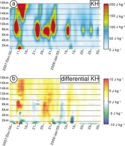
Fig. 7.  (a) As in Fig. 6, except for KH (J kg⁻¹) from the WRF simulation with orography and with a time resolution of 24 h for the input data. (b) As in (a), except for the difference of KH between the two simulations with and without orography.

4.3.1. Box-averaged horizontal kinetic energy.

A preliminary step to study the dynamical influence of gravity waves generated by the Vestfjella Mountains is to look at the D2-averaged KH. Fig. 7a displays the time evolution of its vertical profile obtained from the WRF simulation with orography. It shows enhanced values around 6–12 km (on 8–12 December, 21–23 December, 26–30 December, 31 December–3 January, 9–11 January, 20 January and 25 January), more or less accompanied by smaller maxima in the lower troposphere (1–4 km). These features correspond to the passage near D2 of upper tropospheric ridges in the westerlies overhanging lower tropospheric troughs, as inferred by snapshots of ECMWF analysis every 6 h (not shown). It is actually these lower tropospheric troughs that cause the northerlies/north-easterlies blowing over the Basen nunatak during the periods of mountain wave activity discussed in this study. It is noticeable here that the strongest low-level flow occurs during 9–14 December, simultaneously with the most intense mountain wave. A strong low-level flow, although for a shorter period, also occurs during the event of 12–13 January. The maxima of KH at heights 12–18 km are then attributed to the lower stratospheric jet moving southward closer to D2, as inferred by snapshots of ECMWF analysis (not shown).

In order to quantify the impact of gravity waves on this D2-averaged KH, the time evolution of the D2-averaged vertical profile of differential KH, between the two modelling experiments with and without orography, is displayed in Fig. 7b. It shows values of magnitude's order ±10 J kg ¹ at approximately heights and times when previously described gravity waves are propagating. The physical meaning of this value can be understood by considering for example a background wind of 10 ms⁻¹, i.e. a KH of 50 J kg⁻¹, so a variation of ±10 J kg⁻¹ in KH corresponds in this case to a variation of about ±1 m s ¹ in the background wind.

Most of the gravity waves’ cases are characterised by a decrease of KH in the low-levels, except on 8–10 December, 26–27 December and 30 December where an increase is observed. When the low-level increase occurs it is noticeable that the increase actually takes place in the whole atmospheric column up to 18 km. Otherwise the low-level decrease of KH is always capped by some increase up to 18 km, the altitude of sign's change varying from case to case (6 km on 11 December, 3 km on 12–14 December, 11 km on 19 December, 10 km on 21–22 December, 3 km on 31 December–1 January, 2 km on 3–4 December, 10 km on 5 January, 6 km on 12–13 January and 1 km on 25–29 December). In other words these particular gravity waves generated by the Vestfjella Mountains mainly decelerated (accelerated) the atmospheric flow in the lower troposphere (upper troposphere–lower stratosphere). This is somewhat contradictory to previous studies emphasising on the decelerating effect of gravity waves on the zonal circulation in the upper troposphere–lower stratosphere (e.g. Lilly and Kennedy, 1973; McFarlane, 1987; Fritts et al., 1990; Prichard and Thomas, 1993; Hertzog et al., 2008; Plougonven et al., 2008). Although these results were only based on the vertical divergence of horizontal momentum fluxes induced by gravity wave motions, which is only a proxy for the vertical advection term in the budget of KH. An detailed analysis of all the terms of this budget should be investigated to better understand the effect of gravity waves on the atmospheric flow.

4.3.2. Box-averaged budget analysis.

It was shown in previous subsection that the gravity waves generated by the Vestfjella Mountains did have some influence on its surrounding flow by modifying the D2-averaged KH. The physical processes involved in these variations can further be investigated with the temporal variations of the D2-averaged vertical profiles of the terms of the prognostic eq. (3) applied to the differential KH (Fig. 8).

Fig. 8.  As in Fig. 6, except for the difference of the terms (in W kg⁻¹) of the budget of KH between the two simulations with and without orography and with a time resolution of 24 h for the input data: (a) tendency, (b) sum of the source terms, (c) horizontal advection. (d) vertical advection, (e) horizontal work of pressure forces, (f) frictional dissipation.

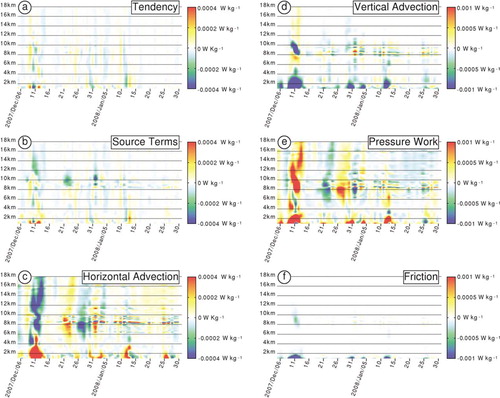
To begin with, a comparison between the tendency of differential KH (Fig. 8a) and the sum of the source terms (Fig. 8b) shows that the budget is roughly well equilibrated when averaged in D2, except some spurious negative values in the sum of the source terms around tropopause and lower stratospheric heights. The numerical approximation of the advection terms (cf. Appendix) is indeed expected to give the less accurate results when the winds are strongest. On the other hand the tendency of differential KH is much smaller than each of the source terms (Fig. 8), which means that the respective signs and orders of magnitude of these ones are well estimated, variations of the differential KH being in fact the result of small imbalances between these source terms.

The budget of differential KH is now analysed. In all gravity waves’ cases (except on 8–10 December, 26–27 December and 30 December) the low-level decrease of KH is due to dissipation by friction and negative vertical advection (Fig. 8f,d) counterbalanced by positive horizontal pressure work and horizontal advection (Fig. 8c,e). It is noticeable that when low-level increase occurs (on 8–10 December, 26–27 December and 30 December) these terms have the same signs although the imbalance is positive instead of being negative. This result can be interpreted as the following. The vertical gradient of KH is mainly negative in the low levels because of the low-level wind surges triggering the gravity waves (Fig. 7a). More over these gravity waves mainly induce negative vertical velocities in the low levels, as deduced from Fig. 6a. This up-gradient vertical flow consequently leads to negative vertical advection in the low levels. These gravity waves also increase the subgrid momentum fluxes in the boundary layer due to enhanced vertical velocities, resulting in frictional dissipation. Both these processes generate a non-geostrophic flow characterised in this case by a positive horizontal pressure work. This departure from the geostrophic equilibrium is also accompanied by some energy exchanges with the outer flow, which in this case happens to be a gain of energy as diagnosed by the positive horizontal advection. The sign of these horizontal pressure work and horizontal advection is however not explained here, and it is questionable whether it should always be positive in this case.

The upper-level increase on the other side is mainly the result of an imbalance between horizontal pressure work and horizontal advection, the sign of these terms changing from case to case, height and time, vertical advection being generally much weaker and frictional dissipation completely negligible. This means that this upper-level differential KH is mainly driven by some ageostrophic circulation inducing a horizontal pressure work and KH exchanges between the outer and inner flow. This ageostrophic circulation is certainly a consequence of the lower-stratospheric gravity waves, although this does not give any constraint on the respective sign of these horizontal pressure work and horizontal advection neither on their sum.

A special attention is addressed to the case of 8–14 December at 8–12 km where the wave is breaking (Section 3.2.2, Fig. 6b). Indeed at these heights the vertical advection is strongly negative (Fig. 8d), in coherence with the usual atmospheric drag generally accompanying the gravity wave breaking in the lower stratosphere (e.g. Lilly and Kennedy, 1973; VanZandt and Fritts, 1989; Plougonven et al., 2008). There is also some frictional dissipation at these heights (Fig. 8f), which means that this gravity wave also increases the subgrid momentum fluxes at the breaking heights where it generates turbulences (as deduced from Fig. 5b,d, and as originally proposed by VanZandt and Fritts, 1989). However, these negative terms are partially balanced by the positive sum of a negative horizontal advection (Fig. 8c) and positive horizontal pressure work (Fig. 8e), so the differential KH still decreases on 10 December (Fig. 8a) but does not become negative (Fig. 7b). The apparently contradictory upper-level increase of this differential KH is in fact reduced at breaking heights. This result clearly shows that the effect of gravity wave's breaking on the atmospheric flow cannot be inferred with the vertical advection term only.

4.3.3. Vertical cross-section analysis for the case of 9–14 December 2007.

As suggested in Section 4.2 the physical processes quantified in the horizontally averaged budget previously analysed can be localised more precisely by visualising cross-sections of the different terms. This is what we propose to do here for the particular case of 10 December 2007 at 21:00 UTC when the gravity wave starts to break (Fig. 5b). To begin with let's consider the vertical cross-section of the differential KH computed on 10 December 2007 at 21:00 UTC (Fig. 9). It shows that the gravity wave at this time induces locally much stronger deviations of KH compared to what is obtained from the D2-averaged analysis (compare Fig. 7b and 9), i.e. over ±100 J kg⁻¹ in the whole tropospheric column near the centre of the Vestfjella Mountains where the gravity wave is most intense (Figs. 4a and 5a). And KH variations induced by this particular gravity wave are more complex than what was found previously since it locally increases and decreases in the low levels, although the D2-averaged analysis only gives a slight decrease at this time (compare Figs. 7b and 9). Fig. 9 finally reveals wave-like pattern of KH in the lower stratosphere characterising the IGW triggered at these heights.

Fig. 9.  As in Fig. 5, except for the difference of KH between the two simulations with and without orography in J kg⁻¹, computed on 10 December 2007 21:00 UTC.

The physical processes involved in these variations are now investigated with the vertical cross-sections of the terms of the prognostic eq. (3) applied to the differential KH, computed on 10 December 2007 between 20:00 and 22:00 (Fig. 10). To begin with, a comparison between the tendency of differential KH (Fig. 10a) and the sum of the source terms (Fig. 10b) shows that the budget is not so well equilibrated at grid-points, especially in the boundary layer and at tropopause heights. The residual term in the budget is essentially introduced by the horizontal and vertical advection terms whose numerical computation is not equivalent to what is done in the WRF model (cf. Appendix). This means in particular that even if the order of magnitude of the frictional dissipation term (Fig. 10f) is smaller than that of the residual term, its values can still be interpreted physically because it is exactly what is computed in the model.

Fig. 10.  As in Fig. 5, except for the difference of the terms of the budget of KH between the two simulations with and without orography in W kg⁻¹, computed on 10 December 2007 between 20:00 and 22:00 UTC.

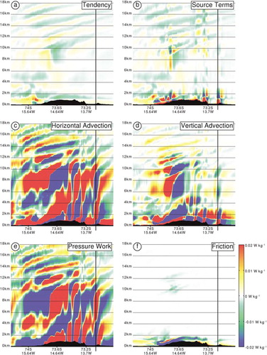
Compared to the box-averaged results, the horizontal advection at grid-points (Fig. 10c) is one to two orders of magnitude greater than its box-averaged values previously discussed (the scale in Fig. 10 has actually been saturated so that the smaller amplitude frictional dissipation can also be visualised on the same figure), and it is mainly in phase-opposition with the horizontal work of pressure forces (Fig. 10e) for the whole profile. The vertical advection (Fig. 10d) also contributes significantly to this equilibrium in the troposphere. These three source terms have wave-like features that result from the gravity wave they originate from (compare Fig. 10c–e with Fig. 5a) and it is their disequilibrium that mainly rules the variations of differential KH (Fig. 10a). The profile of differential KH in Fig. 9 cannot however be explained by the profiles of these three terms in Fig. 10, since it is actually the result of an integration of the previous variations of these three terms. The frictional dissipation (Fig. 10f) has then values of about one order greater than what was found in the box-averaged analysis, still much weaker than the three other source terms, and is localised in the low levels over the Vestfjella Mountains as well as at lower-stratospheric heights where the wave is breaking (compare Figs. 5b,c and 10f).

The tendency of KH (Fig. 10a) shows that KH is actually depleted above the Vestfjella Mountains between 7 and 12 km on 10 December 2007 between 20:00 and 22:00, and a comparison with Fig. 10b suggests that this depletion can be explained by the sum of the source terms. The budget analysis further shows that this depletion of KH between 7 and 12 km is the result of a negative imbalance between three vertically stacked positive and negative layers of horizontal advection/horizontal pressure work in phase opposition, three other vertically stacked positive and negative layers of vertical advection with a different phasing and frictional dissipation. It is finally noticeable that this depletion of KH at this time and heights is also visible in the D2-averaged analysis (see Fig. 8a).

5. Conclusion

During the SWEDARP expedition that was held at the Finnish/Swedish Aboa/Wasa station in December 2007/January 2008, radar measurements were operated with the MARA VHF radar at the Basen nunatak, northeast of the Vestfjella Mountains. For the period from 5 December 2007 to 31 January 2008 in particular, MARA was making continuous tropospheric and lower stratospheric measurements at the enhanced height resolutions of 150 and 300 m. Vertical profiles of vertical velocities and horizontal winds deduced from these radar data showed the signature of 11 tropospheric gravity waves in the presence of enhanced winds having a northeasterly component at low levels. Following Valkonen et al. (2010), these tropospheric waves were assumed to be mountain waves originating from these north-easterlies blowing on the Basen nunatak, and their (non-) propagation up to the lower stratosphere was attributed to reduced (enhanced) tropospheric wind shear in the southwest–northeast direction, with one exception. According to the MARA observations only one of the seven cases reaching upper tropospheric/lower stratospheric heights, during 9–14 December, was clearly associated with some gravity wave activity further up (above 12 km), particularly visible in the static stability field. The physical nature of this lower-stratospheric wave-like pattern could however not be completely elucidated with the radar data only.

A WRF two-nested-models simulation with an inner model at 2km horizontal resolution has been carried out for the whole period in order to complement the MARA observations. The eleven mountain waves were all reproduced in the model, as well as the lower-stratospheric wave-like feature associated with the case of 9–14 December. This resemblance between the model results and MARA data justified the method of analyzing the modelled atmospheric processes for interpreting radar measurements. A focused analysis on this case of 9–14 December revealed that the gravity wave observed at Basen nunatak was actually part of a larger system of gravity waves generated over the Vestfjella Mountains (result already given by Valkonen et al., 2010). The most intense part of this wave, occurring close to the centre of the Vestfjella Mountains, broke at tropopause heights through convective overturning, thus enhancing turbulent mixing at these heights and certainly inducing some tropospheric–stratospheric exchange as suggested by Doyle et al. (2005) for another case-study. This breaking was also associated with the generation of an IGW in the lower stratosphere, and the wave-like feature seen in the radar at lower stratospheric heights was attributed to this IGW.

In order to separate unambiguously the contribution of mountain waves from other processes of non-orographic origin in the simulated atmospheric flow, the same WRF simulation with a flat orography has been conducted. The whole system of gravity waves generated by the Vestfjella Mountains was then investigated with horizontally averaged quantities in the inner domain of the WRF simulation referred to as D2. The physical quantities that were investigated are actually differences between results with and without orography, so that they are referred to as ‘differential’ quantities. Such a differential quantity is supposed to display only the contribution of orographic processes, mainly mountain waves.

It appeared that the eight gravity waves observed at the Basen nunatak that reached tropopause heights were associated with gravity wave activity which was sufficiently strong over the Vestfjella Mountains to infer vertically stacked layers of positive and negative D2-averaged differential vertical velocities. Moreover all these cases, in particularly that of 9–14 December, generated some ageostrophic circulation impacting on the large-scale circulation, as deduced from the imbalance between the D2-averaged differential relative and geostrophic vorticities.

In order to further investigate the role played by the simulated gravity waves over the Vestfjella mountains on the surrounding atmospheric flow, a kinetic energy budget analysis has been implemented in the WRF model. In particular the prognostic eq. (3) of the horizontal kinetic energy KH equalising at grid-points its temporal tendency to the sum of its horizontal and vertical advections, the horizontal work of pressure forces, the frictional dissipation, and a residual term in the computation, has been integrated at the model's time-step, all these terms having being saved every hour with the other model output data.

The D2-averaged analysis of the budget of differential KH shows that the eight gravity waves reaching tropopause heights were generally associated with a depletion (creation) of KH in the lower troposphere (upper troposphere–lower stratosphere), in contradiction with the usual decelerating effect attributed to gravity waves on the zonal flow in the upper troposphere–lower stratosphere (e.g. Lilly and Kennedy, 1973; McFarlane, 1987; Fritts et al., 1990; Prichard and Thomas, 1993; Hertzog et al., 2008; Plougonven et al., 2008). A detailed analysis of the terms of this budget revealed that the horizontal and vertical advection, the horizontal work of pressure forces and frictional dissipation all contributed significantly to the fluctuation of KH induced by the gravity waves. For the particular case of 9–14 km at the heights where it broke, vertical advection and frictional dissipation were strongly negative as expected by the usual theory, although this effect was strongly dampened by the other terms of the budget. For the eight cases considered, the vertical advection and frictional dissipation were interpreted physically as the direct effect of the gravity waves through enhanced vertical velocities and enhanced subgrid momentum fluxes in the boundary layer and at breaking heights. The resulting ageostrophic circulation would then explain the horizontal pressure work as well as the KH exchanges between the outer and inner flows through horizontal advection. However this point of view does not give the respective sign of each of these source terms neither explain why the resulting effect on the KH budget should be negative (positive) in the lower troposphere (upper troposphere–lower stratosphere). More detailed budget analyses focused on single case-studies are certainly needed to better understand the impact of mountain waves on the atmospheric circulation.

An analysis of the vertical cross-sections of the terms of the budget of differential KH at the time when the case of 9–14 December starts to break, around 10 December 2007 21 UTC, has then been carried out. As expected it allowed to better localise the processes involved. It also revealed much stronger values and more sign changes compared to what was inferred with the D2-averaged analysis, suggesting the interpretation of the sign of the terms in the budget of differential KH with this D2-averaged analysis is not straightforward.

Moreover the somewhat important discrepancies between the tendency of KH and the sum of the source terms that occurs at grid-points on these vertical cross-sections denotes some limits of the current analysis, these discrepancies being reduced but not completely cancelled when averaged horizontally on a domain as large as D2 for example. This means that the numerical implementation of the kinetic energy budget proposed here can certainly be improved.

The frequency of strong events such as that of 9–14 December is also of interest and could be addressed in future studies, with for example ECMWF analysis as in Plougonven et al. (2008), or with a longer WRF simulation. The kinetic energy budget analysis could then be applied to different cases of gravity waves of different origins and from different regions, in order to make quantitative comparisons. Since the kinetic energy budget presented here was run for a 2-month WRF simulation, it is certainly possible to apply it for longer periods and study the phenomenon at a climatological scale. To conclude this study, we would like to focus on the fact that this kinetic energy analysis can also be used to quantify physical processes associated with other phenomena in the atmosphere, such as tropical cyclones for example (e.g. Arnault and Roux, 2009).

6. Acknowledgements

Measurements in Antarctica were supported by Knut and Alice Wallenberg's foundation, Swedish Polar Research Secretariat (SWEDARP 2007) and the Finnish Antarctic Program. This project has also been funded by the Swedish Research Council Grants 621-2007-4812 and 621-2010-3218. Some test simulations with the WRF model were run on the IRF's ‘super computer’, although the final version of the simulation presented in this study was run at the High Performance Computing Center North (HPC2N, http://www.hpc2n.umu.se/). We thank Dr. Peter Voelger for sharing his competence on how to run the WRF model, Dr. Teresa Valkonen for explaining how to use the RAMPDE topographic data in the WRF model, Arne Moström for helping recompiling the version of the WRF model including the kinetic energy budget, Dr. T. Narayana Rao for some valuable comments on the budget analysis during his visit at IRF, Dr Åke Sandgren for his precious help concerning the implementation of the modified version of the WRF model on the HPC2N's super computer, and two reviewers for their constructive remarks on a previous version of the manuscript.

7. Appendix

To compute the prognostic eq. (3) of KH=(u ²+v ²)/2 in the WRF model, we first consider the prognostic equations of u and v. In this model all the variables are defined on a staggered Arakawa C-grid with a terrain-following vertical coordinate η (Skamarock and Klemp, 2008). u and v are then advanced each time step using the following equations:a b

where U, V and Ω are the contravariant components of the wind in the coordinate system of the model, −x, −y, −z, the average operators, and () _x , () _y , () _z , the derivate operators in the three directions of this coordinate system. The other quantities are defined in the text. In comparison to what is really implemented in the WRF model, the expressions of eqs. (a) and (b) are slightly simplified. In particular in the WRF model's configuration used for this study the horizontal (vertical) divergences of momentum fluxes in (a2) and (b2) are computed with a fifth (third) order operator. The pressure forces (a3) and (b3) are also computed with a slightly different numerical formulation although analytically equivalent (Skamarock and Klemp, 2008). The Coriolis force (a4) is then simplified compared to what is really implemented in the WRF model and the curvature terms are not considered in eqs. (a) and (b). Finally the map scale factor that allows mapping of these equations to the sphere is omitted in (a) and (b) for simplicity.

Because we want to compute the prognostic equation of KH in its advective form on the Cartesian projection eq. (3), we first need to compute the advective forms of the momentum eqs. (a) and (b) on the Cartesian projection:c d

where Φ is the geopotential and all the other quantities are already defined in the text.

In eqs. (c) and (d), the tendency of momentum (c1/d1), is the sum of the horizontal advection (c2/d2), the vertical advection (c3/d3), the pressure force (c4/d4), the Coriolis force (c5/d5) and the frictional dissipation (c6/d6).

For the budget of KH that we added in the WRF model, the Coriolis and frictional forces are computed exactly as in the model at each time step and are then divided by µ. The pressure force is also computed as in the model at each time step and then divided by µ, with the difference that perturbation terms of this pressure work associated with acoustic modes have to be added at a smaller time step (specificity of the WRF model, Skamarock and Klemp, 2008). The horizontal and vertical advection of momentum are then computed as in eqs. (c) and (d), which makes a somewhat important difference numerically speaking compared to what is actually done in the model (compare a2/µ and c2+c3, b2/µ and d2+d3).

The prognostic equation of KH in its advective form on the Cartesian projection is finally deduced from the scalar product u*(c)+v*(d):e

where the quantities tendu_…, tendv_… are defined in eqs. (c) and (d). Eq. (e) is the numerical formulation of eq. (3). It already assumes that the numerical value of the theoretically null Coriolis work is negligible, which is indeed verified in the results of this study (not shown). Because the numerical formulation of eq. (e) cannot strictly be deduced from that of the momentum eqs. (a) and (b) used in the model, a residual term is expected when implementing it in the simulation. The values of this spurious term can be used to discuss the validity of the analysis.

References

- Arnault J. Roux F. Case study of a developing African easterly wave during NAMMA: an energetic point of view. J. Atmos. Sci. 2009; 66: 2991–3020.
- Bretherton F. P. Momentum transport by gravity waves. Q. J. R. Meteor. Soc. 1969; 95: 213–243.
- Briggs, B. H. 1984. The Analysis of Spaced Sensor Records by Correlation Techniques, Handbook for MAP. Vol. 13, SCOSTEP Secr. University of Illinois: Urbana, pp. 166–186.
- Doyle J. D. Shapiro M. A. Jiang Q. Bartels D. L. Large-amplitude mountain wave breaking over Greenland. J. Atmos. Sci. 2005; 62: 3106–3126.
- Dudhia J. Numerical study of convection observed during the winter monsoon experiment using a mesoscale two-dimensional model. J. Atmos. Sci. 1989; 46: 3077–3107.
- Durran R. D. Klemp J. B. A compressible model for the simulation of moist mountain waves. Mon. Wea. Rev. 1983; 111: 2341–2361.
- Fritts D. C. Rastogi P. Convective and dynamical instabilities due to gravity wave motions in the lower and middle atmosphere: theory and observations. Radio Sci. 1985; 20(6): 1247–1277.
- Fritts, D. C, Tsuda, T, VanZandt, T. E, Smith, S. A, Fukao, T. S. S and co-authors. 1990. Studies of velocity fluctuations in the lower atmosphere using the MU radar. Part II: momentum fluxes and energy densities. J. Atmos. Sci. 47, 51–66.
- Fritts D. C. Alexander M. J. Gravity wave dynamics and effects in the middle atmosphere. Rev. Geophys. 2003; 41(1): 1–64.
- Gage K. Radar observations of the free atmosphere: structure and dynamics. Radar in Meteorology. Atlas D.American Meteorological Society: BostonUSA, 1990; 534–565.
- Hertzog A. Boccara G. Vincent R. A. Vial F. Cocquerez P. Estimation of gravity wave momentum flux and phase speeds from quasi-Lagrangian stratospheric balloon flights. Part II: results from the Vorcore Campaign in Antarctica. J. Atmos. 2008; 65: 3056–3070.
- Holdsworth D. A. Reid I. M. Comparisons of full correlation analysis (FCA) and imaging Doppler interferometry (IDI) winds using the Buckland Park MF radar. Ann. Geophys. 2004; 22: 3829–3842.
- Hong S.-Y. Dudhia J. Chen S.-H. A revised approach to ice microphysical processes for the bulk parameterization of clouds and precipitation. Mon. Wea. Rev. 2004; 132: 103–120.
- Hong S.-Y. Noh Y. Dudhia J. A new vertical diffusion package with an explicit treatment of entrainment processes. Mon. Wea. Rev. 2006; 134: 2318–2341.
- Jiang, J. H, Wu, D. L and Eckermann, S. D. 2002. Upper Atmosphere Research Satellite (UARS) MLS observation of mountain waves over the Andes. J. Geophys. Res. 107(D20), 8273. 10.3402/tellusa.v64i0.17261.
- Kärkäs E. Meteorological conditions of the Basen nunatak in Western Dronning Maud Land, Antarctica, during the years 1989–2001. Geophysica. 2004; 40(1–2): 39–52.
- Kirkwood, S, Wolf, I, Nilsson, H, Dalin, P, Mikhailova, D and co-authors. 2007. Polar mesosphere summer echoes at Wasa, Antarctica (73°S) – first observations and comparison with 68°N. Geophys. Res. Lett. 34(L15803,6PP). 10.3402/tellusa.v64i0.17261.
- Kirkwood, S, Nilsson, H, Morris, R. J, Klekociuk, A. R, Holdsworth, D. A and co-authors. 2008. A new height for the summer mesopause—Antarctica, December 2007. Geophys. Res. Lett. 35(L23810,5PP). 10.3402/tellusa.v64i0.17261.
- Kirkwood S. Mihalikova M. Rao T. N. Satheesan K. Turbulence associated with mountain waves over Northern Scandinavia – a case study using the ESRAD VHF radar and the WRF mesoscale model. Atmos. Chem. Phys. 2010; 10: 3583–3599.
- Lilly D. K. Kennedy P. J. Observations of a stationary mountain wave and its associated momentum flux and energy dissipation. J. Atmos. Sci. 1973; 30: 1135–1152.
- Liu, H, Jezek, K, Li, B and Zhao, Z. 2001. Radarsat Antarctic Mapping Project Digital Elevation Model Version 2. National Snow and Ice Data Center, Boulder, CO. Digital media.
- McFarlane N. A. The effect of orographically excited gravity wave drag on the general circulation of the lower stratosphere and troposphere. J. Atmos. Sci. 1987; 44: 1775–1800.
- Mlawer E. J. Taubman S. J. Brown P. D. Iacono M. J. Clough S. A. Radiative transfer for inhomogeneous atmosphere: RRTM, a validated correlated-k model for the long-wave. J. Geophys. Res. 1997; 102(D14): 16663–16682.
- Plougonven, R, Hertzog, A and Teitelbaum, H. 2008. Observations and simulations of a large-amplitude mountain wave breaking over the Antarctic Peninsula. J. Geophys. Res. 113, D16113. 10.3402/tellusa.v64i0.17261.
- Prichard I. T. Thomas L. Radar observations of gravity-waves momentum fluxes in the troposphere and lower stratosphere. Ann. Geophys. 1993; 11: 1075–1083.
- Röttger J. ST radar observations of atmospheric waves over mountainous areas: a review. Ann. Geophys. 2000; 18: 750–765.
- Sato K. Yoshiki M. Gravity wave generation around the polar vortex in the stratosphere revealed by 3-hourly radiosonde observations at Syowa Station. J. Atmos. Sci. 2008; 65: 3719–3735.
- Sawyer J. S. The introduction of the effects of topography into methods of numerical forecasting. Q. J. R. Meteor. Soc. 1959; 85: 31–43.
- Scavuzzo C. M. Lamfri M. A. Teitelbaum H. Lott F. A study of the low-frequency inertio-gravity waves observed during the Pyrénées Experiment. J. Geophys. Res. 1998; 103: 1747–1758.
- Serafimovich, A, Zülicke, Ch, Hoffmann, P, Peters, D, Dalin, P and co-authors. 2006. Inertia gravity waves in the upper troposphere during the MaCWAVE winter campaign – Part II: radar investigations and modelling studies. Ann. Geophys. 24, 2863–2875.
- Skamarock W. C. Klemp J. B. A time-split nonhydrostatic atmospheric model for weather research and forecasting applications. J. Comp. Phys. 2008; 227: 3465–3485.
- Spiga A. Teitelbaum H. Zeitlin V. Identification of the sources of inertia-gravity waves in the Andes Cordillera region. Ann. Geophys. 2008; 26: 2551–2568.
- Valkonen T. Vihma T. Kirkwood S. Johansson M. Fine-scale model simulation of gravity waves generated by Basen nunatak in Antarctica. Tellus. 2010; 62A: 319–332.
- VanZandt T. E. Fritts D. C. A theory of enhanced saturation of the gravity wave spectrum due to increases in atmospheric stability. Pure Appl. Geophys. 1989; 130: 399–420.
7. Appendix
To compute the prognostic eq. (3) of KH=(u
2+v
2)/2 in the WRF model, we first consider the prognostic equations of u and v. In this model all the variables are defined on a staggered Arakawa C-grid with a terrain-following vertical coordinate η (Skamarock and Klemp, Citation2008). u and v are then advanced each time step using the following equations:a