Parameterisation of sea and lake ice in numerical weather prediction models of the German Weather Service

ABSTRACT

A bulk thermodynamic (no rheology) sea-ice parameterisation scheme for use in numerical weather prediction (NWP) is presented. The scheme is based on a self-similar parametric representation (assumed shape) of the evolving temperature profile within the ice and on the integral heat budget of the ice slab. The scheme carries ordinary differential equations (in time) for the ice surface temperature and the ice thickness. The proposed sea-ice scheme is implemented into the NWP models GME (global) and COSMO (limited-area) of the German Weather Service. In the present operational configuration, the horizontal distribution of the sea ice is governed by the data assimilation scheme, no fractional ice cover within the GME/COSMO grid box is considered, and the effect of snow above the ice is accounted for through an empirical temperature dependence of the ice surface albedo with respect to solar radiation. The lake ice is treated similarly to the sea ice, except that freeze-up and break-up of lakes occurs freely, independent of the data assimilation. The sea and lake ice schemes (the latter is a part of the fresh-water lake parameterisation scheme FLake) show a satisfactory performance in GME and COSMO. The ice characteristics are not overly sensitive to the details of the treatment of heat transfer through the ice layer. This justifies the use of a simplified but computationally efficient bulk approach to model the ice thermodynamics in NWP, where the ice surface temperature is a major concern whereas details of the temperature distribution within the ice are of secondary importance. In contrast to the details of the heat transfer through the ice, the cloud cover is of decisive importance for the ice temperature as it controls the radiation energy budget at the ice surface. This is particularly true for winter, when the long-wave radiation dominates the surface energy budget. During summer, the surface energy budget is also sensitive to the grid-box mean ice surface albedo with respect to solar radiation. Considering the crucial importance of the surface radiation budget, future efforts should go into the development of a refined formulation of the grid-box mean surface albedo, including the albedo of ice itself and the fractional ice cover. NWP models may also benefit from an explicit treatment of snow above the ice. As the results from single-column experiments suggest, a bulk snow parameterisation holds promise but improved formulations of the snow density and the snow temperature conductivity are required.

• numerical weather prediction
• sea and lake ice
• parameterisation
• bulk approach

1. Introduction

In the present paper, parameterisation of sea and lake ice in numerical weather prediction (NWP) models of the German Weather Service (DWD) is discussed. A bulk thermodynamic ice parameterisation scheme (model) is presented.1 The scheme accounts for thermodynamic processes only, i.e. no ice rheology is considered. The reader is referred to http://stommel.tamu.edu/~baum/ocean_models.html, where descriptions of several dynamic–thermodynamic ice models and further references can be found. As for the ice thermodynamics, the model presented here is broadly similar to many other models developed to date. References are made to Maykut and Untersteiner (1971), Semtner (1976), Mellor and Kantha (1989), Omstedt (1990), Ebert and Curry (1993), Bitz and Libscomb (1999), and Omstedt (1999), to mention a few. Summaries are given in Leppäranta (1993), Launiainen and Cheng (1998), and in a monograph ‘Sea Ice’ edited by Thomas and Dieckmann (2003). A distinguishing feature of the model presented here is the treatment of the heat transfer through the ice.

The approach taken here is based on a self-similar parametric representation (assumed shape) of the evolving temperature profile within the ice that is conceptually similar to a parametric representation of the temperature profile in the seasonal thermocline in the ocean or lakes. The idea was put forward by Kitaigorodskii and Miropolsky (1970) to describe the vertical temperature structure of the oceanic seasonal thermocline. The essence of the concept (an overview is given by Mironov, 2008) is that the dimensionless temperature profile in the thermocline can be fairly accurately parameterised through a ‘universal’ dimensionless function of dimensionless depth, where the temperature difference across the thermocline and its thickness are used as the scaling parameters.2 The idea has found extensive use in environmental modelling. A number of computationally efficient bulk models based on a parametric representation of the temperature profile have been developed and successfully applied to simulate the evolution of the mixed layer and seasonal thermocline in the ocean (e.g. Kitaigorodskii and Miropolsky, 1970; Kamenkovich and Kharkov, 1975; Arsenyev and Felzenbaum, 1977; Filyushkin and Miropolsky, 1981), the atmospheric convectively mixed layer capped by a temperature inversion (e.g. Deardorff, 1979; Fedorovich and Mironov, 1995), and the seasonal cycle of temperature and mixing in fresh-water lakes including the lake bottom sediments (e.g. Mironov et al., 1991; Zilitinkevich, 1991; Zilitinkevich et al., 1992; Golosov and Kirillin, 2010; Kirillin, 2010; Kirillin et al., 2011, further references can be found at http://lakemodel.net). In this study, the idea of self-similarity of the temperature profile is used to develop a bulk ice parameterisation scheme for NWP and similar applications.

In terms of ice thermodynamics, the treatment of sea and lake ice is very similar. Neither scheme considers the formation of snow ice, and the effect of internal brine pockets on the heat storage of the ice slab is neglected. The main difference between sea and lake lies in the parameterisation rules used to determine the horizontal ice distribution (i.e. the existence of ice within a given atmospheric model grid box). These rules are discussed in Section 2.

The sea-ice scheme is implemented into the global NWP model GME (Majewski et al., 2002) and into the limited-area NWP model COSMO (Steppeler et al., 2003; Baldauf et al., 2011). The lake ice is treated by the ice module of the fresh-water lake parameterisation scheme FLake (Mironov, 2008) that is used operationally at DWD within the COSMO-EU (Europe) configuration of the COSMO model (see http://www.cosmo-model.org for details of the operational implementation of COSMO at different NWP centres). Prior to the implementation of the ice schemes into GME and COSMO, the presence of sea and lake ice was accounted for in a very crude way. The need to improve an interactive coupling of the atmosphere with the ice-covered underlying surface was the main motivation for the development of the ice scheme for the DWD model suite. Given severe constraints as to the complexity and computational efficiency of parameterisation schemes that the NWP models can accommodate, a bulk approach was chosen to describe the ice thermodynamics. It was expected that a bulk scheme, though highly simplified, would predict the most important ice characteristics (first of all the ice surface temperature) with sufficient accuracy. As our experience gained to date suggests, this is indeed the case.

The governing equations of the sea-ice parameterisation scheme are presented in Appendices A and B. Except for minor details, for example, the dependence of the freezing point on salinity, those governing equations also hold for the lake ice. In the full-fledged scheme outlined in the Appendices, provision is made to account for the snow layer above the ice. Both layers are modelled using the same basic concept, that is a parametric representation of the evolving temperature profile and the integral energy budgets of the ice and snow slabs. The implementation of the ice schemes into GME and COSMO is outlined in Section 2. At the moment, simplified versions of the schemes are used, where the snow layer above the ice is not considered explicitly (the effect of snow is accounted for through a temperature dependence of the ice surface albedo with respect to solar radiation), the heat flux from water to ice is neglected, and the volumetric character of the solar radiation heating is ignored (i.e. the solar radiation flux does not appear as a source term in the heat transfer equation but enters the problem through the boundary condition at the air–ice interface). Performance of the sea-ice and lake-ice schemes within GME and COSMO is discussed in Section 3. In Section 4, the effect of snow above the ice is discussed using results of single-column simulations of snow and ice in Lake Pääjärvi, Finland. Conclusions are presented in Section 5.

It should be mentioned that a detailed description of the ice module of the lake parameterisation scheme FLake is given in Mironov (2008), and a short description is given in Mironov et al. (2010). A description of the sea-ice scheme is only available as part of the DWD internal document, but it has not been published in a journal accessible to a broad audience. Some results from sensitivity experiments with FLake and with the sea-ice scheme are briefly described in newsletters, reports and contributions to conference volumes (available at http://lakemodel.net). Some results from pre-operational testing of FLake within COSMO are presented in Mironov et al. (2010). Analysis of the sea-ice scheme performance in GME and COSMO (including verification results), as discussed in Section 3, and results from single-column simulations with the explicit treatment of snow over lake ice, as discussed in Section 4, have not been previously published.

We emphasise that the discussion in the present paper is limited to the parameterisation of ice in NWP, where highly simplified thermodynamic ice parameterisation schemes are favoured over more accurate but inevitably more complex schemes. Furthermore, a sophisticate ice scheme is typically not required. Due to numerous uncertainties of NWP modelling systems, the overall system performance (forecast quality) may not be improved if extra degrees of freedom associated with a more sophisticated ice scheme are introduced. Recall that in NWP (and similar operational applications) the ice surface temperature is a major concern as it is this variable that communicates information between the underlying surface and the atmosphere. Details of the temperature distribution within the ice layer are of secondary importance. This does not hold for research models that are designed to describe the ice characteristics in more detail. Various aspects of the ice modelling problem, such as formation of snow ice, superimposed ice formation and sub-surface melting (see e.g. Cheng et al., 2003, and references therein), although very important, are beyond the scope of the present paper.

2. Implementation of ice schemes into GME and COSMO

The sea-ice parameterisation scheme presented in Appendix A is implemented into the NWP models GME and COSMO (Mironov and Ritter, 2003, 2004; Schulz, 2011). The version adopted for operational use is a simplified version of the proposed scheme. The snow layer above the ice is not considered explicitly; the effect of snow is accounted for implicitly through the temperature dependence of the ice surface albedo with respect to solar radiation (see below). The effect of explicit treatment of the snow layer above the ice is discussed in Section 4. Since the coupling between the sea ice and the sea water beneath is not considered in GME and COSMO, the heat flux from water to ice, Q _w , cannot be estimated and is neglected. The inclusion of Q _w reduces the rate of ice growth and may lead to ice melting from below (see Appendix A). Neglect of Q _w (other things being equal) results in a slightly thicker ice layer. The volumetric character of the solar radiation heating is ignored. Its inclusion as outlined in Appendix A is technically straightforward. However, test runs with the volumetric solar heating included did not show improvements as to the scheme performance. Neglect of the volumetric character of the solar radiation heating appeared to be the best-compromise choice for the current operation configuration of the NWP models of DWD.

With the above simplifications, the governing equations of the sea ice scheme become3 1 2

and3 4

The notation is introduced in Appendix A.

Equations (2) and (4) for the ice surface temperature represent the integral heat budget of the ice slab. Equations (1) and (3) represent the mass balance of the ice slab (ρ_i H _i is the ice mass per unit area), where the ice mass change is expressed in terms of the time-rate-of-change of the ice thickness. Equations (3) and (4) should be used when the ice surface temperature θ _i has reached the fresh-water freezing point, θ _i =θ _f0, and the heat flows from the atmosphere towards the ice, i.e. Q _a+I _a<0. Otherwise, Eqs. (1) and (2) should be used. The shape factor controls the thermal inertia of the ice slab (see Appendix B for details). In essence, governs the response time of the ice surface temperature to atmospheric forcing (a smaller means a faster response). The value of =0.5 corresponds to the simplest linear temperature profile within the ice. A model of ice growth based on a linear temperature distribution was proposed by Stefan as early as 1891. A slightly more sophisticated approximation for the temperature-profile shape function, where the shape factor depends on the ice thickness H _i , is developed in Appendix B. It should be noted that it is not the shape function per se but the shape factor that enters the resulting equations of the ice parameterisation scheme. It is the advantage of the bulk approach that the exact knowledge of the temperature profile within the ice is not required, only a parameter that characterises the profile in the integral sense is relevant.

The sea-ice parameterisation scheme currently uses the values of and =0.5. The surface albedo with respect to solar radiation is computed from5

where α _max=0.65 and α _min=0.40 are maximum and minimum values of the sea ice albedo, and C _α=95.6 is a fitting coefficient. Equation (5) is meant to implicitly account (in a crude way) for the seasonal changes of α. During the summer, when the surface temperature is close to the freezing point, a decrease of the area-averaged albedo occurs due to strong horizontal heterogeneity of the surface where the areas of dry snow, melting snow, bare ice, meltwater ponds and leads are encountered. A minimum value of α _min=0.40 is close to the estimates of the wavelength-integrated albedo reported in the studies by Ebert and Curry (1993) and Perovich et al. (2002). This value is typical of the summer months in the Arctic.

As regards the horizontal distribution of the ice cover, the sea-ice model is subordinate to the GME and COSMO data assimilation schemes. If a GME/COSMO grid box has been set ice-free during the initialisation, no ice is created over the forecast period. If observational data indicate open water conditions for a given grid box, residual ice from the model forecast is removed and the water surface temperature is set to the observed value. At present, no fractional ice cover is considered. The GME/COSMO grid box is treated as ice-covered once the assimilation scheme has detected an ice fraction greater than 0.5. The newly formed ice has the surface temperature equal to the freezing point and the thickness of 0.5 m in GME and 0.2 m in COSMO. The new ice is formed instantaneously if the data assimilation scheme declares a GME/COSMO grid box to be ice-covered, but there was no ice in that grid box in the model forecast. Prognostic ice thickness is limited by a maximum value of 3 m and a minimum value of 0.05 m. Constant values of the density, molecular heat conductivity, specific heat of ice, the latent heat of fusion and the salt-water freezing point are used. The estimates of the sea-ice scheme parameters are summarised in Table 1.

Table 1. Parameters of the sea ice scheme used in GME and COSMO

Notation	Parameter	Dimensions	Estimate
ρ i	Density of ice	kg m^−3	9.1×10^2
c i	Specific heat of ice	J kg^−1 K^−1	2.1×10^3
	Molecular heat conductivity of ice	J m^−1 s^−1 K^−1	2.29
L f	Latent heat of fusion	J kg^−1	3.3×10^5
θ f0	Fresh water freezing point	K	273.15
θ f	Salt water freezing point	K	271.45
	Temperature profile shape factor	–	0.5
	Scaled temperature gradient at the ice bottom	–	1.0
H imin	Minimum ice thickness	m	0.05
H imax	Maximum ice thickness	m	3.0
H inew	Thickness of the newly formed ice	m	0.5/0.2
αmin	Minimum ice albedo	–	0.40
αmax	Maximum ice albedo	–	0.65
C α	Coefficient in Eq. (5) for the ice albedo	–	95.6

The lake-ice parameterisation scheme (i.e. the ice module of the lake parameterisation scheme FLake) employs Eqs. (1)–(4), where the heat flux from water to ice Q _w is included [cf. Eqs. (A.9) and (A.11)], the freezing point θ _f is set equal to the fresh-water freezing point and the temperature-profile shape factor presented in Appendix B is used. The FLake default values (see http://lakemodel.net) of the maximum and minimum ice surface albedo are used, α _max=0.60 and α _min=0.10, respectively. FLake is implemented into COSMO (Mironov et al., 2010). As different from the ocean and seas, lakes are allowed to freeze-up and break-up freely in response to the atmospheric forcing, i.e. the existence of lake ice is independent of the data assimilation. Estimates of the lake-ice scheme parameters are given in Mironov (2008), most of them coincide with the estimates given in Table 1.

3. Performance of the lake-ice and sea-ice schemes

3.1. Lake-ice scheme in COSMO

Prior to the operational use of the lake parameterisation scheme FLake in COSMO, the scheme was tested through numerical experiments including the data assimilation cycle. FLake showed a satisfactory performance with respect to the ice surface temperature and to the lake freeze-up and break-up. Many lakes in the model domain that freeze up in reality also freeze up in the numerical experiment, and the ice melts in a reasonable time span (see Mironov et al., 2010, for a more detailed discussion).

The performance of FLake, most notably of its ice module, with respect to the lake surface temperate (equal to the ice surface temperature if a lake is frozen, and to the water temperature in the mixed layer otherwise) is illustrated in Figs. 1 and 2. For Neusiedlersee, Austria and Hungary (See is German for lake), and Lake Sniardwy, Poland, the lake surface temperature predicted by FLake is compared with the lake surface temperature from the operational COSMO SST (sea surface temperature) analysis. The latter temperature is utilised for all water-type COSMO grid boxes, including the lake grid boxes, if FLake is not used. If FLake is used, the temperature from the routine COSMO SST analysis has no direct effect on the lake surface temperature that is now predicted by FLake. A large difference between the two temperatures is clearly seen in Figs. 1 and 2. This difference is caused by the interpolation procedure used within the framework of the routine COSMO SST analysis to determine the water surface temperature (see Mironov et al., 2010, for details). For many lakes, that procedure yields a too high surface temperature during winter. As the observations suggest, both Neusiedlersee and Lake Sniardwy were frozen up for a considerable length of time. The lakes are also frozen in the numerical experiment, whereas the surface temperature from the routine COSMO SST analysis indicates that both lakes remain ice free. An overestimation of the ice (water) surface temperature in the routine COSMO SST analysis may lead to strongly increased surface fluxes of sensible and latent heat. This may result in artificial cold air outbreaks and the development of artificial cyclones over water bodies, leading to a deterioration of the forecast quality. The situation does not occur if FLake is used to predict the ice/water surface temperature of lakes.

Fig. 1.  Lake surface temperature θ _sfc (θ _f0=273.15 K is the fresh-water freezing point) in Neusiedlersee over the period from 1 January to 30 April 2006. Blue curve shows the lake surface temperature predicted by FLake (00 UTC values from the assimilation cycle), and red curve shows the temperature from the routine COSMO SST analysis (performed once a day at 00 UTC). Curves are the results of averaging over the COSMO-model grid boxes that constitute the lake in question. An asterisk shows the observed time of lake-ice break-up.

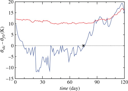
Fig. 2.  The same as in Fig. 1 but for Lake Sniardwy.

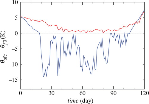
An asterisk in Fig. 1 shows the observed time of the Neusiedlersee break-up (http://www.wassernet.at, Hydrographisches Jahrbuch von Österreich 2006). The simulated break-up date is in very good agreement with observations. The lake freeze-up (middle of December according to the observations) occurs too late in the model. The delay is apparently due to a too high temperature from the routine COSMO SST analysis that was used to initialise COSMO on 1 January 2006. Then, it took a long time for the model to cool the lake water down to the freezing point. Unfortunately, no data have been found on the time of freeze-up and break-up of Lake Sniardwy in 2005–2006. Observations indicate (e.g. World Lake Database, http://wldb.ilec.or.jp) that Lake Sniardwy is typically covered by ice over several months. Apparently it was the case in 2006 which is well captured by COSMO using FLake. The temperature from the routine COSMO SST analysis indicates that Lake Sniardwy was ice-free. The same is true for numerous other lakes that are frozen in reality and in the COSMO model using FLake but remain ice-free according to the COSMO SST analysis.

Pre-operational testing of FLake within COSMO indicated a neutral to slightly positive effect of FLake on the overall performance of COSMO. Some verification scores were improved, e.g. bias and root-mean-square error (r.m.s.e.) of the two-metre temperature in regions with many lakes (Northern Europe) were reduced. As discussed above, the introduction of FLake removed a strong overestimation of the lake surface temperature during winter. Since 15 December 2010, the lake parameterisation scheme FLake is used operationally within the COSMO-EU (Europe) configuration of the COSMO model (horizontal mesh size of about 7 km). The operational results are monitored.

3.2. Sea-ice scheme in COSMO

The sea-ice scheme is used at DWD within COSMO-EU. Prior to the implementation of the scheme into the COSMO model, the surface temperature of the grid boxes indicated as ice-covered by the data assimilation scheme (fractional ice cover in excess of 0.5) was determined within the framework of the COSMO SST analysis on the basis of the ice surface temperature from GME. The procedure includes the interpolation of GME data onto the COSMO-model grid and some rather ad hoc adjustment of the ice surface temperature (see Schulz, 2011, for details). That procedure was performed once a day at 00 UTC (Coordinated Universal Time). The ice surface temperature was then kept constant over the entire forecast period (78 h for COSMO-EU). If the sea-ice model is used, the ice surface temperature varies during the forecast in response to the atmospheric forcing.

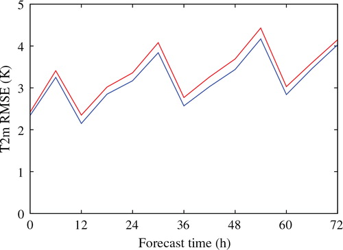
The implementation of the sea-ice scheme favourably affected the quality of the COSMO-EU forecast. Results from numerical experiments showed an improved prediction of some meteorological fields, e.g. of temperature and humidity in the lower troposphere. By way of illustration, bias and r.m.s.e. of the two-metre temperature for a part of the COSMO-EU domain in February 2010 are shown in Figs. 3 and 4. The ‘verification domain’ covers most of the Baltic Sea and the surrounding land (see Fig. 6 in Schulz, 2011). The curves are computed using observational data from the land-based meteorological stations in the neighbourhood of the Baltic Sea. As seen from the figures, the two-metre temperature forecast is significantly improved. As the COSMO-EU domain is large and has only very few ice-covered grid boxes as compared to the total number of grid boxes in the model domain, the scores averaged over the entire COSMO-EU domain are little affected by the sea-ice scheme. The local effect is substantial, however.

Fig. 3.  Bias of the two-metre temperature (T2m) vs. forecas time for the period from 3 to 28 February 2010. Lines show the COSMO-EU forecasts initialised at 00 UTC: blue line – with the sea-ice scheme, and red line – without the sea-ice scheme. Observational data used for verification are from the land meteorological stations in the neighbourhood of the Baltic Sea (see text for further explanations).

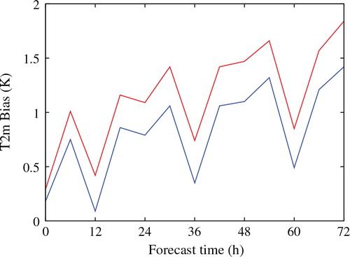
Fig. 4.  The same as in Fig. 3 but for the two-metre temperature r.m.s.e.

The sea-ice scheme is operational at DWD within COSMO-EU since 2 February 2011. The results are monitored. A quantitative assessment of the operational scheme performance will be made later, as the operational verification results over a sufficiently long period become available.

3.3. Sea-ice scheme in GME

The sea-ice parameterisation scheme described in the present paper (the ‘new scheme’) was implemented into GME and tested through numerical experiments including data assimilation. The GME output was compared with available empirical data and with the output from GME using an old ice scheme. As the lake parameterisation scheme is not implemented into GME, the sea-ice scheme applies to the ocean, seas and the inland water bodies. The ‘old scheme’ is actually a parameterisation rule that was used operationally in GME until April 2004. It simply sets the ice surface temperature to a climatologically mean value, which originates from the European Centre for Medium-Range Weather Forecasts (ECMWF) climatology (see Brankovic and Van Maanem, 1985), and keeps it constant over the entire forecast period once the ice fraction in excess of 0.5 is detected during the initialisation. That is, the atmosphere–ice interaction was basically lacking in GME with the old ice scheme.

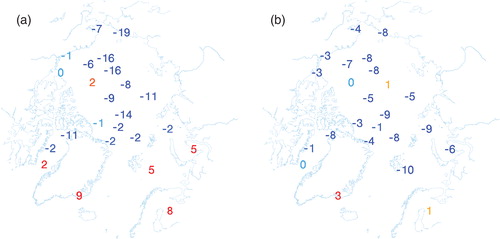
Figure 5 exemplifies the two-metre temperature in the Arctic as computed by GME with the new and the old ice schemes versus observations. The simulation with the new ice scheme shows a better agreement with data. The results with the new scheme reveal a somewhat lower bias of −4.5 K versus −5.9 K for the simulation with the old scheme and a lower r.m.s.e., 3.6 K versus 7.2 K, respectively. In spite of scarcity and possible uncertainties of available observational data, this counts in favour of the new ice scheme. Still the surface layer in GME is somewhat too cold. Pre-operational testing showed a marginal impact of the new ice scheme on the quality of the global forecast (although local effects may be significant). By and large this result was taken as satisfactory, considering that the new scheme introduced an extra degree of freedom into GME. On 31 March 2004, the new GME ice scheme became operational. The scheme performance has been monitored.

Fig. 5.  The two-metre temperature bias in the Arctic at 12 UTC 1 January 2004: left panel – GME analysis using the old ice scheme, right panel – GME analysis using the ice scheme described in the present paper. Numbers show computed minus observed two-metre temperature difference (K).

In Figs. 6 7 8 , the operational GME results for the period from 30 January 2009 to 19 January 2011 are compared with the results from the ECMWF Integrated Forecast System (IFS). The ECMWF ice scheme (see the IFS documentation at http://www.ecmwf.int) predicts the ice surface temperature by solving a four-layer finite-difference analogue of the one-dimensional heat transfer equation for the ice slab of a fixed depth of 1.5 m. In the ECMWF ice scheme, the grid-box mean surface temperature θ _g is computed with due regard for the open water fraction as the weighted-mean of the surface temperatures of the ice-covered and the ice-free parts of the grid box. In GME, θ _g is simply equal to the ice surface temperature if the ice fraction is greater than 0.5.

Fig. 6.  The grid-box mean surface temperature θ _g in the Arctic over the period from 30 January 2009 to 19 January 2011. Curves show the 24 h forecasts initialised at 00 UTC: blue curve – GME, and red curve – ECMWF. The curves are computed by means of averaging over all sea-ice points north of 65 N latitude using the GME ice-water mask.

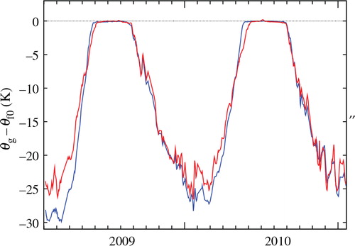
Fig. 7.  The net surface long-wave radiation flux Q _lw (positive downward) in the Arctic over the period from 30 January 2009 to 19 January 2011. Curves show values averaged over the first 24 hours of the forecast initialised at 00 UTC: blue curve – GME, and red curve – ECMWF. The curves are computed by means of averaging over all sea-ice points north of 65 N latitude using the GME ice-water mask.

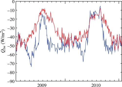
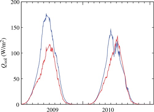
Fig. 8.  The same as in Fig. 7 but for the net surface flux of solar radiation Q _sol (positive downward).

Figure 6 shows the grid-box mean surface temperature in the Arctic from the GME and the ECMWF IFS 24 h forecasts initialised at 00 UTC. The GME surface temperature is noticeably lower than the ECMWF IFS surface temperature during February–March 2009 and January–March 2010. The neglect of the open water contribution to the grid-box mean temperature may adversely affect the GME results. This can explain a too low surface temperature in the marginal ice zone. However, this may not be of primary importance in the Central Arctic. In the middle of winter, the ice fraction there is likely to be close to 1, so that the weighted-mean surface temperature is close to the ice surface temperature. One more likely reason is that GME (at least in its configurations up to the summer 2010) tends to underestimate cloud cover in the polar regions.

Consider the situation during polar night, when there is no solar radiation input to the ice surface. Then, the ice surface temperature tends to bring the system to a quasi-equilibrium state where the upward heat flux through the ice is balanced by the heat flux at the air–ice interface, i.e. the sum of the sensible and latent heat fluxes and the long-wave radiation fluxes. In the case of constant (in time) surface heat flux, this quasi-equilibrium state is characterised by a linear temperature profile within the ice slab whose thickness increases at an ever decreasing rate. It is important to note that both a bulk scheme and a finite-difference scheme of the ice slab would reproduce this quasi-equilibrium state in the same way. The linear profile is explicitly assumed in the bulk scheme, and it appears as a steady-state solution to the heat transfer equation in the finite-difference scheme. In the case of time-dependent atmospheric forcing, the two schemes would still behave in a similar manner provided the time scale of changes in forcing is comparable to the time scale of changes in the ice temperature. This is likely the case during polar night.

For the purpose of illustration, we neglect the sensible and latent heat fluxes (these are typically small in the strongly stable boundary layer over a cold ice surface) and consider the radiation-conduction equilibrium. Then, the ice surface heat budget is6

where F _a is the downward (negative) long-wave radiation flux from the atmosphere, ɛ is the surface emissivity and σ=5.67·10⁻⁸Jm⁻²s⁻¹K⁻⁴ is the Stefan-Boltzmann constant. Using a power-series expansion of in and keeping only the leading-order term, we approximate . Then, Eq. (6) is simplified to give an explicit formula for θ _i . It reads7

The ice surface temperature depends on the downward long-wave radiation flux from the atmosphere that in turn strongly depends on the cloudiness and the radiation properties, of clouds. With the estimates of ɛ=0.99, J m⁻¹ s⁻¹ K⁻¹, θ _f =271.45 K, and H _i =1.5 m, Eq. (7) suggests that a change of 20 W m⁻² in the downward long-wave radiation flux (from −190 W m⁻² to −210 W m⁻²) results in a change in the ice surface temperature of more than 3 K.

Figure 7 compares the surface long-wave radiation budget Q _lw in GME and in ECMWF IFS. During February–March 2009 and January–March 2010, the net surface energy loss due to long-wave radiation is slightly larger in GME in spite of the fact that the ice surface in GME is colder than in ECMWF IFS by 3-5 K (Fig. 6). This suggests that the downward long-wave radiation flux from the atmosphere is lower in GME than in ECMWF IFS. As already noted, the most probable cause of discrepancy is an underestimation of cloudiness in GME.

That the GME clouds are responsible is corroborated by Fig. 8, showing the flux of solar radiation Q _sol that penetrates into the ice interior, i.e. the surface solar-radiation budget. During summer 2009, the difference in Q _sol between GME and ECMWF IFS is large. It exceeds 50 W m⁻² in the middle of summer. The difference is so substantial that it cannot be explained by a difference in the ice albedo with respect to solar radiation between GME and ECMWF IFS only. The incident solar radiation flux at the surface must also differ between the two NWP models. As this flux strongly depends on the cloudiness, too large GME values indicate that the cloudiness in polar regions is underestimated. During summer, this does not affect the ice surface temperature as it remains close to the freezing point. As seen from Fig. 6, this is indeed the case in both GME and ECMWF IFS. However, the surface solar-radiation budget may have a pronounced effect on the rate of ice melting.

The above results suggest that the ice scheme performance within an NWP model is not overly sensitive to details of the ice model itself, more specifically, to details of the treatment of heat transfer through the ice layer (the neglect of open water fraction within a grid box may, of course, play a detrimental role). This justifies the use of a simplified bulk approach to model the ice thermodynamics in NWP. The quality of the forecast of the ice characteristics is sensitive to cloud cover as it controls the radiation input to the ice surface. During 2010, numerous modifications in the physical parameterisation package and in the data assimilation package of GME were implemented. Some of those modifications, e.g. changes in the microphysics scheme, lead to an increased cloud cover in GME. Note that the difference in θ _g between GME and ECMWF IFS in December 2010 and January 2011 (Fig. 6) is considerably reduced as compared to the previous two winters. The difference in Q _sol (Fig. 8) during summer 2010 is also reduced as compared to the summer 2009.

4. Effect of snow above the ice

In this section, the effect of snow layer above the ice is discussed using results of single-column simulations of snow and ice in Lake Pääjärvi performed with the lake model FLake. Lake Pääjärvi (61.06 N, 25.13 E) is a fresh-water lake located in Finland. The lake has an area of 13.5 km², a maximum depth of 87 m and a mean depth of 15 m. It is frozen for a considerable part of the year (Leppäranta et al., 2006).

FLake was initialised on 1 May 1999 with the observed values of the water temperature (the water column was vertically homogeneous) and was run until 1 June 2000, using the lake depth of 15 m (the mean depth of Lake Pääjärvi) and the measured values of surface-layer meteorological quantities to compute surface fluxes of heat and momentum. Unfortunately, no measurements of meteorological quantities were taken over the lake surface. Only data from meteorological measurements at the shore-based station are available. The downward atmospheric flux of long-wave radiation was not measured. This flux is estimated using an empirical recipe and the observed values of the air temperature and humidity in the surface-layer and of cloud cover. The rate of snow accumulation is estimated on the basis of the observed precipitation rate, using the near-surface air temperature of 274.15 K to discriminate between the snowfall and the rainfall (the effect of rain water is ignored).

The snow surface albedo with respect to solar radiation is computed from Eq. (5), where the minimum and maximum values of albedo are 0.60 and 0.75, respectively. The following formulations are used to compute the snow density ρ _s and the snow heat conductivity κ_s:8 9

Here,  Kg m⁻³ is the density of fresh water, and ρ_min=1·10² Kg m⁻³, ρ_max=4·10² Kg m⁻³,  Kg m⁻⁴,  J m⁻¹ s⁻¹ K⁻¹,  J m⁻¹ s⁻¹ K⁻¹, and J m⁻² s⁻¹ K⁻¹ are disposable parameters. Note that the above estimates of and differ from the default FLake values of  Kg m⁻⁴ and  J m⁻¹ s⁻¹ K⁻¹ (see http://lakemodel.net). The default values are found to yield a too low snow density and a too high snow temperature conductivity (E. Kourzeneva, 2011, personal communication). Except for the snow surface albedo, snow density and snow heat conductivity, the default estimates of the FLake disposable parameters are used in the simulations (see Mironov, 2008; Mironov et al., 2010; further information is available at http://lakemodel.net).

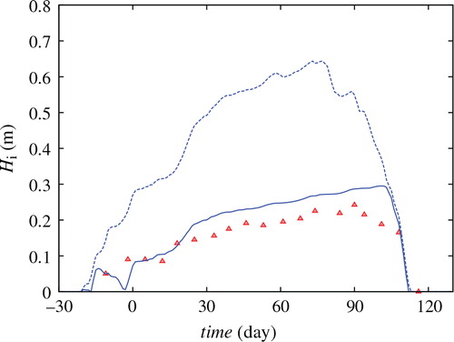
In Fig. 9, results of simulations of the ice thickness with and without a snow layer above the ice are compared with observational data. As seen from the figure, the snow insulation prevents an excessive ice growth and results in the simulated ice thickness that is in good agreement with observations. In the simulation without a snow layer above the ice, where the effect of snow is accounted for implicitly, the ice thickness is overestimated over most of the ice-cover period. However, the break-up date is very little affected as the ice melting sets in earlier if snow insulation effect is not taken into account. These results corroborate earlier findings of Dutra et al. (2010) and Kourzeneva et al. (E. Kourzeneva, 2011, personal communication).

Fig. 9.  Ice thickness in Lake Pääjärvi during winter 1999–2000, where day=0 corresponds to 1 January 2000. Blue curves show results of simulations with FLake: solid curve – with a snow layer above the ice, and dashed curve – no snow above the ice. Red symbols show observational data.

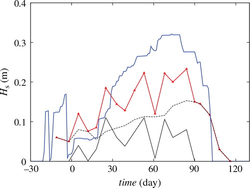
Figure 10 compares the simulated snow thickness with observational data. In the observations, both the snow thickness (snow ‘per se’) and the snow ice thickness are given. The formation of snow ice is not considered in the ice-snow module of FLake, however. Then, the layers of snow and snow ice are put together, and the observed total thickness of the two layers (red curve with symbols in Fig. 10) is compared with the simulated snow layer thickness (blue curve). A fair agreement between empirical data and simulation results is found. The agreement is not as good as for the ice thickness. This is not surprising, considering possible large uncertainties in the atmospheric forcing. Yet another source of uncertainties are the simplified, perhaps oversimplified, parameterisations of the snow density and the snow heat conductivity (in the formulations used, ρ _s and are functions of the snow thickness H _i only). Results from test runs (not shown) revealed large sensitivity to the values of disposable parameters in Eqs. (8) and (9). A satisfactory performance of the scheme in the Lake Pääjärvi test case (Figs. 9 and 10) does not guarantee a similar performance in the other cases unless the disposable parameters in the formulations of ρ _s and are adjusted (‘re-tuned’). This is possible in single-column off-line mode, although re-tuning should be considered as a bad practice and must be avoided whenever possible as it greatly reduces the predictive capacity of a physical model (Randall and Wielicki, 1997). Re-tuning is clearly not possible within NWP and climate models, whose numerical domains are large and very different situations are encountered during a model run. More physically plausible and more flexible parameterisations of ρ _s and are required.

Fig. 10.  Snow thickness in Lake Pääjärvi during winter 1999–2000, where day=0 corresponds to 1 January 2000. Blue curve is computed with FLake. Black solid and dashes curves show observed values of the snow thickness and the snow ice thickness, respectively. Red curve with symbols shows the total thickness of the two layers.

The lake surface temperature as simulated by FLake with and without a snow layer above the ice is shown in Fig. 11. During most of the period of ice cover, the surface temperature in the simulation without snow (i.e. the ice surface temperature) exceeds the surface temperature in the simulation with snow (i.e. the temperature of either snow surface or ice surface depending on whether snow above the ice is present). The ice break-up date is captured well in both simulations, and the evolution of the water surface temperature following the ice break-up is in good agreement with observational data. Unfortunately, no data are available to quantitatively assess the performance of the scheme with respect to the surface temperature of ice and snow. Such an assessment should be performed as reliable empirical data become available.

Fig. 11.  Surface temperature of Lake Pääjärvi during winter 1999–2000, where day=0 corresponds to 1 January 2000. The lake surface temperature is equal to the surface temperature of snow, ice or water depending on which surface is exposed to the atmosphere (snow, ice or open water). Blue solid and dashed curves show results of simulations with and without a snow layer above the ice, respectively. Red curve shows observed water surface temperature.

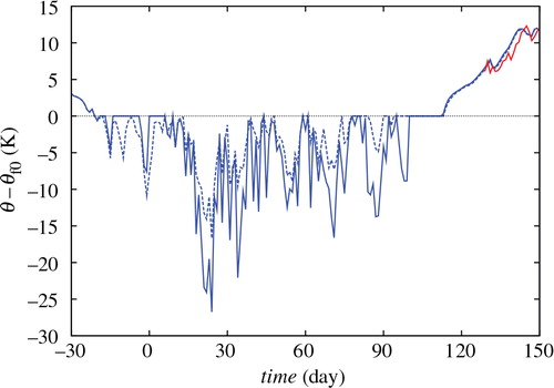
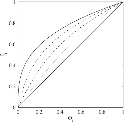
Fig. 12.  The approximation of the temperature-profile shape function with the third-order polynomial whose coefficients satisfy Eq. (B.1). The curves are computed with and (from right to left) , , , , and .

5. Conclusions

A bulk thermodynamic sea-ice parameterisation scheme is developed and implemented into the global NWP model GME and the limited-area NWP model COSMO of DWD. A distinguishing feature of the proposed scheme is the treatment of the heat transfer through the ice. Most currently used ice schemes carry the heat transfer equation that is solved on a finite difference grid where the number of grid points and the grid spacing differ with the application. The proposed scheme uses the integral, or bulk, approach. It is based on a parametric representation (assumed shape) of the evolving temperature profile within the ice and on the integral heat budget of the ice slab. The proposed ice scheme solves two ordinary differential equations for the two time-dependent quantities, viz., the ice surface temperature and the ice thickness. As regards the horizontal distribution of the sea ice cover (i.e. the existence of ice within a given GME/COSMO grid box), it is governed by the data assimilation scheme. The lake ice is treated similarly to the sea ice, except that freeze-up and break-up of lakes occur freely, independent of the data assimilation. The lake-ice module is an integral part of the fresh-water lake parameterisation scheme FLake that is implemented into COSMO.

Results from numerical experiments, including comprehensive pre-operational testing, and from the operational use of the sea-ice and lake-ice schemes show their satisfactory performance within GME and COSMO. The ice characteristics are not overly sensitive to the details of the treatment of heat transfer through the ice layer. This is an encouraging result as it justifies the use of simplified ice schemes in NWP. The use of an integral approach instead of a finite-difference approach allows to save computational resources without any detectable loss in accuracy of the results. The operational implementation of the sea-ice and lake-ice schemes into NWP models of DWD resulted in an improved interactive coupling of the atmosphere with the underlying surface. Verification results indicate improvements in terms of the surface temperature and some verification scores, e.g. bias and r.m.s.e. of the near-surface temperature and humidity. The sea-ice scheme and the lake-ice scheme (as part of the lake parameterisation scheme FLake) are currently used within the COSMO-EU (Europe) configuration of the COSMO model operational at DWD. The operational implementation of the schemes into the high-resolution (horizontal mesh size of ca. 2.8 km) COSMO-model configuration COSMO-DE (Germany) is underway at DWD. Both the sea-ice scheme and FLake will be implemented into the new global model ICON.

As the results from numerical experiments suggest, the ice characteristics are very sensitive to cloud cover as it controls the radiation energy budget at the ice surface. During winter, when solar radiation input to the ice surface is close to zero, the downward long-wave radiation flux from the atmosphere is of decisive importance for the ice surface temperature. During summer, the surface radiation budget is also sensitive to the grid-box mean ice surface albedo with respect to solar radiation. Changes in the ice albedo would not substantially affect the ice surface temperature as it remains close to the freezing point, but they may have a pronounced effect on the rate of ice melting. In the present operational configuration of GME and COSMO, an empirical formulation is used, where the ice albedo depends on the ice surface temperature. That formulation is meant to implicitly account, in a rather crude way, for the seasonal albedo changes.

In view of the crucial importance of the surface radiation budget, future efforts should go into the development of a refined formulation of the grid-box mean surface albedo. To this end, an improved parameterisation of the albedo of ice itself and the consideration of the fractional ice cover are essential. NWP models may also benefit from an explicit treatment of snow above the sea and lake ice. In Appendix A, the way to account for the snow layer above the ice using a bulk parameterisation framework is outlined. As the results from numerical experiments discussed in Section 4 suggest, the bulk snow modelling framework is of considerable promise. However, the necessary empirical information is lacking at present. In particular, improved formulations for the snow density and the snow temperature conductivity are required to account for the dependence of these quantities on the snow depth and temperature, on the snow age, and, perhaps, on other parameters. Until such formulations are developed and considering numerous other uncertainties of current NWP models (most notably in terms of cloudiness), simplified bulk sea and lake ice parameterisation schemes with an implicit treatment of snow seem to be sufficient for NWP.

6. Acknowledgements

Thanks are due to Ulrich Damrath, Jochen Förstner, Sergej Golosov, Thomas Hanisch, Erdmann Heise, Georgiy Kirillin, Ekaterina Kourzeneva, Aurelia Müller, Van-Tan Nguyen, Ulrich Schättler, Natalia Schneider, Christoph Schraff, Arkady Terzhevik and Miklós Vörös for numerous discussions and helpful suggestions. The authors are particularly grateful to Ulrich Damrath, Jochen Förstner, Thomas Hanisch and Ulrich Schättler for their invaluable help in implementing and testing the new ice parameterisation schemes in GME and COSMO. Comments of the anonymous reviewers helped to considerably improve the manuscript. Empirical data from Lake Pääjärvi are made available through the collaboration with the Division of Geophysics of the University of Helsinki that is supported by the Academy of Finland (project ‘Ice Cover in Lakes and Coastal Seas’) and by the Vilho, Yrjö and Kalle Väisälä Foundation of the Academy of Sciences and Letters, Finland (project ‘Modelling of Boreal Lakes’). The ECMWF forecast products used for comparison are taken from the ECMWF MARS archive. The work was partially supported by the EU Commissions through the projects INTAS-01-2132 and INTAS-05-1000007-431, and by the Nordic Research Board through the Nordic Networks on Fine-Scale Atmospheric Modelling (NetFAM) and Towards Multi-Scale Modelling of the Atmospheric Environment (MUSCATEN).

Notes

¹The terms ‘parameterisation scheme’ and ‘model’ can be used interchangeably. The term ‘parameterisation scheme’ is used in the NWP and climate modelling community to differentiate a component (module) of a modelling system from its host that is referred to as an NWP (climate) model.

²Notice a close analogy between the concept of self-similarity of the thermocline and the mixed-layer concept that has been successfully used in geophysical fluid dynamics over several decades. Indeed, using the mixed-layer temperature and its depth as appropriate scales, the mixed-layer concept states that the dimensionless temperature profile can be expressed through a universal function of dimensionless depth, where that universal function is simply a constant equal to one, that is , where . A function that describes the temperature profile in the thermocline is not merely a constant but a more sophisticated function of dimensionless depth.

³Equation (1) is merely Eq. (A.9) with . Equation (2) is obtained from Eq. (A.5) with H _s =0 and I(0)=0 by replacing ρ _s  c _s  θ _s on the left-hand side of Eq. (A.5) with ρ _i  c _i  θ _i and using Eq. (1). Equation (3) is obtained by setting θ _s =θ _i , ρ _s =ρ _i , H _s =0, dH _s /dt=0 and in Eq. (A.10) and adding the result to Eq. (A.11) with I(0)=0. The resulting system of equations, namely Eqs. (1)–(4), can be arrived at by performing derivations in Appendix A with H _s ≡0 from the outset.

Appendix AFormulation of the ice parameterisation scheme

A.1. Governing equations

In the sea-ice scheme presented below, provision is made to account for the heat flux from water to ice, for the volumetric character of the solar radiation heating, and for the snow layer above the ice. Recall that a simplified version of the scheme is currently used within GME and COSMO, where these features are neglected (see Section 2).

The equations of the ice-snow scheme are derived from the heat transfer equationA.1

Here, t is time, z is the vertical co-ordinate (positive upward) with the origin at the ice-water interface, ρ and c are the density of the medium in question (snow or ice) and its specific heat, respectively, θ is the temperature, I is the solar radiation flux, Q is the vertical heat flux (the long-wave radiation fluxes are assumed to enter through the boundary condition at the lower boundary of the atmosphere), M is the mass of snow or ice per unit area, and L _f is the latent heat of fusion. The last term on the right-hand side of Eq. (A.1) is the source term that describes the rate of heat release/consumption due to accretion/melting of snow and ice. The function f _M (z) satisfies the normalization conditionsA.2

where H _i is the ice thickness, and H _s is the thickness of snow overlaying the ice.

The ice-snow scheme presented below includes a number of thermodynamic parameters. These can be considered constant except for the snow density and the snow heat conductivity that depend, among other things, on the snow thickness and the snow age and are, therefore, time-dependent.

A.2. Parameterisation of the temperature profile

We adopt the following parametric representation of the evolving temperature profile within ice and snow:A.3

Here, θ _f is the freezing point at the underside of the ice, θ _i is the temperature at the snow-ice interface, and θ _s is the temperature at the air-snow interface. The freezing point θ _f is a decreasing function of salinity that is equal to the fresh-water freezing point θ _f0 when the salinity is zero. Dimensionless universal functions and of dimensionless vertical coordinates and , respectively, satisfy the boundary conditions Φ _i (0)=0, Φ _i (1)=1, Φ _s (0)=0 and Φ _s (1)=1. In what follows, the arguments of functions dependent on time and vertical coordinate are not indicated, unless it is indispensable.

According to Eq. (A.3), the heat fluxes through ice, Q _i , and through snow, Q _s , due to molecular heat conduction are given byA.4

where and are the heat conductivities of ice and snow, respectively.

A.3. Heat budget

The parameterisation of the temperature profile (A.3) should satisfy the heat transfer equation (A.1). Consider first the regime where no melting at the snow upper surface (ice upper surface, when snow is absent) takes place. In this regime, the heat flux Q is continuous at z=H _i +H _s , whereas it may undergo a zero-order jump at the ice-water interface where the ice ablation/accretion takes place. Then, the normalization function f _M is equal to zero throughout the snow and ice layers except at the ice-water interface where f _M = δ(0), δ(z) being the Dirac delta function. Integrating Eq. (A.1) over z from just above the ice-water interface z=+0 to the air-snow interface z=H _i +H _s with due regard for the parameterisation of the temperature profile (A.3), we obtain the equation of the heat budget of the snow and ice cover,A.5

Here, ρ _i and ρ _s are the densities of ice and of snow, respectively, c _i and c _s are specific heats of these media, I _a is the solar radiation flux at the air-snow or, if snow is absent, at the air-ice interface, and Q _a is the heat flux in the air layer adjacent to the snow (ice) surface. Hereafter, a prime denotes derivatives of the shape functions Φ _i and Φ _s with respect to the dimensionless vertical coordinates and , respectively. The radiation heat flux I _a that penetrates into the interior of the snow and ice cover is the surface value of the incident solar radiation flux from the atmosphere multiplied by 1−α, α being the surface albedo of snow or ice with respect to solar radiation. The heat flux Q _a is a sum of the sensible and latent heat fluxes and the long-wave radiation fluxes at the air-snow (air-ice) interface. It is a rather sophisticated function of the surface air layer parameters, of cloudiness and of the temperature at the air-snow (air-ice) interface. The dimensionless parameters and , the so-called ‘shape factors’, are given byA.6

The heat flux due to molecular heat conduction is assumed to be continuous at the snow-ice interface, that isA.7

It must be emphasized that in the framework of the bulk approach the exact knowledge of the shape functions Φ _i and Φ _s is not required. It is not Φ _i and Φ _s per se, but the shape factors and and the dimensionless gradients , and that enter the resulting model equations.

Equations (A.5) and (A.7) serve to determine the temperatures at the air-snow and at the snow-ice interfaces, when no melting at the snow upper surface (ice upper surface, when snow is absent) takes place. During the snow (ice) melting from above, the surface temperature remains equal to the freezing point.

A.4. Snow and ice thickness

The accumulation of snow is not computed within the ice-snow scheme. The rate of snow accumulation is assumed to be a known time-dependent quantity that is provided by the host atmospheric model or is known from observations. Then, the evolution of the snow thickness during the snow accumulation and no melting is computed fromA.8

where M _s =ρ _s H _s is the snow mass per unit area, and is the (given) rate of snow accumulation.

Considering the sea ice, the effect of internal brine pockets (e.g. Semtner, 1976) is neglected. Brine rejection leads to desalinization of the sea ice and hence to the increase of its freezing point. This effect is accounted for parametrically, in a rather approximate way, by setting the freezing point at the upper surface of the ice to the fresh-water freezing point θ _f0. When the temperature θ _i at the upper surface of the ice (θ _i is equal to θ _s if snow is absent) is below the freezing point θ _f , the heat conduction through the ice causes the ice growth. This growth is accompanied by a release of heat at the lower surface of the ice that occurs at a rate , where M _i =ρ _i H _i is the ice mass per unit area. Integrating Eq. (A.1) over z from z=−0 to z=+0, where the heat source term due to the ice accretion is , we obtain the equation for the ice thickness. It readsA.9

where Q _w is the heat flux from water to ice. When the heat flux from water to ice exceeds the heat flux within the ice, ice ablation takes place.

As the atmosphere heats the snow surface, the surface temperature increases and snow melting eventually sets in. Since snow consists of fresh water, melting starts when the surface temperature reaches the fresh-water freezing point θ _f0. The snow melting is accompanied by a consumption of heat in the snow layer that occurs at a rate . Notice that the exact form of the normalization function f _M is not required by virtue of the normalization condition given by the first member of Eq. (A.2). Integrating Eq.  (A.1) over z from z=H _i to z=H _i +H _s +0 with due regard for the heat loss due to snow melting, then adding the (given) rate of snow accumulation, we obtainA.10

where and .

The ice melting is accompanied by a consumption of heat at a rate . Again, the exact form of the function f _M is not required by virtue of the normalization condition given by the second member of Eq. (A.2). Integrating Eq.  (A.1) over z from z=−0 to z=H _i , we obtainA.11 where .

During the snow melting, the surface temperature remains equal to the fresh-water freezing point, θ _s =θ _f0, and the temperature θ _i is computed from Eq. (A.7).

Notice finally that ice melting may occur at the lower surface of the ice, even though there is no heating from the water below the ice. Brine rejection from the sea ice leads to its desalinization. This results in a salinity gradient across the ice and hence in a difference in the freezing point between the upper and lower surfaces of the ice. Close to the upper surface, the ice is almost free of salt so that the freezing point there is close to the fresh-water freezing point θ _f0. At the lower surface, the freezing point is that of salt water which is lower than θ _f0. Taking the freezing point at the upper surface of the ice to be equal to the fresh-water freezing point, ice melting may occur at its lower surface due to heat conduction caused by the temperature difference across the ice. The evolution of the ice thickness in this regime is governed by Eq. (A.9). The evolution of θ _i and θ _s is governed by Eqs. (A.5) and (A.7).

Appendix BThe temperature-profile shape function

Although a linear profile is a good approximation for thin ice, it is likely to result in a too thick ice in cold regions, where the ice growth takes place over most of the year, and in a too high thermal inertia of thick ice. A slightly more sophisticated approximation is developed by assuming that the ice thickness is limited by a certain maximum value H _imax and that the rate of ice grows approaches zero as H _i approaches H _imax. We proposeB.1

where Φ_* is a dimensionless constant. The physical meaning of the above expressions can be elucidated as follows. The first member of Eq. (B.1) ensures that the ice growth is quenched as the ice thickness approaches its maximum value. The second member of Eq. (B.1) suggests that the shape factor decreases with increasing ice thickness. A smaller means a smaller relative thermal inertia of the ice layer of thickness H _i [the absolute thermal inertia is measured by the term that multiplies on the left-hand side of Eq. (2)]. This is plausible as it is mostly the upper part of thick ice, not the entire ice layer, that effectively responds to atmospheric forcing. The ice scheme has only two tuning parameters. A reasonable estimate of the maximum ice thickness is H _imax =3 m. The allowable values of lie in the range between −1 and 5. yields an unphysical negative value of as the ice thickness approaches H _imax. gives that increases with increasing H _i . There is no formal proof that this may not occur, but it is very unlikely. A reasonable estimate is . With this estimate is halved as H _i increases from 0 to H _imax. Notice that the linear temperature profile is recovered as , i.e. when the ice is thin.

One further comment is in order regarding the expressions (B.1). These expressions may be viewed as corresponding to the third-order polynomial approximation of the temperature-profile shape function . The third-order polynomial is the simplest approximation that satisfies a minimum set of constraints. The polynomial coefficients are determined as follows. First, the boundary conditions Φ _i (0)=0 and Φ _i (1)=1 are satisfied that simply follow from the definition of Φ _i and . Second, the conditions (B.1) are satisfied, where the shape factor is defined through the first member of (A.6). The dependence of and on is chosen so that to ensure the desired behaviour of the ice growth rate and of the thermal inertia of the ice layer. This approach, that could be called ‘verifiable empiricism’, heavily relies on empirical data. However, it still incorporates much of the essential physics and offers a good compromise between physical realism and computational economy. The third-order polynomial approximation of the temperature-profile shape function is illustrated in Fig. 12. As seen from the figure, the temperature profile is almost linear when the ice is thin, , and is given by the left solid curve as the ice thickness H _i approaches its maximum value H _imax.

References

- Arsenyev S. A. Felzenbaum A. I. Integral model of the active ocean layer. Izv. Akad. Nauk SSSR. Fizika Atmosfery i Okeana. 1977; 13: 1034–1043.
- Baldauf, M, Seifert, A, Förstner, J, Majewski, D, Raschendorfer, M and Reinhardt, T. 2011. Operational convective-scale numerical weather prediction with the COSMO model: description and sensitivities. Mon. Weather Rev. 139, 3887–3905. DOI: 10.1175/MWR-D-10-05013.1.
- Bitz C. M. Libscomb W. H. An energy-conserving thermodynamic model of sea ice. J. Geophys. Res. 1999; 104: 15669–15677.
- Brankovic, C and Van Maanem, J. 1985. The ECMWF climate system. Research Department Technical Memorandum 109. European Centre for Medium-Range Weather Forecasts, Reading.
- Cheng B. Launiainen J. Vihma T. Modelling of superimposed ice formation and sub-surface melting in the Baltic Sea. Geophysica. 2003; 39: 31–50.
- Deardorff J. W. Prediction of convective mixed-layer entrainment for realistic capping inversion structure. J. Atmos. Sci. 1979; 36: 424–436.
- Dutra, E, Stepanenko, V. M, Balsamo, G, Viterbo, P, Miranda, P. M. A, Mironov, D and Schär, C. 2010. An offline study of the impact of lakes on the performance of the ECMWF surface scheme. Boreal Env. Res. 15, 100–112.
- Ebert E. E. Curry J. A. An intermediate one-dimensional thermodynamic sea ice model for investigating ice-atmosphere interactions. J. Geophys. Res. 1993; 98: 10085–10109.
- Fedorovich E. E. Mironov D. V. A model for a shear-free convective boundary layer with parameterized capping inversion structure. J. Atmos. Sci. 1995; 52: 83–95.
- Filyushkin B. N. Miropolsky Y. Z. Seasonal variability of the upper thermocline and self-similarity of temperature profiles. Okeanologia. 1981; 21: 416–424.
- Golosov, S and Kirillin, G. 2010. A parameterized model of heat storage by lake sediments. Env. Modell. Softw. 25, 793–801. DOI: 10.1016/j.envsoft.2010.01.002.
- Kamenkovich V. M. Kharkov B. V. On the seasonal variation of the thermal structure of the upper layer in the ocean. Okeanologia. 1975; 15: 978–987.
- Kirillin G. Modeling the impact of global warming on water temperature and seasonal mixing regimes in small temperate lakes. Boreal Env. Res. 2010; 15: 279–293.
- Kirillin, G, Hochschild, J, Mironov, D, Terzhevik, A, Golosov, S and Nützmann, G. 2011. FLake-Global: Online lake model with worldwide coverage. Env. Modell. Softw. 26, 683–684. 10.3402/tellusa.v64i0.17330.
- Kitaigorodskii S. A. Miropolsky Y. Z. On the theory of the open ocean active layer. Izv. Akad. Nauk SSSR. Fizika Atmosfery i Okeana. 1970; 6: 178–188.
- Launiainen J. Cheng B. Modelling of ice thermodynamics in natural water bodies. Cold Reg. Sci. Technol. 1998; 27: 153–178.
- Leppäranta M. A review of analytical models of sea-ice growth. Atmos.-Ocean. 1993; 31: 123–138.
- Leppäranta, M, Wang, C, Wang, K, Shirasawa, K and Uusikivi, J. 2006.Investigations of wintertime physical processes in boreal lakes. In: Workshop on Water Resources of the European North of Russia: Results and Perspectives. (eds. N. N. Filatov, V. I. Kuharev and V. H. Lifshits), Northern Water Problems Institute, Karelian Research Centre, Russian Academy of Sciences: PetrozavodskKarelia, Russia, pp. 342–359.
- Majewski, D, Liermann, D, Prohl, P, Ritter, B, Buchhold, M, Hanisch, T, Paul, G, Wergen, W and Baumgardner, J. 2002. Icosahedral-hexagonal gridpoint model GME: description and high-resolution tests. Mon. Weather Rev. 130, 319–338.
- Maykut G. A. Untersteiner N. Some results from a time-dependent thermodynamic model of sea ice. J. Geophys. Res. 1971; 76: 1550–1575.
- Mellor G. L. Kantha L. An ice-ocean coupled model. J. Geophys. Res. 1989; 94: 10937–10954.
- Mironov, D, Heise, E, Kourzeneva, E, Ritter, B, Schneider, N and Terzhevik, A. 2010. Implementation of the lake parameterisation scheme FLake into the numerical weather prediction model COSMO. Boreal Env. Res. 15, 218–230.
- Mironov, D. V. 2008. Parameterisation of lakes in numerical weather prediction. Description of a lake model. COSMO Technical Report 11. Deutscher Wetterdienst: Offenbach am MainGermany. Online at http://www.cosmo-model.org.
- Mironov, D. V, Golosov, S. D, Zilitinkevich, S. S, Kreiman, K. D and Terzhevik, A. Y. 1991. Seasonal changes of temperature and mixing conditions in a lake. In: Modelling Air-Lake Interaction. Physical Background. (ed. S. S. Zilitinkevich). Springer-Verlag: Berlin, pp. 74–90.
- Mironov, D and Ritter, B. 2003. A first version of the ice model for the global NWP system GME of the German Weather Service. In: Research Activities in Atmospheric and Oceanic Modelling. (ed. J. Cote). WMO/TD, Report No. 33, pp. 4.13–4.14.
- Mironov, D and Ritter, B. 2004. Testing the new ice model for the global NWP system GME of the German Weather Service. In: Research Activities in Atmospheric and Oceanic Modelling. (ed. J. Cote). WMO/TD, Report No. 34, pp. 4.21–4.22.
- Omstedt A. A coupled one-dimensional sea ice–ocean model applied to a semi-enclosed basin. Tellus. 1990; 42A: 568–582.
- Omstedt, A. 1999. Forecasting ice on lakes, estuaries and shelf seas. In: Ice Physics and the Natural Environment. Vol. I: 56 of NATO ASI Series (eds. J. S. Wettlaufer, J. G. Dash and N. Untersteiner). Springer-Verlag: Berlin and Heidelberg, pp. 185–208.
- Perovich D. K. Grenfell T. C. Light B. Hobbs P. V. Seasonal evolution of the albedo of multiyear arctic sea ice. J. Geophys. Res. Oceans. 2002; 107: 8044–8056.
- Randall D. A. Wielicki B. A. Measurements, models, and hypotheses in the atmospheric sciences. Bull. Amer. Meteorol. Soc. 1997; 78: 399–406.
- Schulz, J.-P. 2011. Introducing a sea ice scheme in the COSMO model. COSMO Newsletter. 11. Online at http://www.cosmo-model.org.
- Semtner A. J. A model for the thermodynamic growth of sea ice in numerical investigations of climate. J. Phys. Oceanogr. 1976; 6: 379–389.
- Stefan J. Ueber die Theorie der Eisbildung, insbesondere über die Eisbildung im Polarmeere. Ann. Phys. Chem. 1891; 42: 269–286.
- Steppeler, J, Doms, G, Schättler, U, Bitzer, H. W, Gassmann, A, Damrath, U and Gregoric, G. 2003. Meso-gamma scale forecasts using the non-hydrostatic model LM. Meteorol. Atmos. Phys. 82, 75–96.
- Thomas, D. N and Dieckmann, G. S. (Eds.)2003. Sea ice. An Introduction to its Physics, Chemistry, Biology and Geology. Blackwell Science, 402 p.
- Zilitinkevich S. S. Turbulent Penetrative Convection. Avebury Technical: Aldershot, 1991; 179 p.
- Zilitinkevich, S. S, Fedorovich, E. E and Mironov, D. V. 1992. Turbulent heat transfer in stratified geophysical flows. In: Recent Advances in Heat Transfer. (eds. B. Sundén and A. Zukauskas). Elsevier Science Publisher B. V.: Amsterdam, pp. 1123–1139.