Snow and ice on Bear Lake (Alaska) – sensitivity experiments with two lake ice models

ABSTRACT

Snow and ice thermodynamics of Bear Lake (Alaska) are investigated with a simple freshwater lake model (FLake) and a more complex snow and ice thermodynamic model (HIGHTSI). A number of sensitivity experiments have been carried out to investigate the influence of snow and ice parameters and of different complexity on the results. Simulation results are compared with observations from the Alaska Lake Ice and Snow Observatory Network. Adaptations of snow thermal and optical properties in FLake can largely improve accuracy of the results. Snow-to-ice transformation is important for HIGHTSI to calculate the total ice mass balance. The seasonal maximum ice depth is simulated in FLake with a bias of −0.04 m and in HIGHTSI with no bias. Correlation coefficients between ice depth measurements and simulations are high (0.74 for FLake and 0.9 for HIGHTSI). The snow depth simulation can be improved by taking into account a variable snow density. Correlation coefficients for surface temperature are 0.72 for FLake and 0.81 for HIGHTSI. Overall, HIGHTSI gives slightly more accurate surface temperature than FLake probably due to the consideration of multiple snow and ice layers and the expensive iteration calculation procedure.

• snow on lake ice
• thermodynamic ice model
• heat conductivity of snow
• albedo
• snow to ice transformation

1. Introduction

In the boreal countries, a realistic representation of freezing and melting of lakes and snow on lake ice is important for numerical weather prediction (NWP) and regional climate model applications. Due to changing climate conditions, especially at higher latitudes, the lake ice season can be strongly influenced, which in turn results in a feedback on the regional climate (Brown and Duguay, 2010). It is important to couple lake ice models to climate and NWP models to simulate the two-way feedback between lakes and regional weather/climate (MacKay et al., 2009). In such a coupled model set-up, it turns out that lakes can have a net warming effect leading to a convective precipitation increase of 20–40% in late summer (Samuelsson et al., 2010). With increasing computing power, higher resolutions in limited area models become feasible. Lakes and their impact on the local weather and climate can be resolved in model grids.

Sufficient data about the lake surface state are rarely available for data assimilation in NWP or for evaluation of lake models. Detailed observations of lake ice and snow depth and temperature are sparse and mostly restricted to measurement campaigns. Therefore, a precise simulation of snow and ice cover is important but challenging.

Modelling lake ice and snow has been carried out in several studies. Heron and Woo (1994) investigated the decay of lake ice with a lake ice energy-balance model. Vavrus et al. (1996) compare simulated freezing and melting times with climatologically observed data using a simple lake model. Duguay et al. (2003) and Jeffries et al. (2005) use the Canadian Lake Ice Model CLIMo to simulate lake ice over Alaskan ponds and compare freezing and melting times as well as ice depth to observed data. Mironov et al. (2010) have implemented freshwater lake model (FLake) into the NWP model COSMO. They note that a quantitative evaluation of snow and ice in the model is challenging. Eerola et al. (2010) have reported implementation of FLake as a parameterisation scheme into the NWP model HIgh Resolution Limited Area Model (HIRLAM). They have found out that the ice cover can have an important local impact on the atmospheric surface boundary layer.

Evolution of the snow layer may add further complication to the lake ice processes. For example, the change of snow depth during the melt season is strongly dependent on the surface albedo. In addition to its insulation effect, snow may contribute to the total ice mass via snow-ice and superimposed ice formation (Cheng et al., 2003). This process has largely been observed in the Northern hemisphere ice-covered lakes and seas (Leppäranta, 1983; Kawamura et al., 1997; Nicolaus et al., 2003). Climate change scenarios suggest increasing precipitation in the Arctic (Christensen and Christensen, 2007). Therefore, snow may become more important for ice thermodynamics.

The aim of this study is to investigate how complex a lake ice model should be in order to realistically simulate snow and ice depth and temperature, how sensitive a lake ice model is to the definition of ice and snow properties, and which further processes might be necessary to consider in the parameterisations. Investigated parameters include albedo of fresh and melting snow and ice as well as snow density and heat conductivity. Two different lake ice models are compared: a simple lake model with two water layers, one ice and one snow layer (FLake: Mironov, 2008; Mironov et al., 2010) and a sea and lake ice model with multiple ice and snow layers (HIGHTSI: Launiainen and Cheng, 1998; Cheng et al., 2003). Both models are based on the solution of the heat conduction equations and do not consider the effects of ice dynamics.

A first step towards a lake ice model comparison is made in this study. While a lake model intercomparison project has already been initiated (Stepanenko et al., 2010), the emphasis is on lake temperature profiles rather than ice and snow processes. Our comparison is carried out for a small lake in the south-east of Alaska for which observations of snow depth, snow density, surface temperature, snow–ice interface temperature, conductive heat flow and snow water equivalent are measured in intervals between once every week and once every month (Jeffries and Morris, 2006; ALISON, 2011) – for the first time allowing a quantitative comparison of snow and ice properties between simulations and observations. Through the comparison of two models the most sensitive parameters can be figured out and improvements introduced into both models.

In Section 2 model descriptions of FLake and HIGHTSI are given, focusing on the snow parameterisations. Section 3 describes the observation data used for validation, section 4 the set-up of the experiments and section 5 their results. In Section 6 conclusions are drawn.

2. Models

2.1. FLake

FLake is a thermodynamic lake model. The water module considers the heat and kinetic energy budget of two layers, that is, upper mixed-layer and basin bottom. FLake is able to predict the vertical temperature structure and mixing conditions at various depths. The lake depth is an important input parameter for FLake since it determines the heat capacity, the temperature development, the freeze-up date and the heat flux from water to ice. The concept of self-similarity (Kitaigorodskii and Miropolsky, 1970) is used to describe the temperature-depth curve for all layers in vertical. The mixing-layer depth calculation includes convective entrainment and wind-mixing effect for unstable and stable regimes, correspondingly. Both mixing regimes are treated considering the volumetric character of solar radiation heating. In order to compute momentum, sensible and latent heat fluxes at the lake surface, a parameterisation scheme has been developed that accounts for specific features of the surface air layer over lakes (Mironov, 2008). In our configuration, the model considers four layers in vertical: two lake water layers, one ice and one snow layer. A detailed description of FLake is given by Mironov (2008).

We focus on improvement of snow description in FLake, which has not been thoroughly tested yet. Rather than implementing a more complex snow scheme on lake ice, special attention has been paid to parameterisation of snow properties, which have a major impact on snow and ice mass balance.

In the reference FLake, snow density (ρ _s) is a function of snow depth:1

where ρ _smax is the maximum snow density (400 kg m⁻³), ρ _smin is the minimum snow density (100 kg m⁻³) and h _s is the snow depth (m), c is an empirical parameter (200 kg m⁻⁴) and ρ _w is the water density (1000 kg m⁻³). Snow density can vary between 100 and 400 kg m⁻³. Snow accumulates through snowfall. With increasing snow accumulation the snow is compacting, that is, the snow density is increasing according to this parameterisation. However, snow would actually get less dense when snow is melting, which is physically unrealistic. Furthermore, increasing snow depths from 0.01 to 1 m would increase the snow density only from 100 and 125 kg m⁻³. Observations for Bear Lake show values between 130 and 470 kg m⁻³. Sturm and Liston (2003) noticed that snow density on the Alaska lakes is usually higher than that on the surrounding land. Average snow densities of 344 and 334 kg m⁻³ were obtained for spring 2000 and 2002 over 13 Alaskan lakes. These values are comparable to the average value of 320 kg m⁻³ for winter snow on Arctic sea ice (Huwald et al., 2005).

The snow heat conductivity (k _s) is calculated depending on the density and snow depth:2

where k _smax is the maximum snow heat conductivity (1.5 W (mK)⁻¹), k _smin is the minimum snow heat conductivity (0.2 W (mK)⁻¹). According to Eqs. (1) and (2), k _s varies between 0.2 and 0.36 W (mK)⁻¹. This is in line with a recent investigation by Ashton (2011) who argues that k _s varies between 0.1 and 0.4 W (mK)⁻¹, with typical values from 0.2 to 0.3 W (mK)⁻¹ for Northern American Arctic and Subarctic lakes. The spatial inhomogeneity, however, has an impact on the spatially averaged heat conductivity, especially when snow depth is less than 0.4 m (Sturm et al., 2002). We therefore define a variable called effective snow heat conductivity:3

where k _s is 0.14 W (mK)⁻¹, k _i is the heat conductivity of lake ice (2.29 W (mK)⁻¹), c is an empirical constant (5 m⁻¹). Eq. (3) gives higher heat conductivity for thinner snow. For thin snow, there is likely to be bare ice in the vicinity because of wind effect. Therefore, the effective snow heat conductivity would be a mixture of heat conductivity of snow and ice within a unit area.

The surface albedo (α _sfc) in the reference FLake is calculated by:4

where α ₁ refers to albedo for white ice (snow-ice) or dry snow equal to 0.6. α ₂ is albedo for blue ice (congelation ice) or melting snow which was set to 0.1. T ₀ is the freezing temperature (273.15 K), T _sfc is the surface temperature. Eq. (4) suggests the same albedo for both snow and ice. Furthermore α _sfc approaches 0.1 when T _sfc is close to T ₀ .

The albedo values given by eq. (4) differ quite a lot from in situ measurements and may not be adequate to study snow and ice mass balance. Even observed albedo shows large variations between different research sites. For example, albedo values of 0.43 and 0.21 for white ice (snow-ice) and melting ice, respectively, were observed on the Great Lakes (Bolsenga, 1977). The albedo of melting blue ice varies from 0.2 to 0.4 (Prowse and Marsh, 1989) and from 0.4 to 0.55 (Heron and Woo, 1994) depending on ice crystal orientation. An average albedo of 0.38 was observed by Henneman and Stefan (1999) over a freshwater lake in Minnesota. The albedo for new snow can be as high as 0.81 in numerical model (Gardner and Sharp, 2010) or 0.83 from lake in situ measurements (Henneman and Stefan, 1999) and for old dirty snow as low as 0.57 (Gardner and Sharp, 2010). For snow on sea ice, the albedo can be as high as 0.87 for dry fresh snow and 0.77 for melting snow (Perovich, 1996). There seem to be considerable uncertainties in albedo for lake snow and ice.

Adjustments of FLake model have been carried out with respect to snow density, heat conductivity and albedo. Sensitivity experiments on depth and temperature of snow and ice are investigated (see Section 4 and Table 1 for the experiment definitions).

Table 1. FLake and HIGHTSI experiments setup

Flake		Parameters	HIGHTSI		Parameters
RF S1	Reference FLake RF setup, but ρ s=320 kg m^−3 (constant)	ρ s (initial) = 100 kg m^−3 (unless specified differently)	H1	Without snow	ρ s (initial)= 320 kg m^−3 for existing snow ρ s (t): Anderson (1976).
S2	S1 setup, but k s (t): eq. (3)	k s (t): eq. (2) (unless specified differently)	H2	Snow added, but without snow-to-ice transformation.k s (t): Sturm et al. (1997)
S3	S2 setup, but modify albedo to ice:α 1=0.5 (0.6); α 2=0.3 (0.1) snow:α 1=0.87 (0.6); α 2=0.77 (0.1) (numbers in brackets are values used in reference version)	k i=2.29 W m^−1 K^−1 T f=0°C Initial lake water Temperature: 4 °C	H3	Snow added, with insulation and snow- to-ice transformation.	k i=2.03 W m^–1 K^–1 T f= − 0.1°C F w=0.5 W m^−2
S4	S3 setup, but prescribed snow density from ALISON (2011) observations	Number of layers in the snow: 1 Number of layers in the ice: 1	H4	H3 setup, but prescribed snow density from ALISON (2011) observations	Number of layers in the snow: 10 Number of layers in the ice: 20

T _f: freezing temperature; F _w: heat flux from water to ice; t: time.

2.2. HIGHTSI

High resolution thermodynamic snow and ice (HIGHTSI) model has been extensively used for sea ice studies (Launiainen and Cheng 1998, Cheng et al., 2006; Cheng et al., 2008) and has recently been applied to a lake (Yang et al., 2012, this issue). HIGHTSI focuses on snow and ice thermodynamics but does not treat water underneath.

Ice and snow depth, heat conductivity and temperature are simulated solving the heat conduction equation for multiple ice and snow layers. Apart from those basic model physics that have been used in several previous studies (e.g. Maykut and Untersteiner, 1971; Gabison, 1987; Ebert and Curry, 1993), special attention is paid to the parameterisations of the air-ice fluxes and the solar radiation penetrating into the snow and ice. The atmospheric turbulent surface fluxes are parameterised taking the thermal stratification into account. The penetration of solar radiation into the snow and ice depends on the cloud cover, the albedo, the colour of the ice (blue or white) and optical properties of snow and ice. The global radiation penetrating through the surface layer is parameterised, making the model capable of calculating subsurface melting quantitatively (Launiainen and Cheng, 1998; Cheng et al., 2003). Short- and long-wave radiative fluxes can either be parameterised or prescribed based on observations or results of NWP models. The surface temperature is solved from a detailed surface heat/mass balance equation, which is defined as the upper boundary condition and also used to determine whether surface melting occurs. A heat and mass balance at the ice bottom serves as the lower boundary condition of the model.

Snow processes are considered thoroughly in HIGHTSI. The external source of snow is precipitation. An assumed initial snow density (320 kg m⁻³) was used to convert precipitation to snow depth. The existing snow density of 320 kg m⁻³ is modified afterwards due to ageing, according to Anderson (1976). The snow heat conductivity is parameterised according to Sturm et al. (1997). When snow and ice are present, the Archimedes’ principle is used to calculate the ice freeboard. A slush layer is then formulated if freeboard tends to be positive. The slush layer will be refreezing to snow-ice during cold condition. During the melting season, snow may be subject to surface and subsurface melting. The melting snow will be converted to a slush layer, which is added to the snow–ice interface. This slush layer may refreeze before snow layer totally melts away. Thus, in HIGHTSI snow brings an insulation effect to reduce ice growth; snow also gives solid contribution to ice mass balance. The calculation details are given in Cheng et al. (2003) and Yang et al. (2012, this issue).

HIGHTSI has incorporated 10 surface albedo parameterisation schemes. Albedo parameterisations, with various degrees of complexity, tend to yield quite different results compared to the observations (Curry et al., 2001). The impact of albedo on large-scale sea ice simulation in the Arctic Ocean has suggested that albedo schemes with sufficient complexity can reproduce realistic basin-scale ice distributions (Liu et al., 2007). In this study we applied a more sophisticated scheme where albedo is parameterised according to temperature, snow and ice depth, solar zenith angle and atmospheric properties (Briegleb et al., 2004). A detailed description of HIGHTSI can be found in the study by Cheng et al. (2003).

3. Observation data over Bear Lake

In this study, we applied observations from Alaska Lake Ice and Snow Observatory Network (ALISON) (Jeffries and Morris, 2006; ALISON, 2011). The snow depth, snow density, snow and ice surface temperatures, conductive heat flux and snow water equivalent are measured weekly to monthly. Each time, the observations were carried out every 5 m along a 100 m line. The readings were then averaged to represent seasonal time series of various parameters.

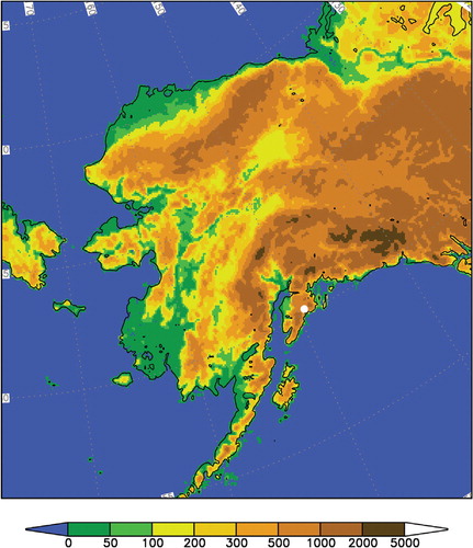
Bear Lake (60.21°N, 149.36°W) was selected for the sensitivity studies presented here, because it is one of the largest lakes within ALISON. Bear Lake is located 10 km north of Seward in the south-east of Alaska (Fig. 1). This lake is oriented from north to south with a maximum fetch of about 2.4 km. The mean water depth is 10 m.

Fig. 1.  Surface elevation [m] of the HIRLAM Alaska domain. In the south-east of Alaska the location of the Bear Lake is indicated in white.

There have been eight ice seasons of measurements at ALISON site so far. The extended winter season 2003/2004 can be regarded as an average winter season in terms of precipitation, temperature and snow and ice depth within the time period from 2003 to 2011, available from the ALISON (2011) dataset. It covers the longest time period among the available seasonal measurements. Additionally, the onset of ice melting is more pronounced than during the other periods. Therefore, we focus our modelling experiments on this winter.

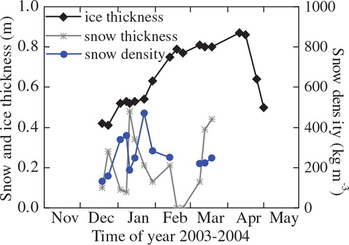
Figure 2 shows the observed snow and ice depth and snow density in Bear Lake in 2003/2004. The snow depth and density varies significantly. Snow mass increases after a snowfall event. Snow depth reduces while the snow density increases due to snow redistribution and compaction. The reduction of snow depth during cold season may also be linked with snow-to-ice transformation. For example, at the beginning of January, after a snowfall event, snow depth gradually decreases while the ice depth increases. Because the air temperature has been mostly well below the freezing point, it is unlikely that the decrease of snow depth is totally caused by melting. The decrease of snow mass is connected with slush formation and further refreezing to snow-ice. The last episode of ice growth may result from refreezing of melting snow, that is, superimposed ice formation. Overall, during early winter season, the presence of snow on ice does not strongly reduce the ice growth rate as expected by snow insulation effect. This also applies to other ALISON winter season observations (2004–2011).

Fig. 2.  Snow and ice depth and snow density measured on Bear Lake during the 2003/2004 ice season.

4. Setup of model experiments

4.1. Forcing data

HIgh Resolution Limited Area Model forecasts were run every 6 h from 1 November 2003 to 15 June 2004 to obtain the atmospheric forcing data. Since it is planned in the future to apply both FLake and HIGHTSI as parameterisations within operational NWP models, it is beneficial to test the stand-alone models driven by the atmospheric data from an NWP model.

HIgh Resolution Limited Area Model is a numerical short-range weather forecasting system, used operationally within the international HIRLAM programme partners of 11 European countries. HIRLAM is based on the hydrostatic primitive equations; the dependent variables are temperature, wind component, humidity, surface pressure, cloud water content and turbulent kinetic energy (Undén et al., 2002). We applied an experimental HIRLAM version close to v.7.3, which contains improved surface parameterisations. As a limited area model, HIRLAM requires lateral boundary conditions from global/hemispheric model, normally provided by the European Centre for Medium Range Weather Forecasting (ECMWF). For the present study, the lateral boundary conditions were taken from archived ECMWF analyses.

The HIRLAM experiment domain includes the whole continental area of Alaska (Fig. 1), which will enable us to consider also other lakes of the ALISON (2011) dataset in the future. HIRLAM forecasts were run with a horizontal resolution of 0.068° (~7.5 km) on a rotated latitude–longitude grid.

The 5-, 6- and 7-h forecasts of each HIRLAM simulation were saved. The instantaneous parameters (surface pressure as well as lowest model level temperature, specific humidity, u- and v-components) were extracted for the HIRLAM grid point nearest to Bear Lake from the 6-h forecasts. The accumulated parameters (snowfall, downwelling long-wave and direct and diffuse short-wave radiation) were calculated as differences between the 5- and 7-h forecasts to get values valid at every 6 h (00, 06, 12 and 18) coordinated universal time (UTC). It should be noted that HIRLAM may predict snowfall also at near-surface temperatures above 0 °C; for our FLake and HIGHTSI simulations, only snowfall at temperatures below 0.1 °C was considered.

A comparison with observation data from a meteorological station about 15 km north of Bear Lake (Seward: 60.3539°N, 149.3483°W; station ID USC00508377 from the U.S. National Climatic Data Center) shows a reasonable agreement of daily temperature and precipitation values. The HIRLAM temperature tends to be higher than the observed (bias: 1.8 °C) while the HIRLAM precipitation is lower than the observed (bias: −1.2 mm d⁻¹). However, it has to be taken into account that the meteorological station is further away from the sea and further up in the mountains compared to the lake, and that these differences could be genuine.

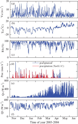
Figure 3 shows the time series of HIRLAM results that are used as external forcing for the lake ice models. Starting from mid-November (13 November), HIRLAM suggests cold conditions. The cold season extends until early April (7 April) when temperature slowly rises above the freezing point. The average temperature was −5.3 °C during the cold season (13 November–7 April) in contrast to +5.8 °C during the warm period (8 April–15 June). The HIRLAM wind speed seems to be related to temperature during these two periods. The cold temperature was accompanied by relatively large wind variations, while during the warm period the wind was weak. During the winter, the total HIRLAM snow precipitation falling when the 2-m temperature was less than 0.1 °C was 303 mm water equivalent compared to 306 mm water equivalent at the Seward station.

Fig. 3.  The forcing data from HIRLAM model; (a) wind speed; (b) air temperature; (c) relative humidity; (d) original snow precipitation from HIRLAM (blue) and snow precipitation for T2m < 0.1 °C (red); (e) downwelling short-wave radiation; and (f) downwelling long-wave radiation.

4.2. Setup of the FLake and HIGHTSI experiments

Both models were initialised on 3 November 2003 and continuously run until 15 June 2004. Due to the different nature of the models, it is necessary to initialise the water temperature in FLake while this is not the case for the ice and snow model HIGHTSI, which does not simulate the lake water. FLake simulations were initialised with a constant lake water temperature of 4 °C. The simulations were run in the framework of the SURFace EXternalized model (Salgado and Le Moigne, 2010). This surface model includes FLake as a lake module along with other modules for land, sea and urban areas. Since a lake fraction of 100% is assumed for the present simulations, the results are not influenced by any module other than FLake. Since HIGHTSI does not simulate the lake water, the sensible heat flux from water to ice cannot be calculated but is prescribed as F _w = 0.5 W m⁻². This simple approximation that has to be made in an uncoupled ice model has been further investigated in Yang et al. (2012, this issue). Sensitivity studies suggest that increasing the heat flux from water to ice would have the strongest impact on ice depth during the late ice season. For technical reasons a minimum snow and ice depth value has to be maintained during the whole simulation. The lake is regarded to be ice and snow free at all times at which this minimum value is not exceeded. The minimum value is exceeded, that is, ice and snow start to form, when freezing and snowfall occur. At the end of the ice season, snow and ice retain their initial values and the lake is considered to be ice free (Yang et al., 2012, this issue). The different experiments are summarised in Table 1.

5. Results

5.1. Snow and ice depth

Time series of the observed and FLake-simulated ice and snow depth are presented in Fig. 4. The reference FLake run (RF) gives the poorest ice depth compared with observations. The ice depth is significantly underestimated. This could be caused by the fact that snow is simulated too thick because the snow density close to 100 kg m⁻³ is too low. The temporal variation of snow depth is a result of snow fall and snow melting.

Fig. 4.  Observed and FLake-simulated snow and ice depth Hs and Hi. (a) Reference FLake run and sensitivity experiment S1; (b–d) sensitivity experiments S2–S4.

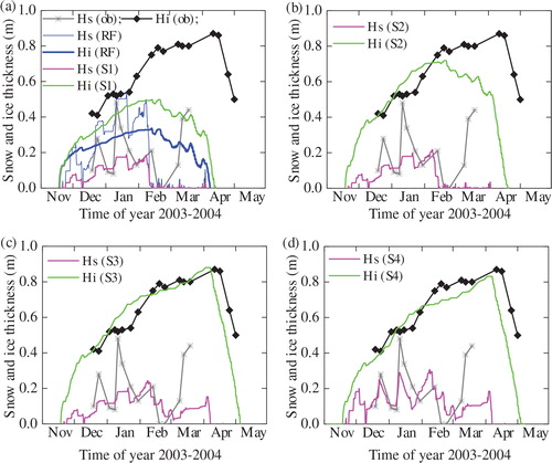
When a higher snow density of 320 kg m⁻³ is introduced (S1), the accumulated snow depth decreases. The insulation effect of snow is weakened and consequently the ice depth increases but the magnitude is still well below the observations. The heat conductivity in S2 is increased for thin snow layer. This modification leads to a much faster ice growth in early winter because snow insulation is largely reduced. In fact, this impact is so large that when snow is getting thicker in mid-winter, the ice is still growing strongly. Accordingly, the simulated total ice depth is in better agreement with observations until mid-February. In the second half of February, the mean air temperature is −1.6 °C and the downward solar radiation at the latitude of Bear Lake (60.21°N) is already notably large (~300 W m⁻²). Therefore, surface melting may occur and the surface albedo will change to 0.1 according to eq. (4). This will further enhance surface melting and eventually lead to a snow free condition. Since the albedo of melting ice is also set to 0.1, ice melts too early in spring.

A more reasonable snow and ice surface albedo set-up in S3 improves greatly the calculated ice depth. The temporal variability of snow is too low and the errors lie on high peaks of snowfall. The experiment S4 gives a similar ice growth than S3, with a slightly thinner ice appearing in mid-winter. The temporal snow variation is in a better agreement with the observations because observed snow density has been used.

The results of HIGHTSI sensitivity experiments are given in Fig. 5. Without snow, the seasonal maximum ice depth matches the observation but the phase considerably differs. Ice depth reaches a maximum value (0.84 m) around 9 February, while observation suggests a maximum (0.87 m) in spring (10 April). The onset of melting, defined as the start of monotonously decreasing sea ice depth, is simulated on 3 April, some 7 d earlier than observed. The simulated freeze-up date, defined as the appearance of lake ice, was 13 November and the simulated break-up date, defined as the total disappearance of lake ice, was 16 May. In reality the lake ice and snow might appear and disappear at different times in different areas of the lake, which cannot be considered in a one-dimensional lake ice model. Unfortunately there are no observations of freeze-up and break-up dates.

Fig. 5.  Observed and HIGHTSI-simulated snow and ice depth. (a–d) model experiments H1–H4.

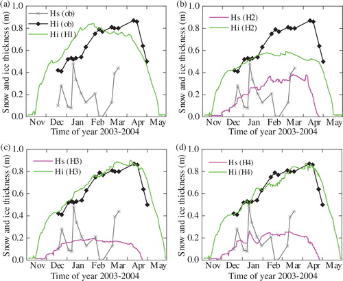
The snow insulation can reduce ice growth strongly as illustrated by experiment H2. In this case, the snow depth is calculated as a function of precipitation and densification as well as surface and subsurface melting. Until 12 February, the observed snow depth shows large variations while the simulated snow depth continuously increases. The model fails to reproduce two episodes of dramatic decrease of snow depth – in particular, the observed snow-free conditions on 18 and 23 February. Several factors could have led to the observed snow-free condition. The meteorological data suggest strong wind, which may have led to a redistribution of snow. During the second half of February, the downwelling solar radiation is already strong. It might not only melt the snow at the surface but also internally, leading to slush at the snow–ice interface. This slush layer may refreeze on the colder ice layer increasing its depth. Those effects can actually change the snow depth both from the top and from the snow-ice boundary and eventually lead to a snow-free condition.

Only small temporal snow depth variations (decrease/increase associated respectively with surface melting/snowfall) are simulated from mid-February onwards while the observations show a pronounced accumulation of snow at the end of February and beginning of March. The rapid melting of snow at the end of April is a result of albedo feedback mechanism, which is typically seen in high latitudes in early April when solar radiation increases significantly.

Compared to experiment H1, the ice freezing and break-up dates are about the same in experiment H2. In experiment H3, the decrease of snow depth is caused by formation of slush layer, surface and subsurface melting as well as densification. Differently from Cheng et al. (2006), we have applied a first-order approximation to let the slush layer (formed by positive freeboard due to heavy snow load or melting snow) to be refrozen totally. In this case, the simulated snow depth is much smoother compared to the result of H2. The snow-to-ice transformation results in larger ice depth leading to a good agreement with observations, especially during the growing phase up to the first half of April when snow is still present.

In H4 the onset of ice melt is simulated only 2 d later than observed. The development of sea ice depth is very well represented compared to the other HIGHTSI simulations. Decreasing snow depth along with increasing ice depth is simulated at several occasions (end of December to beginning of January as well as second and third week of January) in H4. This is due to the prescribed snow density from measurements, which varies largely in contrast to the smooth change, that is, a gradual increase from 320 to 450 kg m⁻³, in the parameterisation in experiments H2 and H3. The last observed snow growth episode in March is not comparable with the simulations (H2, H3 and H4). In reality the observed event may refer to heavy snowfall. Since we have applied HIRLAM results as external forcing, discrepancy between the observed and simulated by HIRLAM snow precipitation may lead to errors in the snow depth simulated by HIGHTSI. The effect of wind resulting in snow redistribution is not considered in HIGHTSI, which may introduce further inaccuracy to simulated snow depth.

Simple statistics of simulated versus observed snow and ice depth are given in Table 2. The statistics confirm that the more realistic parameterisations in the FLake sensitivity experiments and the inclusion of more physical processes in HIGHTSI generally improve the simulation. The FLake reference simulation shows large errors and small correlations. The ice depth correlation substantially improves from S2 to S3 when introducing the more realistic albedo values. The prescribed snow density in experiments S4 and H4 improves the correlation coefficients of snow depth compared to the other experiments; however, correlation coefficients are still very low indicating that snow depth is challenging to simulate even when prescribing the snow density. Except for the correlation coefficient of snow depth, the more complex HIGHTSI model shows smaller errors and higher correlations compared to the simpler FLake model.

Table 2. Bias, root mean square error (RMSE) and correlation coefficient of simulated snow and ice depths compared to observations. For the bias negative values indicate an underestimation by the models and positive values an overestimation

		RF	S1	S2	S3	S4	H1	H2	H3	H4
Bias (m)	Snow	−0.01	−0.13	−0.10	−0.10	−0.06	–	0.06	−0.04	−0.01
	Ice	−0.44	−0.32	−0.16	−0.03	−0.09	0.04	−0.13	0.05	0.01
RMSE (m)	Snow	0.21	0.20	0.20	0.18	0.15	–	0.15	0.14	0.13
	Ice	0.48	0.40	0.31	0.12	0.14	0.14	0.18	0.08	0.07
Correlation coefficient	Snow	0.23	0.23	0.23	0.28	0.42	–	0.17	0.23	0.36
	Ice	0.21	0.06	0.1	0.74	0.74	0.54	0.67	0.92	0.90

5.2. Snow and ice temperature

A comparison between observed and simulated surface temperature (snow or ice if snow is not present) is given in Table 3. Large errors seem to appear in the FLake experiments. A number of physical reasons could lead to large errors. In early January, the too cold surface temperature of RF is linked with too small snow density. Once the physical parameters of snow in FLake get improved with the experiments S1–S4, the temperature errors are reduced but are still large. On 22 January 2004, all model runs give small errors. This is because a melting surface is simulated that matches the reality. Therefore, the surface temperature difference is confined. In early spring, the RF gives an overestimation of surface temperature. This is associated with the unrealistically small albedo. A small albedo brings too much solar radiation down to the surface. The consequence is a too warm surface and too early onset of snow melting (Fig. 4a). With modified albedo values in S3 and S4, the surface temperature gets too cold in early spring. In spite of this, snow and ice still melt too early. Therefore, it can be concluded that an improvement of snow and ice properties in FLake without inclusion of more physical processes such as snow-to-ice transformation only improves the simulation of the surface temperature to some extent. In our case, improvements are restricted to the winter season.

Table 3. Comparison between simulated and measured surface temperatures (°C) for all model runs. The comparisons match the specific date and time of measurement (local noon). Bias, root mean square error (RMSE) and correlation coefficient are also given

		Temperature difference at surface: (T cal – T ob )
Date	T sfc (ob)	RF	S1	S2	S3	S4	H1	H2	H3	H4
18 December 2003	−4.3	−2.74	−1.26	0.01	−0.18	−0.73	0.31	−0.31	−0.22	−0.52
23 December 2003	−10.6	3.44	3.57	4.35	4.14	3.47	3.18	2.04	1.98	1.80
2 January 2004	−7.8	−18.03	−13.98	−7.91	−8.76	−8.25	−4.37	−6.39	−6.26	−6.49
7 January 2004	−9.0	−13.86	−12.81	−9.75	−11.06	−9.90	−3.72	−4.41	−5.15	−4.40
10 January 2004	−0.7	−0.09	0.08	−0.66	−1.20	−0.64	−1.75	−1.62	−1.39	−1.60
14 January 2004	−12.0	−1.72	−1.35	−0.89	−1.43	−1.44	1.82	−2.42	−2.31	−2.71
22 January 2004	−0.20	0.20	0.20	0.20	0.20	0.20	0.07	0.20	0.20	0.20
29 January 2004	−9.8	6.23	3.99	2.86	1.19	0.79	3.67	3.63	3.42	3.35
12 February 2004	−4.7	4.47	4.51	4.61	−1.09	−2.34	1.96	−0.45	0.26	−2.45
8 March 2004	−4.4	3.38	3.22	1.26	−4.84	−4.70	−0.39	−1.39	−0.28	−3.08
18 March 2004	−5.6	5.14	5.32	4.83	−4.98	−5.06	2.39	1.30	2.13	0.15
Bias		−1.23	−0.77	−0.10	−2.55	−2.60	−0.03	−0.89	−0.69	−1.43
RMSE		7.61	6.40	4.59	4.96	4.62	2.57	2.86	2.91	3.04
Correlation coefficient		0.55	0.62	0.69	0.68	0.72	0.82	0.81	0.82	0.81

HIGHTSI-simulated surface temperatures are generally closer to the observed values although the cold bias in early January still exceeds −5 °C. It should be noted that there are comparably little changes in the surface temperature errors between the four HIGHTSI experiments; in fact bias and RMSE even increase from H1 to H4. Improvements from H1 to H4 are restricted to snow and ice depth.

The snow–ice interface temperature (Table 4) is well simulated in the FLake reference and S1 simulations. Because of the relatively low snow heat conductivity in these two simulations the too cold temperatures at the surface do not strongly propagate to the snow–ice interface while this happens in S2–S4. HIGHTSI simulations generally show a good agreement in terms of the snow–ice interface temperature. The multilayer approach allows a detailed description of the heat transfer from the surface to the ice–water interface.

Table 4. Comparisons between simulated and measured temperature (°C) at the snow − ice interface for all model runs. The comparisons match the specific date and time of measurement (local noon). Bias and root mean square error (RMSE) are also given. Note that the experiment H1 is excluded because snow is not considered

		Temperature difference at snow–ice interface: (T cal – T ob )
Date	T sin	RF	S1	S2	S3	S4	H2	H3	H4
18 December 2003	−1.29	0.56	−0.42	−2.17	−2.33	−1.37	−0.59	−0.61	−0.26
23 December 2003	−0.75	0.32	−0.63	−3.08	−3.23	−1.36	−1.40	−1.43	−0.95
2 January 2004	−2.12	1.35	−0.14	−3.70	−3.92	−8.44	−1.12	1.14	−0.83
7 January 2004	−5.41	3.73	0.20	−7.38	−8.21	−7.84	0.42	0.36	0.68
10 January 2004	−0.22	0.17	0.09	−0.57	−0.89	−0.22	−2.22	−2.26	−1.75
14 January 2004	−1.32	0.56	−1.15	−5.33	−5.59	−3.77	−1.70	−1.73	−1.02
22 January 2004	−0.03	0.03	0.03	0.03	0.03	0.03	−1.26	−1.31	−1.29
29 January 2004	−2.18	1.93	0.88	−2.02	−2.95	−2.54	0.06	0.02	0.46
12 February 2004	−0.15	–	–	–	−3.42	−3.31	−0.03	−0.04	−0.03
8 March 2004	−1.01	–	–	–	−7.57	−7.24	0.34	0.30	0.47
18 March 2004	0.00	–	–	–	−8.46	−7.98	−0.44	−0.47	−0.35
Bias		1.08	−0.14	−3.03	−4.23	−4.00	−0.72	−0.76	−0.44
RMSE		1.36	0.50	3.24	5.04	5.08	1.10	1.13	0.88
Correlation coefficient		0.75	0.86	0.90	0.73	0.72	0.83	0.83	0.86

5.3. Comparison of FLake and HIGHTSI results

For both FLake and HIGHTSI, the differences between simulated and observed ice depth tend to be reduced when more physical processes are taken into consideration. In this section we focus on the comparison between best results of FLake (S4) and HIGHTSI (H4). The seasonal maximum ice depth can be simulated with a bias of −0.04 m for FLake and no bias for HIGHTSI. The calculated monthly mean snow and ice depths and ice growth rates are given in Table 5. Large differences of simulated snow depth show up in spring (March, April) probably due to the different treatment of downward solar radiation in FLake and HIGHTSI. FLake has only one snow layer and the solar radiation is assumed to heat the snow surface, conduct heat through the single snow layer and melt snow at the surface. HIGHTSI has 10 snow layers, the downward solar radiation is assumed to distribute exponentially down to the whole snowpack (Beer's law). Warming and melting is accounted for through the heat balance of surface layer (first snow layer on top) and snow internal warming and melting (caused by penetrating solar radiation). In HIGHTSI it can happen that only the uppermost snow layers are affected by melting, and the snow refreezes further down in the snow pack. Another reason for the difference in spring could be higher snow heat conductivity in FLake compared to HIGHTSI, which can lead to a more efficient warming of the snow-ice pack.

Table 5. Monthly mean of simulated ice depth and ice growth rate by FLake (S4) and HIGHTSI (H4)

	Simulated monthly mean snow depth (m)		Simulated monthly mean ice depth (m)		Simulated monthly mean ice growth rate (cm d^−1)
	S4	H4	S4	H4	S4	H4
November	0.06	0.02	0.12	0.21	1.0	1.3
December	0.14	0.11	0.36	0.42	0.5	0.4
January	0.16	0.19	0.58	0.58	0.6	0.4
February	0.17	0.23	0.69	0.69	0.2	0.3
March	0.09	0.24	0.76	0.81	0.4	0.2
April	0.03	0.11	0.56	0.81	−2.5	−0.7
May	0	0	0.03	0.31	0	−2.1

The simulated monthly mean ice depths are close to each other, especially in mid-winter (January–March). In April and May, the differences are increasing because of the different time of the onset of melting. This can be seen very clearly from ice growth rate, that is, FLake simulates the onset of melting (April) one month in advance compared with HIGHTSI (May). Nevertheless, a similar ice melting rate of the order of 0.02 m d⁻¹ is seen. However, S4 and H4 provide similar ice growth rate in other months. In November, H4 is practically snow-free which means that ice grows faster than in S4. In December, the difference between S4 and H4 is narrowed. In January, S4 suggests more ice growth while in February H4 grows faster. In March, the difference is increasing with more ice growth for S4.

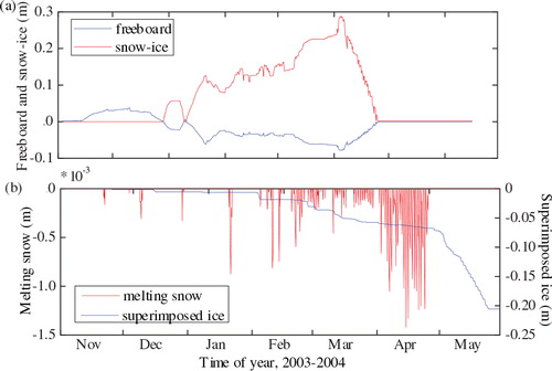
The ice growth is similar between FLake (S4) and HIGHTSI (H4) for different reasons. In S4, the effective snow heat conductivity (k _seff) is closely associated with the actual snow depth in FLake. Its value may be quite large (close to k _i), in particular when snow is thin therefore prompting ice growth. In H4, the ice growth is largely a result of the snow-ice formation. Fig. 6 shows HIGHTSI-simulated snow-ice and superimposed ice during the whole period. When snow is flooded (negative freeboard), the slush snow is refrozen to snow-ice. The formation of superimposed ice is more pronounced in early spring when melting snow refreezes at the snow surface and under it.

Fig. 6.  Snow-ice and superimposed ice simulated by HIGHTSI.

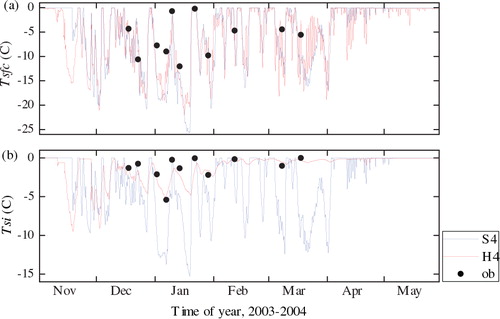
The observed time series and the time series of surface and snow–ice interface temperature simulated by S4 and H4 are shown in Fig. 7. FLake and HIGHTSI are able to catch temperature changes correctly, particularly for a warm surface. While the simulated surface temperature of FLake is very similar to that of HIGHTSI, the simulated snow–ice interface temperature is clearly colder in FLake than in HIGHTSI. In FLake, a strong heat flux through the snowpack is caused by the large effective snow heat conductivity.

Fig. 7.  The time series of observed (black points) and simulated surface temperature (T _sfc), snow–ice interface temperature (T _si) from S4 (blue line) and H4 (red line).

6. Summary and conclusions

Two numerical models (FLake and HIGHTSI) have been used to investigate snow and ice thermodynamics. Sensitivity experiments have been carried out for Bear Lake, close to Seward in the south-east of Alaska. This choice was made in order to have access to a comparably detailed data set on lake snow and ice depth and temperature, which is available from the ALISON (2011). HIRLAM forecasts over Alaska have been created and used to drive FLake and HIGHTSI. Special attention has been paid to the physical parameterisations of the thermal and optical properties of snow as well as to the snow-to-ice transformation process. We have assessed how realistically the snow accumulation and freezing and melting of the lake is treated in the models. The original parameterisations in FLake define a too small snow density, which may lead to a significant underestimation of ice depth. With the correction of albedo and snow density and with the inclusion of the effective snow heat conductivity, FLake results can be substantially improved. HIGHTSI results are substantially improved when the snow-to-ice transformation is taken into account.

Several parameters and processes have been found to be important for a realistic simulation of ice and snow:

• the snow density, which should be variable considering ageing and compacting of snow

• the snow heat conductivity, which is closely related to the snow density and for which inhomogeneities in the snow cover due to redistribution by wind or heterogeneous snow metamorphism should be considered

• the albedo of snow and ice, which strongly influences snow and ice melting in spring

• the transformation of snow into ice through flooding caused by strong snowfall on thin lake ice and refreezing, or through snow melting and refreezing

With the improvements the seasonal ice cover can be well simulated. The seasonal maximum ice depth is simulated with a bias of −0.04 m for Flake and with no bias for HIGHTSI. However, modelling of the snow depth is still a challenging task, especially during the growth of snow. This is because the increase of snow depth is strongly connected with the snowfall events, which are given as external forcing for FLake and HIGHTSI. The accuracy of snowfall prediction depends on the NWP model. On the other hand, in situ snow precipitation is also prone to errors, that is, the snow gauge tends to underestimate the local snow accumulation. Therefore, it is understandable that the models may contain large errors during the snowfall period. An additional complication may be added because of the wind drift as well as snow metamorphism affecting the snow density. Indeed, with a prescribed snow density the simulated results can be improved to some extent. In contrast, melting of snow is directly linked with thermodynamic processes handled by the snow/ice model. Therefore, there is potential to improve the simulation of snow depth in the melting season.

Overall, HIGHTSI gives more accurate surface temperature than FLake, as compared with the measurements. HIGHTSI applies an iterative procedure to calculate the surface temperature, while FLake applies a simpler approximation. Iteration can be considered an optimal method for surface temperature calculation. It may, however, be too expensive to be included in the snow and ice parameterisations for the current NWP models.

In future, the advantages of both FLake and HIGHTSI models could be combined by coupling the two models using HIGHTSI for the lake ice and snow simulation and FLake for the water underneath. This new model could be coupled to a NWP or climate model to simulate the real-time interaction between lakes and the atmosphere.

7. Acknowledgements

The third author (YY) was supported in early 2011 by a CIMO scholarship from Ministry of Education in Finland. The HIGHTSI modelling was supported by the National Natural Science Foundation of China (grant no. 51079021, 40930848) and the Norwegian Research Council (grant no. 193592/S30). The field data are courtesy of the ALISON (http://www2.gi.alaska.edu/alison/ALISON_pubs.html).The authors thank Dr. Ekaterina Kurzeneva for valuable discussions during the preparation of this manuscript. The suggestions by two anonymous reviewers led to significant improvements of the manuscript.

References

- ALISON. 2011. Alaska Lake Ice and Snow Observatory Network. Online at http://www.gi.alaska.edu/alison/ALISON_measures.html.
- Anderson, E. A. 1976. A Point Energy and Mass Balance Model of a Snow Cover. Technical Report NWS 19, 150 pp., Natl. Oceanic and Atmos. Admin., Washington, D. C.
- Ashton G. D. River and lake ice thickening, thinning and snow ice formation. Cold Regions Sci. Technol. 2011; 68: 3–19.
- Briegleb, B. P., Bitz, C. M., Hunke, E. C., Lipscomb, W. H., Holland, M. M. and co-authors. 2004. Scientific Description of the Sea Ice Component in the Community Climate System Model, Version Three. Technical Report NCAR/TN-463 + STR, National Center for Atmospheric Research, Boulder, CO, 78 pp.
- Bolsenga S. J. Preliminary observations on the daily variation of ice albedo. J. Glaciol. 1977; 18: 517–521.
- Brown L. C. Duguay C. R. The response and role of ice cover in lake-climate interactions. Prog. Phys. Geogr. 2010; 34: 671–704.
- Cheng B. Launianen J. Vihma T. Modelling of Superimposed ice formation and Sub-Surface melting in the Baltic Sea. Geophysica. 2003; 39: 31–50.
- Cheng B. Vihma T. Pirazzini R. Granskog M. A. Modelling of superimposed ice formation during the spring snowmelt period in the Baltic Sea. Ann. Glaciol. 2006; 44: 139–146.
- Cheng, B., Zhang, Z., Vihma, T., Johansson, M., Bian, L. and co-authors. 2008. Model experiments on snow and ice thermodynamics in the Arctic with CHINARE 2003 data. J. Geophys. Res., 113, C09020.
- Christensen J. H. Christensen O. B. A summary of the PRUDENCE model projections of changes in European climate by the end of this century. Clim. Change. 2007; 81: 7–30.
- Curry J. A. Schramm J. Perovich D. Pinto O. Application of SHEBA/FIRE data to evaluation of snow/ice albedo parameterizations. J. Geophys. Res. 2001; 106: 15345–15355.
- Duguay, C. R., Flato, G. M., Jeffries, M. O., Ménard P., Morris, K. and co-authors. 2003. Ice cover variability on shallow lakes at high latitudes: model simulations and observations. Hydrol. Proc. 17, 3465–3483.
- Ebert E. E. Curry J. A. An intermediate one-dimensional thermodynamic sea ice model for investigating ice-atmosphere interaction. J. Geophys. Res. 1993; 98(C6): 10085–10109.
- Eerola K. Rontu L. Kourzeneva E. Shcherbak E. A study on effects of lake temperature and ice cover in HIRLAM. Boreal. Env Res. 2010; 15: 130–142.
- Gabison R. A thermodynamic model of the formation, growth, and decay of first-year sea ice. J. Glaciol. 1987; 33: 105–109.
- Gardner, A. S. and Sharp, M. J. 2010. A review of snow and ice albedo and the development of a new physically based broadband albedo parameterization. J. Geophys. Res. 115, F01009, doi:10.1029/2009JF001444.
- Henneman H. E. Stefan H. G. Albedo models for snow and ice on a freshwater lake. Cold Regions Sci. Technol. 1999; 29: 31–48.
- Heron R. Woo M. K. Decay of a High Arctic lake-ice cover: observations and modelling. J. Glaciol. 1994; 40: 283–292.
- Huwald H. Tremblay L.-B. Blatter H. Reconciling different observational data sets from Surface Heat Budget of the Arctic Ocean (SHEBA) for model validation purposes. J. Geophys. Res. 2005; 110: C05009.
- Jeffries M. O. Morris K. Instantaneous daytime conductive heat flow through snow on lake ice in Alaska. Hydrol. Proc. 2006; 20: 803–815.
- Jeffries M. O. Morris K. Duguay C. R. Lake ice growth and decay in central Alaska: observations and computer simulations compared. Ann. Glaciol. 2005; 40: 195–199.
- Kawamura T. Ohshima K. I. Takizawa T. Ushio S. Physical, structural, and isotopic characteristics and growth processes of fast sea ice in Lutzow-Holm Bay, Antarctica. J. Geophys. Res. 1997; 102(C2): 3345–3355.
- Kitaigorodskii S. A. Miropolsky Y. Z. On the theory of the open ocean active layer. Izv. Akad. Nauk SSSR. Fizika Atmosfery I Okeana. 1970; 6: 178–188.
- Launiainen J. Cheng B. Modelling of ice thermodynamics in natural water bodies. Cold Reg. Sci. Technol. 1998; 27(3): 153–178.
- Leppäranta M. A growth model for black ice, snow ice and snow thickness in subantarctic basins. Nordic Hydrol. 1983; 14: 59–70.
- Liu J. Zhang Z. Inoue J. Horton R. M. Evaluation of snow/ice albedo parameterizations and their impacts on sea-ice simulations. Int. J. Climatol. 2007; 27: 81–91.
- MacKay, M. D., Neale, P. J., Arp, C. D., De Senerpont Domis, L. N., Fang, X., and co-authors. 2009. Modeling lakes and reservoirs in the climate system. Limnol. Oceanogr. 54, 2315–2329.
- Maykut G. A. Untersteiner N. Some results from a time-dependent thermodynamic model of sea ice. J. Geophys. Res. 1971; 76: 1550–1575.
- Mironov, D. V. 2008. Parameterization of Lakes in Numerical Weather Prediction. Description of a Lake Model. Technical Report of COSMO, No. 11. Deutscher Wetterdienst, Offenbach am Main, 41 pp.
- Mironov, D., Heise, E., Kourzeneva, E., Ritter, B., Schneider, N. and co-authors. 2010. Implementation of the lake parameterization scheme FLake into the numerical weather prediction model COSMO. Boreal Env. Res. 15, 218–230.
- Nicolaus M. Haas C. Bareiss J. Observations of superimposed ice formation at melt-onset on fast ice on Kongsfjorden, Svalbard. Phys Chem Earth. 2003; 28: 1241–1248.
- Perovich, D. K. 1996. The optical properties of sea ice. CRREL Monogr. 96–1, 25 pp.
- Prowse T. D. Marsh P. Thermal budget of river ice covers during break-up. Can. J. Civil Eng. 1989; 16: 62–71.
- Salgado R. Le Moigne P. Coupling of the FLake model to the Surfex externalized surface model. Boreal Env. Res. 2010; 15: 231–244.
- Samuelsson P. Kourzeneva E. Mironov D. The impact of lakes on the European climate as simulated by a regional climate model. Boreal Env. Res. 2010; 15: 113–129.
- Stepanenko, V. M., Goyette, S., Martynov, A., Perroud, M., Fang, X. and co-authors. 2010. First steps of a Lake Model Intercomparison Project: LakeMIP. Boreal Env. Res. 15, 191–202.
- Sturm M. Holmgren J. König M. Morris K. The thermal conductivity of snow. J. Glaciol. 1997; 43: 26–41.
- Sturm M. Liston G. E. The snow cover on lakes of the Arctic Coastal Plain of Alaska. J. Glaciol. 2003; 49(166): 370–380.
- Sturm, M., Perovich, D. K. and Holmgren, J. 2002. Thermal conductivity and heat transfer through the snow and ice of the Beaufort Sea. J. Geophys. Res. Oceans 107(C21), 8043, doi:10.1029/2000JC000409.
- Undén, P., Rontu, L., Järvinen, H., Lynch, P., Calvo, J. and co-authors. 2002. The HIRLAM-5 scientific documentation. 144pp. Online at http://hirlam.org and SMHI, S-60176 Norrköping, Sweden.
- Vavrus S. J. Wynne R. H. Foley J. A. Measuring the sensitivity of southern Wisconsin lake ice to climate variations and lake depth using a numerical model. Limnol. Oceanogr. 1996; 41: 822–831.
- Yang, Y., Leppäranta, M., Cheng, B., Li, Z. and Rontu, L. 2012. Numerical modelling of snow and ice thicknesses in Lake Vanajavesi, Finland. Tellus, 64A, 17202.