Modelling the re-intensification of tropical storm Erin (2007) over Oklahoma: understanding the key role of downdraft formulation

ABSTRACT

This article reports on the inland re-intensification of tropical storm (TS) Erin (2007). In this research, the physical processes that resulted in the re-intensification of TS Erin over Oklahoma, USA, on 19 August 2007 was determined and a sensitivity study on microphysics, planetary boundary layer and convective parameterisation schemes was performed in the mesoscale modelling system, MM5. Also, we diagnosed and explained the remarkable difference between model behaviour of the original Kain–Fritsch 1 (KF1) scheme and its revised counterpart (KF2). The numerical results showed only modest sensitivity to the selected microphysics schemes – the relatively simple ‘Simple Ice’ and the advanced Reisner-Graupel. We found a relatively high sensitivity to the selected boundary layer parameterisation. Enhanced mixing in the medium range forecast (MRF) scheme leads to a relatively small convective available potential energy (CAPE), a deeper boundary layer and a lower dew point temperature, thus to a relatively stable environment. Therefore, MRF forecasts less precipitation (up to 150 mm) than the local mixing scheme, ETA. Model results appeared most sensitive to the selected convection schemes, that is, Grell, KF1 and KF2. With Grell and KF1, Erin intensifies and produces intense precipitation, but its structure remains close to a mesoscale convective system (MCS) or squall line rather than of the observed tropical cyclone. Both schemes also simulate the most intense precipitation too far south (100 km) compared to observations. On the contrary, KF2 underestimates precipitation, but the track of the convection, the precipitation and the pressure distribution are relatively close to radar and field observations. A sensitivity study reveals that the downdraft formulation is critical to modelling TS Erin's dynamics. Within tropical cyclogenesis, the mid-level relative humidity (RH) is generally very high, resulting in very small downdrafts. KF2 generates hardly any downdrafts due to its dependence on mid-level RH. However, KF1 and Grell generate much stronger downdrafts because they both relate the downdraft mass flux (DMF) to vertical wind shear. This larger DMF then completely alters TS Erin's dynamics. A modified version of the Grell scheme with KF2 RH-dependent downdraft formulation improved the simulation considerably, with better resemblance to observations on trajectory, radar reflectivity and system structure.

• Erin
• tropical storm
• re-intensification
• MM5
• parameterisation
• downdraft
• convection
• precipitation efficiency

1. Introduction

Tropical storm (TS) Erin developed in the Gulf of Mexico on 14 August 2007 from a persistent area of convection. Erin made landfall near Lamar, Texas, USA, on 16 August 2007. Subsequently, TS Erin quickly weakened to a tropical depression with wind speeds of ~30 km h⁻¹. Surprisingly, around 9:30 UTC on 19 August 2007, Erin gained an eye-like structure. Erin re-intensified dramatically over Oklahoma City, with maximum sustained winds of 90 km h⁻¹ and gusts up to 120 km h⁻¹. The 24-h accumulated precipitation amounted to 100–200 mm widespread over Oklahoma, with unofficial observations reporting up to 280 mm. The intense precipitation, flooding and wind gusts caused extensive damage (more than $22 million) and resulted in at least seven casualties.

Usually, tropical cyclones (TCs) weaken after landfall, when they get disconnected from their main energy provision, that is, warm sea water (>26°C), and experience vorticity spin-down by increased surface friction. Occasionally, such systems intensify over land when remnants experience extratropical transition in a baroclinic zone further north (Evans and Hart, 2003). Sometimes remnants of TCs and TSs intensify without a baroclinic zone in the direct proximity, for example, TS Allison and Chantal in 1989, hurricane Danny in 1997 and hurricane Allison in 2001 (Kong and Gedzelman, 2004). However, re-intensification as far inland as Oklahoma (>800 km) is generally rare. A second unique aspect of this study is the availability of a dense network of surface observations in the study area, that is, the Oklahoma Mesonet.

We analysed the redeveloped TS Erin using the mesoscale model, MM5, which has often been used in hurricane modelling (Braun and Tao, 2000; Rao and Prasad, 2007; Pattnaik and Krishnamurti, 2007; Srinivas et al., 2007) and severe convective storms with intense precipitation (Wisse and Vilà-Guerau de Arellano, 2004, henceforth WV04). These studies indicated that the model results were relatively sensitive to the selected parameterisation schemes, which motivated us to investigate analogue model sensitivity for TS Erin. Although hurricane forecasts with numerical weather prediction (NWP) models have improved substantially since the 1990s, further development in this area is required. For example, the mean forecast errors of the Atlantic hurricane season 2007 were considerably above (25%) the 5-yr means (Brennan et al., 2009), probably because this season covered many hurricanes with rapid strengthening, analogue to the re-intensification of TS Erin. Hence, the aim of this article is threefold, that is, to:

• identify the physical processes that triggered the re-intensification of TS Erin.

• perform a sensitivity study on the model skill for different permutations of selected boundary layer, convection and microphysics schemes.

• understand the key role of different aspects of the convection scheme within the reference and revised KF scheme.

The case description and the experimental set-up are discussed in depth in Section 2. A description of the relevant parameterisations and their performance review along with a description of the model modifications is presented in Section 3. Section 4 describes the model results and interpretation, whereas Sections 5 and 6 present the discussion and conclusions, respectively.

2. Case description and experimental set-up

2.1. Case description

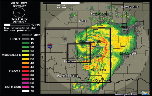
On 16 August 2007, around 10:30 UTC, the eye of TS Erin made landfall near Lamar, Texas, USA. After landfall, the system weakened to a tropical depression and on 17 August, 12:00 UTC, the system was classified as a ‘remnant low’. In the morning of 19 August, around 4:00 UTC, the system re-intensified abruptly over Oklahoma City, USA, with increased thunderstorm activity and precipitation. Maximum sustained wind speeds increased from 8 to 25 ms⁻¹ with wind gusts of up to 35 ms⁻¹ (Knabb, 2008). The system gained structure and radar observations showed an eye-like structure between 9:50 and 13:00 UTC (Fig. 1). At 00:00 UTC on 20 August, the circulation had dissipated and convection was widespread.

Fig. 1.  Radar reflectivity (dBZ) of the ‘eye’ of TS Erin 19 August 2007, 12:31 UTC. The squares indicate model domains 2 and 3. Source: wunderground.com.

Erin's sudden re-intensification was primarily caused by two processes. First, an upper-level short-wave trough translated from west to east, causing isentropic lifting and advection of positive vorticity. Second, when it arrived in Oklahoma, a band of warm–moist advection in the lower levels developed along the east flank of TS Erin with wind speeds of up to 20 ms⁻¹ (Arndt et al., 2009). With this band, the low-level wind speeds increased, while the upper-level winds remained constant. This decreasing wind speed with height is, amongst others, a characteristic property of warm core systems (Bosart and Bartlo, 1991). Collocation of high potential temperature with the surface low pressure, collocation of the surface mass convergence fields with the centre of TS Erin at each level and vertical stacking of the lows at successive heights indicate that TS Erin was a warm core system (Monteverdi and Edwards, 2008).

When the remnants of this warm core system interacted with the band of warm–moist advection, the system destabilised, reaching CAPE values of 1.9×10³ J kg⁻¹ (Arndt et al., 2009). This, combined with the isentropic lifting, resulted in an explosive growth of convection. Consequently, Erin intensified quickly during this burst of convection, resulting in the squall line wrapping around the circulation centre, and formed an eye-like structure (Fig. 1). The lowest observed central pressure during the re-intensification amounted to 1001.3 hPa, that is, 2 hPa lower than Erin's minimum pressure offshore (Knabb, 2008). When the upper-level short-wave trough moved further east, and the circulation centre of Erin moved further northeast, Erin became less structured and started dissipating.

Monteverdi and Edwards (2008) and Arndt et al. (2009) hypothesised that prior to TS Erin's arrival, the historically large rainfall amounts contributed to its intensification. Dew point temperatures were 4°C higher than Augusts’ climatological means, providing moist conditions and creating a less hostile environment for cyclogenesis (Emanuel, 2007).

2.2. Experimental set-up

Version 3.6.1 of the non-hydrostatic Penn State/NCAR Mesoscale Model MM5 (Dudhia, 1993; Grell et al., 1995) was used to conduct a 90-hour simulation over a research area centred over Oklahoma City, USA (Fig. 1). The simulation started on 17 August 2007, at 00:00 UTC, and finished on 20 August, at 18:00 UTC. The first 24 hours were considered as model spin-up and were therefore excluded from the analysis. Three two-way nested domains were defined, each with 31×31 grid points, with grid lengths of 27, 9 and 3 km, respectively, for domains 1, 2 and 3. Although this domain size may appear relatively small, a sensitivity analysis to the domain size revealed that a larger domain (51×51 grid points) resulted in a delay of Erin's arrival over Oklahoma and gave worse results compared to the smaller domain (31×31), that is, Erin did not intensify as much as with the smaller domain size and not as much as in reality. This was further confirmed by independent weather research and forecasting model (WRF) simulations with a large domain. As such, domain size affects the dynamics and large scale meteorological synoptic patterns. However, our study focuses on the physical rather than the dynamic aspect of Erin. Therefore, we aim to keep our analysis close to the analysed large-scale meteorological pattern, which is reflected best by a relatively small domain in this case. The initial and boundary conditions were obtained from 6-hourly operational analyses supplied by the European Center for Medium Range Weather Forecasts. A total of 33 σ-levels were defined, with a finer resolution in the atmospheric boundary layer (PBL).

Here, we report the results of two experiments. In the first experiment, MM5 was evaluated against observations for eight permutations of parameterisation schemes (Table 1). The sensitivity analysis covered two microphysics schemes, that is, the relatively basic ‘Simple Ice’ scheme (Dudhia, 1989) and the sophisticated ‘Reisner Graupel’ scheme (Reisner et al., 1998). Also, two PBL schemes were selected, that is, the local ETA scheme (Janjić, 1994) and the non-local MRF scheme (Hong and Pan, 1996). Concerning convection, the Grell (Grell 1993) and Kain–Fritsch 2 (KF2, Kain and Fritsch, 1993; Kain, 2004) schemes were utilised. During the study, it appeared that convection was not explicitly resolved adequately in the innermost domain; therefore, the convection scheme was also used in domain 3.

Table 1. Experimental set-up of experiment 1

	Run	CPS	PBL-scheme	Moisture-scheme
1	KMS	KF2	MRF	Simple Ice
2	KES	KF2	ETA	Simple Ice
3	KER	KF2	ETA	Reisner Gr
4	KMR	KF2	MRF	Reisner Gr
5	GMS	Grell	MRF	Simple Ice
6	GES	Grell	ETA	Simple Ice
7	GER	Grell	ETA	Reisner Gr
8	GMR	Grell	MRF	Reisner Gr

The second experiment consisted of a detailed analysis of the role of different physical aspects of the original KF and KF2 schemes. More precisely, we studied the sensitivity to shallow convection in KF2 and the formulation of the cloud radius, minimum cloud depth, CAPE, the minimum entrainment rate, the downdraft origination level (DDOL) and downdraft closure within both schemes (Table 2). The modifications are described in Section 3.2.3 (description KF2), where the modification number (Table 2, row 4) corresponds to the modification number in Section 3.2.3.

Despite MM5 currently being replaced by WRF, our results and insights are still valuable for a broad mesoscale model users’ community, since many of the evaluated schemes are still available in several models (e.g. WRF), and the obtained insights remain relevant for future modelling studies.

3. Model physics

Model performance relies on the quality of, amongst others, the parameterisation of subgrid processes. This section briefly describes the utilised schemes and reviews their typical performance.

3.1. Planetary boundary layer schemes

Vertical turbulent diffusion directly affects the distribution of moisture, heat and momentum from the surface to elevated levels in the troposphere. Hence, the PBL turbulence largely influences our daily near-surface weather. From the available schemes in MM5, ETA and MRF have been selected.

3.1.1. ETA.

ETA is a so-called 1.5 order as it uses the local vertical gradients of potential temperature, wind and the local Richardson number (Ri) to estimate the vertical transport (Mellor and Yamada, 1974; Janjić, 1994). ETA explicitly solves the prognostic turbulent kinetic energy (E) equation to quantify the turbulence and mixing intensity. Thus, the turbulent fluxes were estimated with a diffusion approach, , and the eddy diffusivity , with x being moisture, heat or momentum, f(Ri) a function that counts for stability effects and l a length scale defined as . In particular, the length-scale formulation is under scientific debate for this class of schemes (Cuxart et al., 2006).

3.1.2. MRF.

MRF is a first-order ‘non-local’ scheme as it does not only use the local gradients and Ri but also the PBL bulk characteristics to account for transport by eddies of a size close to the PBL height (Troen and Mahrt, 1986; Holtslag and Boville, 1993; Hong and Pan, 1996). MRF uses a pre-defined shape K _x (z/h), with h being the PBL height. Fluxes are calculated , where γ _x is the ‘counter gradient’ term. Because of this extra term, vertical mixing is more intense in MRF than in ETA.

3.1.3. Expectations and previous research.

WV04 examined the model sensitivity to the selection of MRF or ETA on a convective storm in the northeast of Spain. Then, MRF forecasted the highest precipitation amount, but the rainfall was spatially more widely distributed than with ETA, which forecasted the highest peaks in precipitation. Also, Braun and Tao (2000) studied the role of four PBL schemes with Hurricane Bob, including MRF and ETA. In that study, MRF behaved differently from the other schemes, with a dryer PBL, a higher cloud base and a smaller low-level convergence than with ETA. This resulted in a weaker hurricane with MRF compared to ETA.

In general, MRF produces enhanced mixing because of the counter gradient transport, with deeper PBLs, and more uniform daytime heat and moisture profiles. By contrast, in ETA, the vertical mixing is smaller than in MRF, which results in less widespread precipitation, more moisture in the lower levels of the troposphere, lower lifting condensation level (LCL) and higher CAPE, that is, more instability. When this instability is triggered by the convection scheme, it will produce heavy rainfall events locally. Hence, it was hypothesised that MRF will produce more widespread precipitation with smaller extreme values than ETA.

3.2. Cumulus Parameterisation Schemes (CPS)

Deep convection redistributes heat, moisture and momentum, and results in latent heat releases because of cloud condensation. The latter is very important as it is the primary energy source for convective systems, such as a MCS or a tropical cyclone.

Within the NWP models, the CPS design can be divided into three different parts. First, the dynamic control determines timing, location and intensity of convection. Second, the static control determines the net effect of the convection on the atmosphere, that is, how the vertical profiles will develop after convection has occurred. The third part determines the properties of the parameterised clouds.

3.2.1. Grell.

Grell is a relatively simple deep level control CPS (Grell 1993; Stensrud, 2007) based on a mass-flux formulation. On deciding whether convection is triggered, the scheme searches for the layer with the highest moist static energy. From this layer, convection will start if the LCL is within 50 hPa of the LFC, the so-called ‘lifting depth trigger’, and the parameterised cloud has a minimum thickness of 150 hPa. The intensity of the convection is determined by the ‘quasi-equilibrium assumption’, which implies that an air column is stabilised by convection at the same rate as it is destabilised by large-scale flow. The precipitation PR that arrives at the ground is calculated by , where I ₁ is the (normalised) integrated condensate in the updraft, m _b the mass flux at cloud base and 1−β the precipitation efficiency (PE). This PE dictates the fraction of the integrated condensate (generated in the updraft), which falls to the ground as convective precipitation and is a function of vertical wind shear, where increased wind shear results in decreased PE. The downdraft mass flux (DMF) (m ₀) is calculated by , where I ₂ is the normalised evaporation from the downdraft. In this way, m ₀ is a function of the updraft mass flux (UMF) and re-evaporation of convective condensate, which in turn depends on vertical wind shear. In the second part of the research, the Grell scheme is modified for a sensitivity analysis (labelled as modification nr. 8). The DMF is then calculated similarly as in KF2 (see Section 3.2.3), resulting in and Herein, RH_DSL is the average relative humidity (RH) of a 150 hPa thick layer, which begins from the starting level of the updraft.

3.2.2. KF1.

In terms of model hierarchy, the KF1 scheme can be considered as more sophisticated than Grell because of its more detailed treatment of entrainment and detrainment and trigger function (Kain and Fritsch, 1993). Stensrud (2007) categorises KF1 as a ‘low-level control’ convection scheme. The KF scheme consists of a number of ingredients that we will study later on. To decide on triggering convection, KF1 searches for an updraft source layer (USL), which must be at least 60 hPa deep. Hence, KF1 first mixes several model layers until it reaches the minimum depth. Because large-scale vertical motions often support convection, the mean USL temperature is increased with a temperature perturbation, which is proportional to the large-scale vertical motion. If the USL plus the perturbation temperature at its LCL are warmer than the ambient temperature at LCL, the USL parcel is released at its LCL with its original temperature. If this parcel reaches a minimum cloud depth of 3 km, deep convection is triggered. Without triggered convection, the scheme will move the USL slightly higher and the process is repeated. This continues between the ground and 300 hPa above the ground. If triggered, the cloud function calculates the updraft, downdraft and the associated mass flux. However, entrainment and detrainment are possible over the whole cloud depth – the lateral entrainment. As a closure, KF1 eliminates the CAPE (undiluted ascent) by at least 90% in an advective time period. This period varies between 30 and 60 min, depending on the mean wind speed between LCL and 500 hPa. The precipitation at the ground is given by the function PR=(1 − β)S, where PE equals (1−β) and S the sum of all the fluxes of water vapour and liquid water towards the updraft, 150 hPa above the LCL. The PE is inversely proportional to vertical wind shear (Marwitz, 1972; Foote and Fankhauser, 1973) and cloud base height (Zhang and Fritsch, 1986). The part of S that doesn't fall as precipitation is used to ‘fuel’ the DMF through evaporation, thus dictating the magnitude of the DMF.

3.2.3. KF2.

Based on a number of reported deficiencies in the KF1 scheme, Kain (2004) revised the original KF scheme on several aspects.

Modification 1: Shallow (non-precipitating) convection has been introduced as this affects the vertical atmospheric structures and plays a role in the timing of deep convection initiation. The latter is usually problematic in current generation of NWP and climate models (e.g. Rio et al., 2009). If all criteria for deep convection are fulfilled, except the minimum cloud depth, then shallow convection is activated.

Modification 2: The minimum cloud depth for deep convection is no longer fixed as in KF1 but has been made variable. The minimum cloud depth ranges between 2 and 4 km depending on T _LCL, where an increasing T _LCL will increase the cloud depth.

Modification 3: The CAPE is computed with a diluted parcel in KF2 (instead of undiluted parcel in KF1), which results in smaller CAPE yielding smaller mass fluxes and thus less convective intensity and precipitation.

Modification 4: The cloud radius is no longer fixed as in KF1 but has been made variable. The cloud radius (R) ranges from 1 to 2 km, depending on the vertical velocity at the LCL. Herein, an increasing vertical velocity results in an increasing cloud radius, which in turn will decrease the maximum possible entrainment rate (eq. 5 from Kain, 2004).

Modification 5: A minimum entrainment rate was included to circumvent the overestimated spatial spread of precipitation and the underestimated maximum rainfall.

Modification 6: The DDOL has been fixed at 150 hPa above the top of the USL, whereas it originally started at the level of minimum θ_es. The original DDOL was quite variable (300–850 hPa), which resulted in either tall and skinny downdrafts (high DDOL) or short and fat downdrafts (low DDOL). This influences the parameterised heating and drying rates in a way which is inconsistent with research on this topic.

Modification 7: The new downdraft is a mass-weighted mixture of air from each model layer within the downdraft source layer (DSL), which in KF2 extends from the DDOL to the top of USL. Originally, the scheme extracted most of the downdraft mass from a single origination level. Also, now the precipitation is determined by the residual condensate remaining after updraft detrainment and downdraft evaporation. The ratio DMF/updraft mass flux (DMFFRC) has been made RH dependent and is calculated by DMFFRC=2(1−RH_DSL), where RH_DSL is the mean RH within the DSL. Thus, the dependency on vertical wind shear and cloud base height is replaced by a dependency on RH, which is a key variable in determining rainwater evaporation and, as a consequence, also for PE (Ferrier et al., 1996) and downdraft strength (Knupp and Cotton, 1985).

3.2.4. Expectations and previous research.

Wang and Seamon (1997) examined the performance of KF1 and Grell, both in winter as well as summer with MM5. Both schemes overestimated rainfall minima and underestimated precipitation maxima. Despite the latter, KF1 forecasts appeared superior over Grell results. Considering the re-intensification of TS Allison (2001, Louisiana), Grell-MRF forecasts were closest to the observations and hence outperformed Grell-ETA and KF1-MRF (Kong and Gedzelman, 2004). Grell-MRF successfully reproduced convection east of the storm with the best results for both radar reflectivity and pressure distribution, although its squall line did not wrap around the cyclone centre as was observed. Liang et al. (2007) diagnosed drastically different, and regionally dependent, diurnal patterns with Grell or KF1. The Grell scheme realistically simulated the nocturnal precipitation maxima (large-scale tropospheric forcing) and their associated eastward propagating convective systems over the Great Plains, whereas the KF1 scheme produced more accurate results for the late afternoon peaks (near-surface forcing) in the southeast United States. In Bhaskar and Prasad (2006), KF2 outperformed both KF1 and Grell with the tropical cyclone intensification in Orissa in 1999. Both KF1 and Grell failed to let the system intensify sufficiently, whereas KF2 results agreed with observations. In Srinivas et al. (2007), Grell performed well at the onset of the intensification of cyclone in Andhra but failed to reproduce further cyclone deepening. In that case, KF2-ETA forecasted the most intense storm, whereas KF2-MRF forecasted a system that was closest to the observed intensity and trajectory.

In summary, earlier research shows no clear preference between KF1 and Grell, but in two mentioned case studies, KF2 outperformed Grell and in one KF2 outperformed KF1. Therefore, KF2 is expected to perform better then KF1 and Grell.

3.3. Microphysics schemes

MM5 offers a number of microphysics schemes of different complexities. Because it will appear later that the forecasts of Erin are only marginally sensitive to the choice of the microphysics schemes, only a very limited description of their physical background is reported. We use the Simple Ice and the advanced Reisner Graupel schemes.

Simple Ice (Dudhia, 1989) covers five water phases, that is, water vapour, cloud droplets, rain, ice crystals and snow, with phase transitions immediately at 0°C, whereas Reisner Graupel (Reisner et al., 1998) is a ‘mixed phase’ scheme, with ice crystals, cloud droplets, snow and rain, gradual rather than instantaneous transitions between the different phases.

3.3.1. Expectations and previous research.

Reisner et al. (1998) indicated that the assumption of a fixed number concentration for cloud ice and graupel in Simple Ice resulted in too much snow and graupel, whereas Reisner Graupel improved the forecast substantially. Chien and Jou (2004) found only a small sensitivity to the combined influence of different CPS's and moisture schemes in the Mei-Yu season (Taiwan). For convective summer days over the United States, Liu and Moncrieff (2007) found that mixed-phase schemes in general outperformed the Simple Ice scheme, with better precipitation distribution and timing. Considering the deep convection and strong vertical motions within TS Erin, we expect more advanced moisture schemes to be advantageous, although their sensitivity is probably smaller than for the PBL and CPS schemes.

4. Results and discussion

In this section, we will present the model results to get an overview of our findings (Sections 4.1 and 4.3), and the analysis and synthesis appear in Sections 4.2 and 4.4.

4.1. Results of experiment 1

4.1.1. Precipitation.

The main societal and economic impact of TS Erin was because of intense precipitation, which is therefore an important variable for model verification and sensitivity studies. Hence, we present the spatial distribution of the cumulative precipitation for the eight runs in Figs. 2 and 3. Also, Fig. 4a shows the precipitation accumulated over the maximum value per time step within domain 2. This domain has been selected because it covers a large part of Erin's re-intensification. We follow a strategy to accumulate the maximum precipitation value per time step (1 hour) to evaluate the model's capacity to produce the most intense precipitation, apart from the question whether the system's track is correctly forecasted. The observations originate from the Oklahoma Mesonet (Brock et al., 1995; McPherson et al., 2007) and are the maximum values per time step taken of a total of 31 weather stations distributed over domain 2.

Fig. 2.  Cumulative precipitation of all the 8 runs from August 17th 00:00 UTC to August 20th 18:00 UTC 2007, domain 2.

Fig. 3.  Observed precipitation (inches) from the Oklahoma Mesonet from August 18–19, 2007.

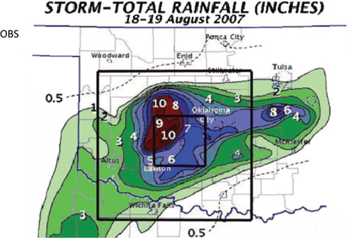
Large differences in forecasted cumulative precipitation occur, with the most distinct differences between KF2 and Grell (Figs. 2 and 4a). Grell-runs forecast substantially more precipitation than the KF2-runs, with differences up to 230 mm (GER–KER). Grell-runs evidently match the observed cumulative precipitation and the precipitation rate closer than KF2, whereas GER and GES overestimate the cumulative precipitation. All runs, and especially GES and GER, produce the most precipitation ~100–150 km spatially too far south. A second distinct difference occurs between the MRF and ETA-runs. Importantly, Grell-ETA forecasts 100 mm more cumulative precipitation than the other runs (Fig. 2). With KF2, the difference is smaller, but ETA still produces substantially more cumulative precipitation than MRF. This is consistent with results of WV04.

Fig. 4.  (A) Modelled and observed cumulative precipitation. The accumulation is performed over hourly maximum precipitation and (B) modelled and observed maximum wind speed. Both figures are in the period 18–19 August 2007, with time in UTC and from domain 2.

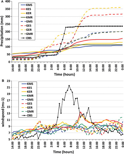
A striking feature is the increased precipitation of the Grell-ETA runs around 18 August, at 22:00 UTC, whereas the Grell-MRF runs hardly produced any precipitation (Fig. 4a). This sharp increase in precipitation corresponds with the isolated peaks of cumulative precipitation in Fig. 2 indicated by ‘A’. The differences in model formulation between ETA and MRF cause the CPS to initiate deep convection with ETA, but not with MRF. The relatively strong vertical mixing by the MRF scheme enhances the boundary layer depth and dry air entrainment, creating relatively lower near-surface dew point temperatures, and thus relatively less unstable conditions. As an illustration, considering 18 August 2007, 22:00 UTC, the forecasted soundings by GER has a higher dew point temperature and a lower LCL than the sounding by GMR (not shown). With GMR CAPE equals zero, there is no LFC, and consequently deep convection is inhibited. On the contrary, because of the lower and moister PBL in GER, convection is triggered resulting in an increase of cumulative precipitation. Erin's re-intensification started between 4:00 and 6:00 UTC and the centre location of its cumulative precipitation is indicated by ‘B’ in Fig. 2.

Finally, the model results show a rather limited sensitivity to microphysics relative to the sensitivity to PBL and CPS schemes. Also, the sensitivities are not consistent with different options of PBL and CPS. For example, the Simple Ice scheme forecasts more precipitation than Reisner-Graupel combined with KF2 and ETA, but the Reisner-Graupel forecasts the most precipitation combined with KF2 and MRF. Also, combined with Grell and MRF, differences in model output between Simple Ice and Reisner-Graupel (Fig. 4a) are minimal. Overall, it appears that the influence of the interaction between the different schemes is larger than the systematic difference between the microphysics schemes.

4.1.2. Wind speed.

None of the simulations reproduce the same magnitude and time span for wind speed as the observed sustained winds that ranges from 13 to 21 ms⁻¹ (Fig. 4b). Only in KES and KER, the wind speed peaks to 13 ms⁻¹, but the time span over which this occurs is much shorter than observed. In GES and GER, the only visible wind peak occurred around 22:00 UTC on 18 August and coincided with the first convective system pre-leading TS Erin (see ‘A’ in Fig. 4a). The other runs only indicate some small wind speed maxima, but it remains unclear whether they are directly linked to Erin's re-intensification. Hence, it is remarkable that Grell clearly produces the best results for cumulative precipitation; KF-ETA outperforms Grell with regard to wind speed.

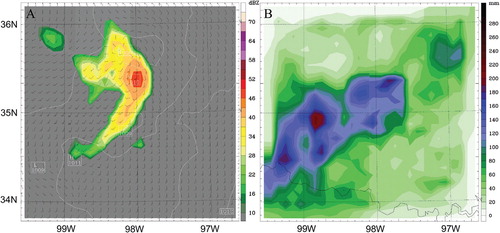
4.1.3. Radar reflectivity.

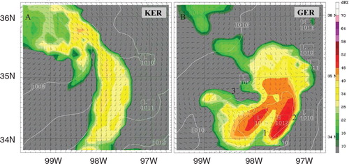
The simulated radar reflectivity with KER and GER (Fig. 5) clearly underlines the sensitivity to the CPS. KER estimates a lower radar reflectivity (37–40 dBZ) compared to GER (52–55 dBZ), which is close to the observations (Fig. 1). The convective system in GER reflects more characteristics of a typical mesoscale convective system with pressure transients – a mesohigh (1), pre-squall low (2) and wake low (3) than a tropical cyclone.

Fig. 5.  Simulated radar images and sea level pressure of (A) KER and (B) GER of domain 2 on 19 August 2007, 12:30 UTC.

4.2. Analysis of experiment 1

To understand and interpret the model results in depth, we studied the significant levels for convection from 18 to 19 August 2007 for grid point (x, y)=(18,10), that is, (34.50 N, 97.90 E) in Fig. 6. This point was selected because in most runs the maximum precipitation occurred at this point. Note that these values are, contrary to Figs. 3 and 4, from a fixed point and therefore a direct comparison with these figures is not possible. Within the modelled time series, one can distinguish between two regimes in model behaviour. First, the sensitivity is largest to the PBL-schemes (from 14:00 to 21:00 UTC), whereas later on the CPS's are responsible for the largest differences. In part I, the runs using ETA reach CAPE up to 1.2×10³ J kg⁻¹, whereas the MRF runs provide CAPE values of 0.2×10³−0.4×10³ J kg⁻¹ (Fig. 6a). The same occurs in Fig. 6b, where the ETA runs are very moist (high T _d ) and the MRF runs are dryer (low T _d ). The LCL of all MRF runs is higher than for ETA (Fig. 6c). The smaller CAPE, lower T _d and higher LCL all point towards a deeper PBL in MRF, which can be explained by the enhanced mixing in the MRF scheme because of the counter gradient terms. These results agree with the findings from Braun and Tao (2000) and Steeneveld et al. (2008).

Fig. 6.  Modeled CAPE (A) and dew point temperature (B) at 2 meters for all eight runs. Figure B has same legend as A. Figure C and D show the LCL and LFC of respectively the runs with KF2 and the runs with Grell. Shown figures indicate August 18–19, 2007, with time in UTC.

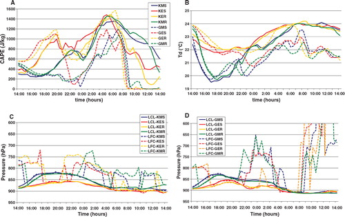
Part II starts around 22:00 UTC, when the clustering between the PBL schemes slowly transforms into a division between the convection schemes (Fig. 6b). Around 8:00 UTC, CAPE and T _d show a clear drop, especially with Grell, indicating that Erin has arrived and that deep convection is triggered. The CAPE and T _d (Fig. 6a and b) decrease substantially with Grell than with KF2, indicating that the convection is much stronger in Grell than in KF2. This is also visible in Fig. 6c, where in the LCL of the KF2 runs there is a difference between ETA and MRF, but in the Grell runs all four LCL's are the same, indicating that the influence of the CPS is dominant over the other processes. These results show that the PBL processes have a large influence on the timing (e.g. point ‘A’ in Fig. 2) and intensity of convection (e.g. point ‘B’ in Fig. 2), but once convection really starts, the convective processes are dominant over the other processes (Fig. 6c).

Conversely, it should be noted that the forecasted PBL is also influenced by the downdraft formulation in the convection scheme. The stronger the effect of the downdraft formulation, the more efficiently the dry and cold air is brought into the PBL. In our study, the Grell downdraft formulation is more efficient than for KF2, which explains the lower T _d . In the following sections, we discuss how KF1 produces a stronger DMF than KF2 (Section 4.4, Fig. 10a).

Fig. 10.  (A) Modelled updraft and downdraft maximum of KER (KF2) and KER1 (KF1) during the period 18–19 August 2007. (B) Modelled updraft and downdraft maximum of DDFORM and RHDSL during the period 18–19 August 2007. A simulation time of 48 hours corresponds to 19 August 2007, 00:00 UTC. Note the different range on the y-axis of panels A and B.

Overall, the sensitivity to microphysics is relatively small in our simulations. However, in general, microphysical processes have shown to be very important in cyclone modelling, particularly over sea (McFarquhar et al., 2006; Pattnaik and Krishnamurti, 2007). Though, in reality TS Erin had cyclone characteristics, these were less pronounced in the model simulations. More precisely, especially the runs with Grell much more resemble a typical MCS than a tropical cyclone (Section 4.1.3). The sensitivity of a MCS to microphysics is limited because they are largely dominated by macrophysics rather than microphysics (Moncrieff and Liu, 2006).

MM5 model output appears to be very sensitive to the selected PBL scheme. This corresponds to the findings by Braun and Tao (2000) and Steeneveld et al. (2008). Hence, we underline their conclusions, which are mainly caused by the different descriptions of vertical mixing. The countergradient terms incorporated in the MRF scheme enhances mixing, which results in a drier and higher PBL and reduces the potential for deep convection.

Although it is known that NWP is sensitive to the selected CPS, sensitivity as large as here was not a priori expected. Hence, it will be useful to examine in detail as to why KF2 largely underestimates the re-intensification of TS Erin. Basically, KF2 differs from KF1 in three aspects: CAPE estimation (diluted or undiluted), the presence of a minimum entrainment rate (in KF1 but not in KF2) and the downdraft formulation. Consequently, it is tempting to examine the performance of KF1 on the re-intensification of TS Erin.

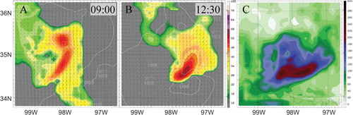
When using KF1 instead of KF2, both the simulated radar reflectivity and the total precipitation differ substantially from KER (Fig. 7). Accumulated precipitation is much higher (Fig. 6c), and the spatial distribution of the radar reflectivity at 09:00 (Fig. 7a) is much closer to the observations with KF1 than with KF2 (as in Figs. 2 and 5a). Despite the promising radar images at 09:00 UTC, at 12:30 UTC (Fig. 7b) the system shifted course and moved southeast, which is not consistent with observations. Also, the radar reflectivity loses TC characteristics and starts resembling a MCS (like GER). Consequently, the question as to which of the differences in model formulation between KF1 and KF2 is decisive for the final model outcome arises. To answer this question, a second set of experiments were performed.

Fig. 7.  Modelled radar reflectivity for KF1-ETA-Reisner Graupel on 19 August 2007, 09:00 UTC (A) and 12:30 UTC (B) and cumulative precipitation (C) from the complete simulation time, all from domain 2.

4.3. Results of experiment 2

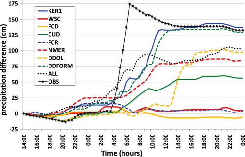
To understand the physical background of the differences in model behaviour between KF1 and KF2, we performed a number of sensitivity tests to diagnose its origin. Table 2 lists the performed permutations to the KF2 scheme and Section 3.2.3 describes the different modifications, which were returned to its original state (as in KF1) for these sensitivity tests. The modifications affect the accumulated precipitation differently (Fig. 8). Note that the reported values are again the accumulated maximum values per time step over domain 2, relative to run KER as a reference. It is evident that the sensitivity to the shallow convection modus (WSC), the fixed cloud radius (FCR) and the fixed cloud depth (FCD) is evidently limited, compared to the other modifications. When CAPE is based on an undiluted parcel instead of a diluted parcel (CUD), accumulated precipitation increases by ~50 mm. This is however insufficient to reach the accumulated precipitation as in KER1. By removing no minimum entrainment rate (NMER) and modifying the DDOL, maximum cumulative precipitation increases by ~80 and ~100 mm, respectively. Finally, the modified downdraft formulation (DDFORM), including the downdraft closure assumption enhances the cumulative precipitation by ~125 mm. Because the downdraft formulation also influences the propagation of convection (Knupp, 1987), a closer look at the spatial precipitation distribution is needed (Fig. 9a). The cumulative precipitation of the complete simulation of the five runs is substantially different from KER (Fig. 2). Fig. 9b shows radar reflectivity of the same five runs on the peak intensity of Erin during the simulation. Comparing CUD with KER, one finds an increase in precipitation but no real shift in spatial distribution. The radar image of CUD shows slightly higher radar reflectivity but, in general, differences with the reference run are modest.

Fig. 8.  Modelled cumulative precipitation for runs 9–17 (Table 2) with the reference run (run 3 – KER) subtracted, from 18 August 2007, 14:00 UTC till 19 August 2007, 24:00 UTC.

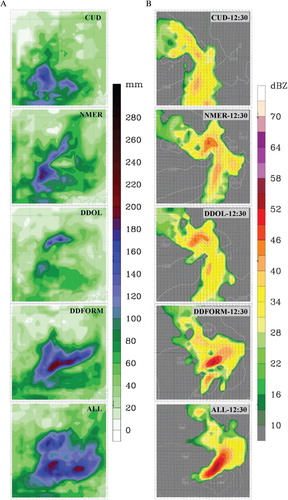
Fig. 9.  (A) Modelled cumulative precipitation of the complete simulation with different permutations for the convection scheme. (B) Simulated radar reflectivity on 19 August 2007, with time in UTC. Different permutations within the convection scheme are shown.

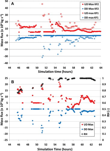
Table 2. Experimental set-up for experiment 2

	Run	CPS	Mod nr.	Modification (same as in KF1)
9	KER1	KF1	–	–
10	NSC	KF2	1	No shallow convection
11	FCD	KF2	2	Fixed cloud depth (3 km)
12	CUD	KF2	3	Cape undiluted
13	FCR	KF2	4	Fixed cloud radius (1500 meter)
14	NMER	KF2	5	No minimum entrainment rate
15	DDOL	KF2	6	Downdraft origination level
16	DDFORM	KF2	7	Downdraft formulation (DDOL as in KF1)
17	ALL	KF2	1–7	All modifications
18	GRELL-DD	GR	8	Downdraft formulation (as in KF2)

Run NMER differed from KER (Fig. 9a), both in maximum values as well as spatial distribution. The most distinct difference was the band of heavy precipitation that had extended to the northeast compared to reference run KER. The modelled radar reflectivity also corresponded very well with observations (Fig. 1), although it still underestimated the intensity of convection. NMER is the only simulation that showed an eye-like feature and an associated closed circulation, as was observed. The DDOL run reproduced to a large extent a similar spatial distribution as KER, although an additional band of precipitation appeared northeast of the original location of maximum precipitation. The radar reflectivity was higher than in KER, and it showed spatial characteristics of a cyclone, but it lacked the eye-like feature with a closed circulation. The DDFORM run showed a spatial characteristic in the accumulated precipitation very similar to that of KER1 (KF1) in Fig. 7c. The enhanced precipitation was distributed over a much wider area than with KER, which indicated that this modification had the largest effect of all suggested permutations, on both the spatial distribution and cumulative precipitation. Also, radar reflectivity was much higher compared to KER (49–52 dBZ instead of 37–40 dBZ). The run ALL (KF2 with all the modifications) showed, as expected, high resemblance with run KER1 (KF1). As there are still some minor differences in the code between KER1 and ALL, the results were not exactly the same.

4.4. Analysis of experiment 2

From the previous section it is obvious that apparently small differences in scheme formulation can result in very different results. To understand the physical background of the model behaviour, this section analyses the results in depth. CAPE estimates based on undiluted parcels are higher than for diluted parcels. Since CAPE is part of the closure assumptions, modifications result in higher mass fluxes and therefore higher precipitation, which can enhance mass fluxes up to a factor ~6 (Kain, 2004). Larger downdraft mass fluxes can also trigger more convection, creating more widespread convection, as seen in the CUD run by the extra band of precipitation east of the highest peak in precipitation (Fig. 9a).

Removing a minimum entrainment rate in the cloud model reduces, under some circumstances, the entrainment of the updraft with environmental air and therefore enhances the mass fluxes. Vertical cross sections reveal that during the peak intensity of Erin, NMER has a cloud base of 950 hPa and KER a cloud base of 800 hPa (not shown). With the reduced entrainment, the altered KF2 scheme finds the USL at lower altitude, with deep enough clouds to initiate convection. This affects the convection intensity, and less precipitation is evaporated between cloud base and the surface. A striking feature of NMER is the closed circulation with an eye-like feature. The enhanced mass fluxes, that is, enhanced convection, can lead to a spin-up of vorticity in Erin's centre and produce cyclone features (Bister and Emanuel, 1997).

Having DDOL defined at the lowest θ_es (as in KF1) results in a higher and more variable DDOL than with a fixed height above the USL (as in KF2). A higher DDOL produces more ‘tall and skinny’ downdrafts; a lower origination level gives more ‘short and fat’ downdrafts (Kain, 2004). One would expect that a ‘tall and skinny’ downdraft, which gives less downdraft outflow in the sub-cloud layer thus less propagation of convection, would result in less precipitation. Surprisingly, the opposite is found in Fig. 9a (DDOL). Within a specific region, the precipitation increases with more than 100 mm with respect to KER. When examining the DDOL, it indeed varies from 780 to 300 hPa (not shown). The reason behind the enhanced precipitation in the DDOL run will be discussed later.

The influence of the different downdraft formulation (DDFORM) is hard to predict a priori because many variables are involved in the calculation for both the KF1 and KF2 formulation. A clear physical interpretation from Fig. 8 is therefore, both for DDOL and DDFORM, not possible and a further in-depth look at the downdraft properties is necessary. Hence, we study the modelled down- and updraft maxima for both the KER and KER1 (Fig. 10a). The values have been taken at the point of maximum cumulative precipitation for each run from domain 2. The difference between both runs is evident, namely, the UMF of KER1 is almost always larger, but especially the DMF of KER1 is much larger than in KER. Overall, the ratio DMFFRC within the time interval (t=44–64, that is, 18 August, 20:00 UTC, till 19 August, 20:00 UTC) is 0.05 for KER and 0.5 for KER1. This indicates that the KF2 scheme hardly produces any downdrafts. For a closer look, we consider the equation in KF2, as described in Section 3.2.3.

Evidently, the RH_DSL strongly influenced the DMF magnitude. The RH_DSL during Erin's re-intensification varied between 0.97 and 1, which gave very small downdrafts, if at all. To examine whether the downdraft formulation within KF1 produced any downdrafts with a high RH, we examined the DDFORM run in more detail. Even with RH close to 1, the DMFFRC was still very high (Fig. 10b). For example, at t=55 h (19 August 07:00 UTC) the DMFFRC amounted to 0.83, with a RH of 0.98. Using the KF2 downdraft formulation resulted in a DMFFRC of 0.038. This is because in KF1 the determining variables in downdraft strength are cloud base height and PE, where the latter is related to the vertical wind shear. Therefore, in cases with a high RH_DSL and large vertical wind shear, KF2 will produce very small downdrafts, or none at all, and KF1 will produce very large downdrafts, because of its dependence on vertical wind shear.

Subsequently, the question as to which parameterisation is closest to physical reality arises. Numerous studies have shown that the parameterisation of moist downdrafts is crucial for reproducing many of the mesoscale characteristics within convective clouds (e.g. Wang and Seamon, 1997). Consensus exists that downdraft simulation is a very important CPS aspect, but how this downdraft should be formulated is still under debate (e.g. Ferrier et al., 1996; Kain, 2004). Kain (2004) modified the downdraft formulation such that it became RH dependent because the original dependence on wind shear and cloud base height lacked robust physical foundation. However, is it physically correct that the KF2 scheme produced hardly or no downdrafts at all during Erin's re-intensification? To answer this question, a further in-depth look at tropical cyclogenesis is necessary. Bister and Emanuel (1997) describe the evolution of a tropical cyclone from a pre-existing MCS (approximately comparable to remnants of TS Erin). First, the upper part of the lower troposphere is cooled and moistened by evaporation of high stratiform precipitation. This results in a cold-core vortex in the lower troposphere and an upper tropospheric warm-core vortex because of anvil heating. Second, as the system evolves further, the cold-core vortex descends into the boundary layer and favours redevelopment of convection in two ways. On one hand, the vortex winds enhance (sea) surface fluxes, and on the other hand the cold core aloft reduces the boundary layer θ_e needed for convection. The redeveloping convection further increases vorticity near the surface, resulting in higher wind speeds. The high RH because of the evaporation of stratiform precipitation diminishes evaporation of rain, which is the main source for the DMF, and thus discourages the convective downdrafts. These downdrafts would bring air with low θ_e into the PBL, preventing further convection and decreasing positive vorticity. When we analyse the environment and location of Erin's intensification prior to arrival, indeed stratiform precipitation is simulated and mid-level humidity increases because of evaporation of rain (not shown). As a consequence, the KF2 downdraft formulation hardly generates downdraft because of the high RH. The relatively strong downdrafts with the KF1 scheme, even with a very high RH, prevent tropical cyclogenesis.

To further verify the hypothesis that the downdraft dependence on PE and vertical wind shear causes the KF1 scheme to simulate a MCS instead of a tropical cyclone, we have modified the downdraft formulation in the Grell scheme to be the same as in KF2. We have done this by removing the wind shear dependency and implementing the, RH-dependent, KF2 downdraft closure (see Section 3.2.3 for a description), referred to as Grell-DD. In this way, we can learn whether the relatively high sensitivity to the downdraft formulation is limited to the KF schemes, or whether it also applies to other mass-flux convection schemes. Fig. 11 shows the total cumulative precipitation and the radar reflectivity of Grell-DD. The trajectory of the modelled system has changed to more northeasterly direction, and the excessive precipitation has disappeared. Although, Grell-DD slightly underestimates the precipitation and the radar reflectivity, the overall picture shows much better resemblance to observations. These results show that the sensitivity to downdraft formulation is not limited to KF but also applies to Grell and most likely other CPS's and weather models.

Fig. 11.  Simulated radar reflectivity (A) on 19 August 2007, 13:00 UTC and total cumulative precipitation (B) from domain 2 of run 19 (Grell-DD).

Overall, it is clear that the downdraft formulation has a very large influence on the different simulations. The downdraft formulations of KF1 and Grell are not well suited for the simulation of TCs in a sheared environment because they both use wind shear and cloud height (KF1) as determining factors in their downdraft strength, whereas with tropical cyclogenesis the RH is the determining factor in the downdraft strength. Subsequently, both with KF1 and Grell, the high DMF's result in a system with completely different dynamics (MCS, Squall line) resulting also in a different trajectory (too far south). In general, every situation with high/low vertical wind shear combined with high/low RH_DSL will result in a high sensitivity to the downdraft formulation within the convection scheme. The unmodified KF2 scheme severely underestimates the precipitation and radar reflectivity but shows the best resemblance on surface wind speeds. When no minimum entrainment rate is added to the scheme, more convection is generated resulting in a system, which has more features of a tropical cyclone and, overall, shows best resemblance with observations. Hence, KF2 shows the best potential for adequately simulating the re-intensification of TS Erin. The above findings correspond with the results from both Bhaskar and Prasad (2006), where KF2 outperformed Grell and KF1, as also Srinivas et al. (2007), where KF2 outperformed Grell in hurricane simulations.

Finally, we analyse why DDOL results in more precipitation compared to KER (Fig. 10, DDOL). In almost all runs with the KF2 scheme, there are hardly any downdrafts because of the high RH_DSL. Examining RH_DSL on the location of the extra band of precipitation, RH_DSL amounts to 0.8–0.85, whilst in all other runs the RH_DSL is between 0.95–1. When the precipitation in this region falls, the DDOL is located around 300–400 hPa. This gives a DSL of thickness around 500–600 hPa instead of 150 hPa within the original KF2 scheme. The RH decreases higher up in the troposphere, resulting in a lower RH_DSL to determine the DMF. The influence of this DMF is immediately visible in an increase of precipitation of up to 200 mm.

5. Discussion

The large sensitivity to downdraft formulation raises some questions about how PE/DMF (i.e. downdraft closures) should be treated within cumulus schemes. Fritsch and Chappell (1980) were the first ones to introduce PE to the downdraft closure, where they used the strong negative correlation of PE to vertical wind shear found by Marwitz (1972) and Foote and Fankhauser (1973). Grell (1993) and Kain and Fritsch (1993) also implemented this exact formulation despite comprehensive work by Fankhauser (1988), which showed contrasting results compared to Marwitz (1972). Fankhauser suggested: ‘factors controlling thunderstorm precipitation efficiency are more complicated than a simple inverse dependence on vertical wind shear’ and in fact even found a small positive correlation between PE and vertical wind shear. Hence, Fankhauser (1988) stated that further research on this topic was needed. Further work by Ferrier et al. (1996) and Market et al. (2003) emphasised this. Ferrier et al. (1996) evaluated convection schemes that use a functional relationship for calculating PE (vertical wind shear and cloud base height) and found that none of the convection schemes showed consistent agreement with the PE diagnosed from the different 2D simulations. They found that ambient moisture content and the vertical orientation of the updrafts were the main determining parameters in PE. Market et al. (2003) did find a negative correlation between vertical wind shear and PE, contrary to Fankhauser (1988), but the correlation (16.6%) was much smaller than the 87.4% found by Marwitz (1972). They also added convective inhibition and the average RH from surface to LCL as possible determining factors in PE. As a result, Kain (2004) modified the downdraft closure in the KF scheme to a dependency on mid-level RH. Despite the strong evidence brought by Fankhauser (1988), Ferrier et al. (1996) and Market et al. (2003) that PE cannot be described by a simple inverse dependence on vertical wind shear, this formulation is still widely used within cumulus schemes, for example, the SAS scheme and the Grell-Dévényi scheme.

From the review above, and from our results, it appears that the current way downdraft closures are treated in CPS lacks robust physical foundation that covers different environments and, as a consequence, limits the amount of different environments a specific CPS is suitable for. More research on the understanding of the downdrafts processes and the implementation within cumulus schemes is therefore necessary. The recent possibilities to simulate deep convection using large eddy simulation (LES) models (e.g. Böing et al., 2010) can be very promising to the questions raised above. It can help to improve the physical foundation within deep convection schemes as it has done with shallow convection schemes (e.g. de Rooy and Siebesma, 2008), without the need for extensive and expensive measuring campaigns.

6. Conclusions

The re-intensification of TS Erin (2007) over Oklahoma is simulated using the mesoscale model MM5. In addition, a sensitivity analysis to two microphysics, boundary layer and three convection schemes is performed. The unique and explosive re-intensification of Erin is initiated by isentropic lifting of Erin's remnants and positive vorticity advection because of an upper-level short-wave trough passage, combined with a band of warm moist advection at lower atmospheric levels, which favoured tropical cyclogenesis.

MM5 simulations showed surprisingly large sensitivity to the selected physical parameterisation schemes. In particular, the selection of different PBL schemes, MRF and ETA, strongly influenced the model results. Herein, ETA produced more precipitation than MRF. This is explained by the enhanced mixing in MRF, which resulted in a deeper and drier PBL. Consequently, the drier PBL resulted in a relatively small CAPE and therefore less convection was triggered, and if triggered it was less intense.

The largest differences in model results occurred between the convection schemes KF1, KF2 and Grell. Both KF1 and Grell generated most precipitation, with KF1 being closest to the observations. Unfortunately, both schemes produced precipitation too far south and failed to reproduce the re-intensification to a TS with its typical eye-like structure and strong surface winds.

The reason behind this deficiency is that the simulated downdraft is calculated based on the wind shear (both Grell and KF1) and cloud base height (only KF1), which allow for very strong downdrafts in completely saturated environments. This is inconsistent with downdraft physics that suggests that downdrafts diminish with a high RH within the DSL (Bister and Emanuel, 1997). The strong downdrafts alter the system's dynamics and re-intensify the system to a MCS or a squall line. This is explained by the downdraft outflow, which interacts with the LLJ from the southeast, creating a convergence zone to the southeast of TS Erin, which consequently triggers more convection, resulting in a different trajectory (east instead of northeast) and system dynamics. When the Grell scheme is modified, with the simulated downdraft made RH dependent (as in KF2), the trajectory and radar reflectivity match better with observations. The KF2 scheme underestimates precipitation but better simulates the wind maxima and trajectory.

When the KF2 scheme is modified by removing the minimum entrainment rate, convection increases and the simulation closely resembles the observations, with an eye-like structure and a closed circulation. Overall, this simulation is closest to observations. Implementing the KF1 downdraft formulation (wind shear dependent) in KF2 stimulated convection and precipitation, but again intensified to a MCS with the maximum precipitation too far south. Overall, the results can be divided into two groups. One with downdraft dependency on vertical shear, which produced a MCS/squall line with heavy precipitation too far south, and one with downdraft dependency on RH, which gave best resemblance to observations concerning radar images and track, but with insufficient convection. Hence, we conclude that the model is extremely sensitive to the downdraft formulation for this case, and that KF2 shows the best potential in adequately simulating the re-intensification of TS Erin.

These results stress the need for a better physical foundation for the parameters and assumptions used in deep convection schemes. Especially, the functional relationship for PE in Grell needs more attention because the current formulation can give the unphysical result of very strong downdrafts in completely saturated environments. Hence, more research is needed on how to treat downdraft closures and, if used in the downdraft formulation, functional relationships for PE.

Acknowledgements

The authors are grateful to Bert Holtslag, Kees van den Dries, Jordi Vila, G.A. Grell and Jeremy Pal. Oklahoma Mesonet data are provided courtesy of the Oklahoma Mesonet, ‘a cooperative venture between Oklahoma State University and The University of Oklahoma and supported by the taxpayers of Oklahoma’. Moreover we thank wunderground.com for Fig. 1. Finally, the authors acknowledge two anonymous reviewers for their constructive comments and suggestions.

References

- Arndt, D. S, Basara, J. B, McPherson, R. A, Illston, B. G, McManus, G. D and co-author. 2009. Observations of the overland reintensification of tropical storm Erin (2007). Bull. Amer. Meteor. Soc. 90, 1079–1093. 10.3402/tellusa.v64i0.17417.
- Bhaskar R. D. V. Prasad D. H. Numerical prediction of the Orissa super-cyclone (1999): sensitivity to the parameterization of convection, boundary layer and explicit moisture processes. Mausam. 2006; 57: 61–78.
- Bister M. Emanuel K. A. The genesis of hurricane Guillermo: TEXMEX analyses and a modeling study. Mon. Wea. Rev. 1997; 125: 2662–2682.
- Böing, S. J, Jonker, H. J. J, Siebesma, A. P and Grabowski, W. W. 2010. Influence of subcloud-layer structures on the transition to deep convection. 19th Symposium on Boundary-Layers and Turbulence, Keystone, CO, USA, 2–6 August2010.
- Bosart L. F. Bartlo J. A. Tropical storm formation in a baroclinic environment. Mon. Wea. Rev. 1991; 119: 1979–2013.
- Braun S. A. Tao W. K. Sensitivity of high-resolution simulations of hurricane Bob (1991) to planetary boundary layer parameterizations. Mon. Wea. Rev. 2000; 128: 3941–3961.
- Brennan M. J. Knabb R. D. Mainelli M. Kimberlain T. B. Atlantic hurricane season of 2007. Mon. Wea. Rev. 2009; 137: 4061–4088. 10.3402/tellusa.v64i0.17417.
- Brock, F. V, Crawford, K. C, Elliott, R. L, Cuperus, G. W, Stadler, S. J and co-authors. 1995. The Oklahoma Mesonet: a technical overview. J. Atmos. Ocean. Tech. 12, 5–19.
- Chien F. C. Jou B. J. D. MM5 Ensemble mean precipitation forecasts in the Taiwan area for three early summer convective (Mei-Yu) seasons. Wea. Forecasting. 2004; 19: 735–750.
- Cuxart, J, Holtslag, A. A. M, Beare, R. J, Bazile, E, Beljaars, A and co-authors. 2006. Single-column model intercomparison for a stably stratified atmospheric boundary layer. Bound-Layer Meteor. 118, 273–303. 10.3402/tellusa.v64i0.17417.
- Dudhia J. Numerical study of convection observed during the Winter Monsoon Experiment using a mesoscale two-dimensional model. 1989; 46: 3077–3107.
- Dudhia J. A nonhydrostatic version of the Penn State–NCAR mesoscale model: validation tests and simulation of an Atlantic cyclone and cold front. J. Atmos. Sci. 1993; 121: 1493–1513.
- Emanuel K. A. Environmental factors affecting tropical cyclone power dissipation. Mon. Wea. Rev. 2007; 20: 5497–5509. 10.3402/tellusa.v64i0.17417.
- Evans J. L. Hart R. E. Objective indicators of the life cycle evolution of extratropical transition for Atlantic tropical cyclones. J. Climate. 2003; 131: 909–925.
- Fankhauser J. C. Estimates of thunderstorm precipitation efficiency from field measurements in CCOPE. Mon. Wea. Rev. 1988; 116: 663–684.
- Ferrier B. S. Simpson J. Tao W.-K. Factors responsible for precipitation efficiencies in midlatitude and tropical squall simulations. Mon. Wea. Rev. 1996; 124: 2100–2125.
- Foote G. B. Fankhauser J. C. Airflow and moisture budget beneath a north–east Colorado hailstorm. Mon. Wea. Rev. 1973; 12: 1330–1353.
- Fritsch J. M. Chappell C. F. Numerical prediction of convectively driven mesoscale pressure systems. Part I: convective parameterization. J. Appl. Meteor. 1980; 37: 1722–1733.
- Grell G. A. Prognostic evaluation of assumptions used by cumulus parameterization. J. Atmos. Sci. 1993; 121: 764–787.
- Grell, G. A, Dudhia, J and Stauffer, D. R. 1995. A Description of the Fifth-generation Penn State/NCAR Mesoscale Model (MM5). NCAR Tech. Note TN-398+STR, 122 pp.
- Holtslag A. A. M. Boville B. Local versus nonlocal boundary-layer diffusion in a global climate model. 1993; 6: 1825–1842.
- Hong S. Y. Pan H. L. Nonlocal boundary layer vertical diffusion in a Medium-Range Forecast model. J. Climate. 1996; 124: 2332–2339.
- Janjić Z. I. The step-mountain Eta coordinate model: further developments of the convection, viscous sublayer, and turbulence closure schemes. Mon. Wea. Rev. 1994; 122: 927–945.
- Kain J. S. The Kain-Fritsch convective parameterization: an update. Mon. Wea. Rev. 2004; 43: 170–181.
- Kain, J. S and Fritsch, J. K. 1993. Convective parameterization for mesoscale models: the Kain-Fritsch scheme. J. Appl. Meteor. No. 46, Amer. Meteor. Soc., 165–177.
- Knabb, R. D. 2008. Tropical Cyclone Report: Tropical Storm Erin. Online at: http://www.nhc.noaa.gov/pdf/TCR-AL052007_Erin.pdf.
- Knupp K. R. Downdrafts within high plains cumulonimbi. Part I: general kinematic structure. 1987; 44: 987–1008.
- Knupp K. R. Cotton W. R. Convective cloud downdraft structure: An interpretive survey. 1985; 23: 183–215. 10.3402/tellusa.v64i0.17417.
- Kong, K and Gedzelman, S. 2004. MM5 Simulations of sub-tropical storm Allison over southern Mississippi Valley. 26th Conf. Hurricanes and Tropical Meteor. Amer. Meteor. Soc. Boston, 2–7 May 2004, Miami, Florida, USA, paper 13C4.
- Liang X. Z. Xu M. Kunkel K. E. Grell G. A. Kain J. S. Regional climate model simulation of U.S.–Mexico summer precipitation using the optimal ensemble of two cumulus parameterizations. 2007; 20: 5201–5207. 10.3402/tellusa.v64i0.17417.
- Liu C. Moncrieff M. W. Sensitivity of cloud-resolving simulations of warm-season convection to cloud microphysics parameterizations. 2007; 135: 2854–2868. 10.3402/tellusa.v64i0.17417.
- Market P. S. Allen S. N. Scofield R. Kuligowski R. Gruber A. Precipitation efficiency of warm-season Midwestern mesoscale convective systems. J. Climate. 2003; 18: 1273–1285.
- Marwitz J. D. Precipitation efficiency of thunderstorms on the High Plains. Mon. Wea. Rev. 1972; 6: 367–370.
- McFarquhar, G. M, Zhang, H, Heymsfield, G, Halverson, J. B.,Hood, R and co-authors. 2006. Factors affecting the evolution of hurricane Erin (2001) and the distributions of hydrometeors: role of microphysical processes. 63, 127–150. 10.3402/tellusa.v64i0.17417.
- McPherson R. A, Fiebrich, C. A, Crawford, K. C, Elliott, R. L, Kilby, J. R and co-authors. 2007. Statewide monitoring of the mesoscale environment: a technical update on the Oklahoma Mesonet. Wea. Forecasting. 24, 301–321. 10.3402/tellusa.v64i0.17417.
- Mellor, G. L and Yamada, T. 1974. A hierarchy of turbulence closure models for planetary boundary layers. J. Res. Atmos. 31, 1791–1806. DOI: http://dx.doi.org/10.1175/1520-0469(1974)031<1791:AHOTCM>2.0.CO;2.
- Moncrieff M. W. Liu C.-H. Representing convective organization in prediction models by a hybrid strategy. J. Atmos. Sci. 2006; 63: 3404–3420. 10.3402/tellusa.v64i0.17417.
- Monteverdi, J. P and Edwards, R. 2008. Documentation of the overland reintensification of Tropical Storm Erin over Oklahoma. August18, 2007. Preprints, In: 24th Conf. on Severe Local Storms. Savannah, GA, Amer. Meteor. Soc., P4.6.
- Pattnaik S. Krishnamurti T. N. Impact of cloud microphysical processes on hurricane intensity, part 2: sensitivity experiments. J. Atmos. Sci. 2007; 97: 127–147. 10.3402/tellusa.v64i0.17417.
- Rao D. V. B. Prasad D. H. Sensitivity of tropical cyclone intensification to boundary layer and convective processes. J. Atmos. Sci. 2007; 41: 429–445. 10.3402/tellusa.v64i0.17417.
- Reisner J. Rasmussen R. M. Bruintjes R. T. Explicit forecasting of supercooled liquid water in winter storms using the MM5 mesoscale model. 1998; 124: 1071–1107. 10.3402/tellusa.v64i0.17417.
- Rio, C, Hourdin, F, Grandpeix, J. Y and Lafore, J. P. 2009. Shifting the diurnal cycle of parameterized deep convection over land. Meteor. Atmos. Phys. 36, L07809. DOI: 10.3402/tellusa.v64i0.17417.
- de Rooy W. C. Siebesma A. P. A simple parameterization for detrainment in shallow cumulus. Nat. Hazards. 2008; 136(2): 560–576. 10.3402/tellusa.v64i0.17417.
- Srinivas C. V. Venkatesan R. Bhaskar Rao D. V. Prasad D. H. Numerical simulation of Andhra severe cyclone (2003): model sensitivity to the boundary layer and convection parameterization. Quart. J. Roy. Meteor. Soc. 2007; 164: 1465–1487. 10.3402/tellusa.v64i0.17417.
- Steeneveld, G. J, Mauritsen, T, de Bruijn, E. I. F, Vilà-Guerau de Arellano, J, Svensson, G and co-author. 2008. Evaluation of limited-area models for the representation of the diurnal cycle and contrasting nights in CASES-99. Geophys. Res. Lett. 47, 869–887. 10.3402/tellusa.v64i0.17417.
- Stensrud, D. J. 2007. Parameterization Schemes: Keys to Understanding Numerical Weather Prediction Models. Cambridge University Press: Cambridge, 459. pp.
- Troen I. B. Mahrt L. A simple model of the atmospheric boundary layer: sensitivity to surface evaporation. Pure Appl. Geophys. 1986; 37: 129–148. 10.3402/tellusa.v64i0.17417.
- Wang W. Seaman N. L. A comparison study of convective parameterization schemes in a mesoscale model. J. Appl. Meteor. Climatol. 1997; 125: 252–278.
- Wisse J. S. P. Vilà-Guerau de Arellano J. Analysis of the role of the planetary boundary layer schemes during a severe convective storm. 2004; 22: 1861–1874. 10.3402/tellusa.v64i0.17417.
- Zhang D-L. Fritsch J. M. Numerical simulation of the meso-β scale structure and evolution of the 1977 Johnstown flood. Part I: Model description and verification. Bound-Layer Meteorol. 1986; 43: 1913–1943.