Wind gust estimation for Mid-European winter storms: towards a probabilistic view

Abstract

Three wind gust estimation (WGE) methods implemented in the numerical weather prediction (NWP) model COSMO-CLM are evaluated with respect to their forecast quality using skill scores. Two methods estimate gusts locally from mean wind speed and the turbulence state of the atmosphere, while the third one considers the mixing-down of high momentum within the planetary boundary layer (WGE Brasseur). One hundred and fifty-eight windstorms from the last four decades are simulated and results are compared with gust observations at 37 stations in Germany. Skill scores reveal that the local WGE methods show an overall better behaviour, whilst WGE Brasseur performs less well except for mountain regions. The here introduced WGE turbulent kinetic energy (TKE) permits a probabilistic interpretation using statistical characteristics of gusts at observational sites for an assessment of uncertainty. The WGE TKE formulation has the advantage of a ‘native’ interpretation of wind gusts as result of local appearance of TKE. The inclusion of a probabilistic WGE TKE approach in NWP models has, thus, several advantages over other methods, as it has the potential for an estimation of uncertainties of gusts at observational sites.

• windstorm
• wind gust estimation
• TKE
• COSMO-CLM
• probabilistic approach

1. Introduction

Wind gusts associated with windstorms are one of the main sources of economic and insured losses over Europe. For example, storm Kyrill (18 January 2007) caused insured losses of about €2.4 billion in Germany alone and caused a widespread disruption of normal social activities, public transportation and energy supply, as well as a large number of fatalities over large parts of Europe (cf. Fink et al., 2009). Therefore, the correct estimation and forecast of wind gusts associated with winter storms may enhance the capability of issuing accurate severe weather warnings and is of great value in scientific, societal and economical terms. Several studies on the estimation of gusts associated with the passage of windstorms were recently undertaken either using mesoscale modelling or statistical approaches (e.g. Brasseur, 2001; Goyette et al., 2003; De Rooy and Kok, 2004; Agustsson and Olafsson, 2004, 2009; Friederichs et al., 2009; Pinto et al., 2009). One of the recent applications is to estimate potential losses associated with wind gusts (e.g. Della-Marta et al., 2009, 2010; Pinto et al., 2010; Schwierz et al., 2010). In these studies, very different approaches for wind gust estimation (WGE) are used. From this fact, the following questions arise: Which complexity of a WGE approach is necessary to obtain good WGEs? Which numerical weather prediction (NWP) model information may be provided that contributes to a WGE? Is a simple and self-suggesting approach based on the definition of subscale kinetic energy able to consider the obvious stochastic nature of gusts, and how does it compare to standard WGE methods?

Simulated near-surface winds from NWP models are usually smaller than observed wind gusts. This fact is related to (1) the formulation of model variables as averages over a space and time (grid box and time step) and (2) the high temporal variability of gustiness, especially during strong wind episodes. From the observational point of view, gust parameterisation reduces to the problem how a probability distribution of highly resolved wind speeds changes when the according time series is averaged. For NWP applications, model-resolved variables like wind speed and measures for the state of turbulence can be used to estimate gusts. In general, three techniques have been established: (1) the use of a gust factor as fraction between gust and mean wind speed (based on the original work of Durst, 1960; e.g. Wieringa, 1973; Verkaik, 2000), varying with atmospheric stability and/or roughness length in the environment; (2) the interpretation of gusts as downwards-transition of higher level boundary-layer momentum (e.g. Brasseur, 2001; Brasseur et al., 2002) and (3) the understanding of gusts as mean wind plus a part connected with turbulent kinetic energy (TKE). If TKE is not available, wind drag in terms of friction velocity (e.g. Schulz and Heise, 2003), atmospheric stability indices and wind direction, describing the advection of TKE from near-by regions with different roughness characteristics (Agustsson and Olafsson, 2004), can be used as a proxy for the turbulence state.

Wind gusts are affected by particular characteristics of the model topography, mainly land cover (in terms of roughness) and surface elevations, which induce turbulent eddies and, thus, influence the turbulence state of the atmosphere. The WGE formulation has to consider this subscale influence; its quality depends on the calibration of turbulence-related WGE parameters. One major setback is that spatially distributed observations usually do not provide sufficient information about the atmospheric turbulence; a statistical calibration of the turbulence-related part of a WGE is not possible. From the viewpoint of atmospheric modelling, wind gusts show a stochastic behaviour. Thus, rather than predicting absolute values, the estimation of a range of probability at which a gust value may occur appears to be an appropriate and skilful information. Further, such a probability range is also very helpful for various applications, for example, when deciding whether issuing severe weather warnings (e.g. Wichers Schreur and Geertsema, 2008).

In the following sections, a basic formulation of a turbulence-driven WGE method, hereafter called WGE TKE, considering a probabilistic extension, is described. Results of two standard WGE methods considering the turbulence state of the atmosphere locally and non-locally are compared with this new WGE method. The two standard WGE methods are the German Weather Service (DWD; Deutscher Wetterdienst) approach in COSMO-CLM, which uses friction velocity as predictor for turbulence (Schulz and Heise, 2003; Schulz, 2008), and the approach of Brasseur (2001), which estimates gusts considering a possible downward transition of air from higher atmospheric levels, carrying high momentum. The new WGE TKE approach defines the maximum available kinetic energy by interpreting TKE in a statistical sense as measure for wind speed variance. The probabilistic extension assesses the probability range of local gust factors statistically from observations. The forecast capability of the methods is tested by computation of proper skill scores. For the evaluation of WGE methods, a set of historical European windstorms is considered. These were simulated by means of the regional climate model, COSMO-CLM, using reanalysis data as boundary conditions.

This study is organised as follows: Section 2 describes data and the NWP model, while Section 3 presents the different WGE formulations used. The evaluation of WGE methods (Section 4) is divided into four steps: (1) analysis of statistical characteristics of observational data, (2) an overall evaluation of COSMO-CLM simulations, (3) an exemplary comparison of WGE for typical winter storm events and (4) the calculation of skill scores for all events. The discussion of the results is presented in Section 5, and a short summary and conclusion finishes this study (Section 6).

2. NWP model and data

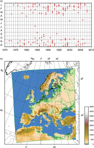
As a basis for this study, model simulations of 158 historical European windstorms between 1972 and 2008 (see Fig. 1a) have been undertaken using the mesoscale atmospheric model, COSMO (http://www.cosmo-model.org). It is mainly designed for application on the meso-β/γ scale using grid resolutions from 20 km down to 1 km. The COSMO model has been widely used for regional climate simulations (e.g. Böhm et al., 2008; Jaeger et al., 2008; Rockel et al., 2008; Lautenschlager et al., 2009; see also COSMO-CLM community at http://www.clm-community.eu).

Fig. 1.  (a) Year and month of simulated storms from 1972 to 2008, in a total of 158 storms and (b) COSMO-CLM model region, including orography, colour scale in m.

In the COSMO model, the non-hydrostatic, fully compressible Navier–Stokes equations are solved on an Arakawa-C grid using a hybrid terrain-following coordinate. In the vertical, the model contains the whole troposphere and parts of the lower stratosphere, the latter mainly as a damping layer. Standard vertical resolutions use 20–45 layers. Physical parameterisations consider an extended version of the level 2.5 scheme after Mellor and Yamada (1982) using prognostic TKE. Cloud microphysics are based on a Kessler-type scheme but contain cloud ice, graupel, and consider advection of cloud water/ice and rain/snow. Radiation effects are estimated using the δ-two-stream approximation (Ritter and Geleyn, 1992). The model has been developed by the DWD and is in operational use for regional NWP in several European weather services. More detailed information may be found in Steppeler et al. (2003).

In this study, COSMO was used in its climate version COSMO-CLM4.0 (Böhm et al., 2008). The most important difference to the NWP version is that no assimilation of observational data and no nudging have been applied. In the vertical, 32 layers in the hybrid pressure-based terrain-following coordinate are used; the horizontal grid consists of 257 × 271 grid boxes with grid sizes of 0.165° resolution on a rotated latitude–longitude grid centred on 8°W, 50.75°N. The thickness of the lowest model layer is approximately 67 m. The first full level, where horizontal momentum and temperature is calculated, is, thus, roughly at 33.5 m above ground. The Runge–Kutta integration scheme with a time step of 90 s and an output interval of 1 h was used. In general, the simulation periods are 96 h, starting 48 h before the peak of the event. For some cases (e.g. Lothar and Martin), the initialisation time had to be slightly changed to guarantee a good representation of that particular storm. The model domain comprises entire Europe and parts of Northern Africa (Fig. 1b). In this study, we focus on Germany for evaluation of the simulations.

In long-term transient COSMO-CLM simulations for Europe (e.g. Böhm et al., 2008; Jaeger et al., 2008), the representation of extreme events like windstorms may differ considerably from the real event. This fact is due to the boundary-only forcing, as atmospheric conditions are mainly inferred over the lateral boundaries. For a more accurate simulation of storms, a shorter model spin-up between initialisation and storm formation is advantageous, as it allows for an evolution of the event closer to the observed development. Therefore, the present set of COSMO-CLM simulations of historical storm events for Germany has been produced. As boundary forcing, ERA40 and ERA-Interim reanalyses (Uppala et al., 2005; Dee et al., 2011) are used. The storms in the overlapping period, 1989–2002, have been simulated using both ERA40 and ERA-Interim in order to assess the influence of the change of boundary forcing. It turned out that storm simulations using either ERA40 or ERA-Interim as atmospheric forcing do not exhibit systematic differences (not shown); hence, they can rather be understood as different realisation of the same storm.

The simulated episodes include all major storms, which affected central Europe between 1972 and 2008. These events were selected based on a storm intensity index, which considers exceedances of the 98th wind speed percentiles and is applied to the reanalysis dataset (Klawa and Ulbrich, 2003; Pinto et al., 2007a; Fink et al., 2009). In this way, the majority of the top-ranking events of the last decades for Germany are collected in the storm list. In addition, a few weaker events known from insurance companies’ reports were included. In order to allow for a comparison with observations, COSMO-CLM output had to be post-processed: In a horizontal plane, the 0.165° gridbox averages were interpolated to locations of the observational sites by means of a distance-weighted interpolation using a Gaussian filter (using 9 × 9 neighbour grid points, and 0.33° lat/lon 1/e-width), including the vertical near-surface wind gradients calculated from model 10 m winds. The vertical gradients are needed for a height correction of winds and gusts: The effect of the vertical displacement dz between surface heights at observational sites and the average model grid box height is considered by adding a correction factor . This kind of first-order correction is absolutely necessary for a comparison between grid box averages of model simulations and local observations.

Wind observations are provided for 37 DWD sites and cover the period from 1950 to 2005 (see Table 1). They consist of hourly wind records from 1979 to 2005, most observations start in 1976 with 3-hourly reports. The data is searched for inhomogeneities; obviously wrong observations are omitted (e.g. 50 m s⁻¹ limited maximum winds). Except for mountain sites, the available number of gust observations typically decreases with distance to the coast: This is due to the fact that in Germany gusts are only reported when they exceed a threshold of 12 m s⁻¹. Such high gust values are less frequent inland.

Table 1. Information on the 37 observational sites, including WMO number, station name, geographical location and height above seal level

WMO no.	Name	Lat (°N)	Lon (°E)	Elevation (m a.s.l.)	Daily hourly data available from		Until	Hourly values	Gusts (%)
10020	SYLT	55.01	8.25	26	1 January 1976	1 January 1979	31 December 2005	226933	20.51
10113	NORDERNEY	53.43	7.09	11	1 January 1976	1 January 1979	31 December 2005	202600	15.44
10129	BREMERHAVEN	53.32	8.35	7	1 January 1976	1 January 1979	31 December 2005	231334	8.77
10147	HAMBURG-FUHLS.	53.38	9.59	11	1 January 1976	1 January 1981	31 December 2005	204360	6.33
10161	BOLTENHAGEN	54.00	11.12	15	1 January 1976	29 August 1977	31 December 2005	230103	11.10
10162	SCHWERIN	53.39	11.23	59	1 January 1976	29 August 1977	31 December 2005	226453	6.27
10170	ROSTOCK-WARNEM.	54.11	12.05	4	1 January 1976	29 August 1977	31 December 2005	229428	9.93
10224	BREMEN	53.03	8.48	5	1 January 1976	1 January 1981	31 December 2005	211507	6.55
10270	NEURUPPIN	52.54	12.49	38	1 July 1975	29 August 1977	31 December 2000	171210	3.73
10291	ANGERMUENDE	53.02	14.00	54	1 July 1975	29 August 1977	31 December 2000	170598	5.27
10317	OSNABRUECK	52.15	8.03	95	1 January 1976	1 January 1979	31 December 2005	177067	6.20
10338	HANNOVER-LANG.	52.28	9.41	59	1 January 1976	1 January 1976	31 December 2005	238068	4.97
10368	WIESENBURG	52.07	12.28	187	11 June 1990	11 June 1990	31 December 2000	88271	10.95
10382	BERLIN-TEGEL	52.34	13.19	36	2 January 1961	2 January 1961	31 December 2000	190182	2.66
10384	BERLIN-TEMP.	52.28	13.24	49	1 January 1950	1 January 1950	31 December 2000	368920	2.11
10385	BERLIN-SCHOEN.	52.23	13.32	45	1 July 1975	29 August 1977	31 December 2000	186349	3.61
10393	LINDENBERG	52.13	14.07	98	1 July 1975	29 August 1977	31 December 2000	182616	3.86
10396	MANSCHNOW	52.33	14.33	12	11 June 1990	11 June 1990	31 December 2000	85474	9.00
10438	KASSEL	51.18	9.27	231	1 January 1976	1 January 1979	31 December 2005	205664	3.03
10453	BROCKEN	51.48	10.37	1142	1 January 1976	29 August 1977	31 December 2005	235536	30.96
10469	LEIPZIG	51.26	12.14	131	1 January 1976	29 August 1977	31 December 2005	229602	5.02
10488	DRESDEN	51.08	13.45	227	1 January 1976	29 August 1977	31 December 2005	223602	5.27
10499	GOERLITZ	51.10	14.57	238	1 January 1976	29 August 1977	31 December 2005	218607	7.75
10513	KOELN-WAHN	50.52	7.10	92	1 January 1976	1 January 1981	31 December 2005	205973	3.16
10609	TRIER-PETRISBERG	49.45	6.40	265	1 January 1976	1 January 1979	31 December 2005	211573	5.71
10637	FRANKFURT/M.	50.03	8.36	112	1 January 1976	1 January 1981	31 December 2005	202463	4.47
10685	HOF-HOHENSAAS	50.19	11.53	567	1 January 1976	1 January 1979	31 December 2005	220504	7.23
10727	KARLSRUHE	49.02	8.22	112	1 January 1976	1 January 1979	31 December 2005	182201	5.87
10729	MANN HElM	49.31	8.33	96	1 January 1976	1 January 1979	31 December 2005	197812	2.55
10738	STUTTGART-ECH.	48.41	9.14	371	1 January 1976	1 January 1981	31 December 2005	181479	3.23
10763	NUERNBERG-KRA.	49.30	11.03	314	1 January 1976	1 January 1981	31 December 2005	194281	2.74
10803	FREIBURGI.BR.	48.00	7.51	269	1 January 1976	1 January 1979	31 December 2005	211339	5.19
10838	ULM	48.23	9.57	571	1 January 1976	1 January 1979	31 December 2005	172506	2.60
10852	AUGSBURG-MUEHLH.	48.26	10.57	462	1 January 1976	1 January 1979	31 December 2005	198728	3.68
10908	FELDBERG/SCHW.	47.53	8.00	1486	1 January 1976	1 January 1979	31 December 2005	211775	24.58
10961	ZUGSPITZE	47.25	10.59	2960	1 January 1976	1 January 1979	31 December 2005	209701	26.26
10980	WENDELSTEIN	47.42	12.01	1832	1 January 1976	1 January 1979	31 December 2005	193686	23.55

In addition, the start/end dates, since/until daily and hourly observations are available. Last two columns mention the amount of available hourly values and the fraction of gusts therein, respectively.

For the evaluation of the RCM simulations, a dataset, including complete life cycles of cyclones obtained from ERA-Interim, is considered. Each track includes information (e.g. core pressure, vorticity) for one cyclone at each time step. The cyclone tracks are computed using an algorithm originally developed by Murray and Simmonds (1991), which is adapted and evaluated for Northern Hemisphere cyclone properties and high-resolution datasets (Pinto et al., 2005; Nissen et al., 2010). Further details on the method, its settings and cyclone climatologies can be found in Murray and Simmonds (1991), Simmonds et al. (1999) and Pinto et al. (2005, 2007b).

3. WGE estimation with different formulations

Wind gust estimation in NWP is a purely diagnostic calculation. The model variables are not influenced by the WGE. A WGE formulation considering model-predicted TKE and a probabilistic estimate of an uncertainty range is introduced here. The TKE approach is based on the relation between mean TKE and gusts , which can be summarised in the relationship:1

or, in a formulation of the gust factor g _v , which is simply the ratio gust/mean wind speed:2

Here, E _max is the maximum kinetic energy, and ɛ _v is the ‘stochastic’ subgrid-scale part of . The random term is related to the difference between actual subscale kinetic energy of the gust and mean TKE and is of stochastic nature for the grid-scale model. It represents the variability of gusts due to the ‘unknown’ portion of small-scale kinetic energy. ɛ _g is not necessarily normally distributed but has obviously an expected value of 0. In this study, stochastic features of ɛ _g are derived from observational data by quantile regression. The model scale parameter used is the ‘average turbulent wind speed’ , which represents the median of the estimated gust distribution. The derivation of eqs. (1) and (2) and quantile regression details are shown in Appendixes A.1 and A.2.

In COSMO-CLM, the standard method for estimating non-convective gusts is to use wind speed interpolated from the lowest model level to 30 m height and the friction velocity u _*:3

The maximum gust v _max is then defined as the maximum occurring in an output time interval, which here is 1 h. The factors 3.0 and 2.4 are motivated by Prandtl-layer theory (Panofsky and Dutton, 1984); the numerical values are determined empirically. A more detailed description and evaluation of this formulation can be found in Schulz and Heise (2003) and Schulz (2008). In general, the friction velocity method and TKE approach are relatively similar, because in both cases a predictor for local turbulence is estimated; in case of WGE DWD, an empirical factor allows for the optimum adaption to observations. In case of WGE TKE, assumptions on the behaviour of the stochastic part ɛ _v have to be made. In this study, the characteristics of ɛ _v are based on gust observations.

Different from these approaches, as it does not consider the local turbulence directly, is the WGE approach named after Brasseur (2001), henceforth referred to as WGE Brasseur. It has been applied in many cases (e.g. Goyette et al., 2003; Pinto et al., 2009) and uses a relation between buoyancy and TKE in order to decide whether a parcel of air may be mixed down from a certain height to the surface, carrying momentum available for the peak gusts. The basic relation is for all levels , where4

is satisfied. The inequation questions if the mean TKE, integrated from a near-surface layer z _s to a certain height , is able to overcome the buoyancy in the same air column. Buoyancy is calculated using the deviation of potential virtual temperature θ _v in the considered height from the near-surface value and the gravity acceleration g _N . Here, z _l is the next lower model level. It has to be noted that in some studies, z _l is taken as near-surface level (e.g. Goyette et al., 2003; Pinto et al., 2009). An upper bounding value is formulated, allowing the wind velocity to be taken from the planetary boundary layer (PBL) only. The upper limit is represented by a dynamic PBL height assumption: PBL height is defined as the vertical level, where TKE is 1% of the surface TKE. Further, the method considers a lower bound, which takes into account only the TKE production due to vertical movements (see Brasseur, 2001, for more details). The mixing approach can be understood as a kind of non-local approach by interpreting the vertical turbulence structure.

The evaluation of the WGE methods is then undertaken using proper skill scores. Three scores compare different characteristics of the WGEs: The correlation (CORR) of time series evaluates accordance of temporal variability, the root mean square skill score (RSS) the deviation from WGEs to observations, and the quantile skill score (QSS) the similarity of probability distributions of WGEs in terms of the quantile functions. Formulae for the skill scores are listed in Appendix A.3.

4. Results

4.1. Statistical evaluation of observational data

In a first step, the relation between observed gusts and average wind speeds for the observational dataset is analysed. In particular, the possible use of multiple linear regression (MLR) models for spatial interpolation of statistical characteristics of gust factors is briefly discussed.

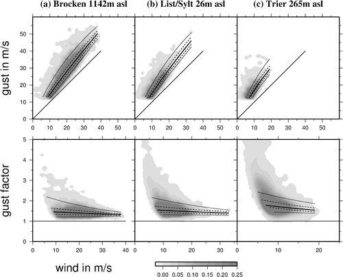
For this purpose, the Gauss-filtered density of observations in the (v _10m – v _max)-space using 1/e-filter-widths of 2 m s⁻¹ in each direction was calculated. Fig. 2 shows density plots of wind gusts against mean wind speeds and gust factors for three exemplary sites: one representative of an exposed mountain region, one for a coastal area and one for a low-range hilly region far from the coast. In addition, quantile regression lines based on a Weibull-like behaviour of the distribution of gust factors, dependent on wind speed above a certain level and assuming an exponential power-law relation between average wind speed and gusts (see Appendix A.2), have been added to the diagrams. The medians of the gust factors vary only little as a function of wind speed, showing very weak negative slopes in all cases. This behaviour may be attributed to the fact that strong wind conditions lead to near-neutral stratification with less variable TKE/wind speed relations. While the median of the gust factors is relatively similar for different locations, the spread of the gust factors’ distribution at constant wind speed is obviously very variable: The width of the distributions of gust factors depends strongly on wind speed, and it increases with decreasing mean wind speed (see Fig. 2).

Fig. 2.  Density plots of gust versus 10 m wind speed (upper row) and gust factors versus 10 m wind speed (lower row) for three exemplary climate observation sites, representative for an exposed mid-range mountain (Brocken, 10453), a maritime/coastal region (List/Sylt, 10020) and a low-range hilly region far from the coast (Trier, 10609). Colour shades represent normalised density of observations, lines represent a quantile regression of the gust factors for the 5, 25, 50, 75 and 95% quantiles. For more details on each station, see Table 1.

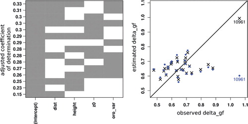
In Fig. 3, the spatial variation of the estimated mean gust factors is depicted for the observational sites. For this graphic, 10 sites with low counts of gust observations were excluded. The dependence of mean gust factors − given as quantiles – from latitude and height are shown as graphs, a map of Central Europe shows the location of the sites and corresponding average median values. The box and whiskers, showing 5, 25, 50, 75 and 95% quantiles (q05, q25, q50, q75 and q95), give an idea of the width of the gust factors distribution. The first conclusion apparent from the data is that there is no clear relation of the gust factor or its spread with latitude or elevation of observational sites. Extremely exposed mountain observations (10453 and 10908) are connected with rather small gust factors. This may be primarily attributed to the fact that in the free atmosphere, weaker turbulence is connected with higher average wind speeds. As it would be useful to relate the gust factors with external parameters of the land cover, linear models between the median gust factor and potential predictors were tested. Only those parameters that reveal at least a weak relationship are depicted in Fig. 3, namely, the location and the height of observational sites. A slight increase of gust factors with increasing distance to the coast from 1.45 to 1.65 may be observed in Fig. 3a. This increase is statistically significant at the 95% level (after student's t-test), but the explained variance is only 11%. A multilinear model using height of observational sites and their location as predictors gains with a coefficient of determination of 13%, again not a promising result for a potential predictive skill of a statistical spatial interpolation. More interesting than a gust factor itself may be the spread, which is formed by the difference between q95 and q05. This is a direct measure for the width of the gust factors distribution and for the uncertainty at which a gust factor can be estimated, which may be associated with local topographic characteristics. In order to test for the predictability of the (q95–q05)-spread, a second multilinear model has been tested. It uses the difference of quantiles (q95–q05) as predictand and distance from the German Bight, height, roughness length (z0) and orographic variance within a circle of 10 km diameter as predictors (Fig. 4). The topographic characteristics were derived from USGS GTOPO30 and USGS Global Land Cover Characterisation 1 km land cover database. For this purely statistical model, a coefficient of determination (COFD, comparable to explained variance) of roughly 33% could be reached (Fig. 4a, topmost row). The predictability is higher than for the gust factor itself, but for a possible spatial interpolation the results are not convincing, indicating that such a statistical method needs improvement. Interestingly, roughness plays only a minor role for the predictive skill.

Fig. 3.  (a) Mean gust factors at observational sites (x-axis) against latitude. (b) Mean gust factors against heights of observational sites. The box and whiskers show mean values for the 5, 25, 50, 75 and 95% quantile, respectively. (c) Mean 50% quantiles of the gust factors are depicted as colour dots on their geographical location. Ten stations with very low numbers of observations have been excluded from this plot. For more details on each station, see Table 1.

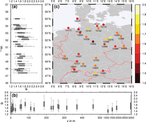
Fig. 4.  Evaluation of the MLR model for the width of local gust factor distributions. Predictors are distance from the German Bight (dist), height of the site (height), roughness length at the site (z0) and orographic variance within a circle of 10 km diameter (oro_var). (a) Adjusted coefficient of determination (COFD, left axis) for different combinations of predictors, ranked by their performance in terms of the COFD: the predictors used for each one model (rows) are marked with grey boxes. The best model with the highest COFD uses all predictors except roughness length (topmost row). (b) Scatter plot of the estimated and observed values by the optimum model. Crosses mark estimates of the full calibration; blue dots mark a cross-validation by leaving out data of the site. The station ‘Zugspitze’ is marked with the station number 10961.

It has to be concluded that the gust factor seems to be strongly connected with dynamical features like wind speed or TKE, which have to be taken from model simulations. Still, an important result from Figs. 2 and 3 is that, in a first order approximation, the consideration of probabilities by using quantile regression parameters of the gust factors with wind speed obtained for the specific sites, where a comparison of gusts is intended, provides more appropriate information than classical empirical gust estimation. This is further discussed in Section 4.4, Fig. 8.

4.2. Overall evaluation of COSMO-CLM storm simulations

First, the performance of the COSMO-CLM storm simulations is discussed by comparing the paths of the storms in the RCM simulations with tracks derived directly from ERA-Interim data (see Section 2). Although ERA-Interim has a lower resolution, tracks of the storms obtained from these data are the best available estimate of storm positions and intensities. For the comparison with the COSMO-CLM results, core pressure is considered as a measure of intensity. The COSMO-CLM cyclone tracks are simply constructed from minimum pressure near the ERA-Interim cyclone track, which is sufficient, as the number of tracked cyclones within the RCM domain is limited, and the track can thus be identified unequivocally. Comparison is done only for the segment of the cyclone track within the COSMO-CLM domain.

The comparison of the tracks is shown in Table 2 and Fig. 5. In Table 2, characteristics of the 10 strongest cyclones for the ERA-Interim period from 1989 to 2007 – in terms of potential damage over Germany (cf. Pinto et al., 2007a; Fink et al., 2009) calculated from reanalysis data – are compared for reanalysis and COSMO-CLM simulations. Except for Daria (24 January 1990), the core pressure values are in good agreement. Fig. 5 exemplarily shows four cyclone tracks following very different paths with different intensities and characteristics (Daria, Barbara, Lothar, Kyrill). Results document that the tracks are generally in very good agreement. However, and particularly for cases when the track includes open systems during life-time, that means a vorticity minimum without closed isobars (like, for example, Lothar) on the reanalysis grid, the tracks may differ considerably, which does not come unexpectedly.

Fig. 5.  Storm tracks, storm footprints (maximum wind gust speed during the event) and series of minimum pressure for four of the strongest storm events simulated with the COSMO-CLM (green tracks, colour-shaded gust speed in m s⁻¹), in comparison to ERA-Interim Reanalysis (black tracks). The lower panels show time series of sea level pressure in hPa, x-axis is longitude. The dots mark six-hourly steps, which is the resolution of ERA-Interim, but COSMO-CLM tracks have been drawn hourly. All tracks were limited to the parts that lie entirely inside the COSMO-CLM domain. (a) Daria, 25 January 1990, (b) Verena, 14 January 1993, (c) Lothar, 26 December 1999 and (d) Kyrill, 18 January 2007.

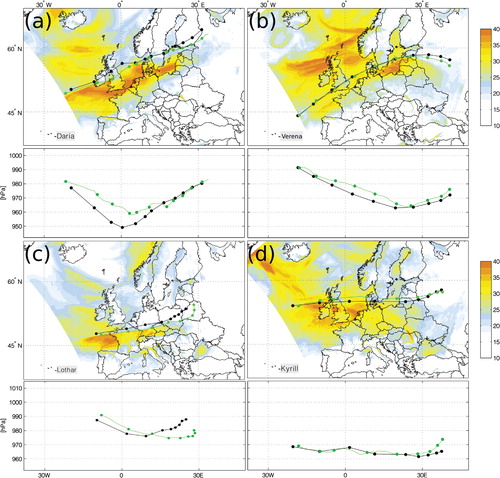
Table 2. Key features of the tracks of the strongest 10 storms (see text) simulated with CCLM

Storm	CCLM			ERA-Interim
	Date	Lat (°N) Lon (°E)	P min (hPa)	Date	Lat (°N) Lon (°E)	P min (hPa)
Daria	25 January 1990 21UTC	56.43°N 4.63°E	958.02	25 January 1990 18UTC	56.82°N 0.42°E	949.13
Vivian	27 February 1990 12UTC	61.72°N 19.09°E	938.86	27 February 1990 12UTC	60.67°N 21.14°E	941.04
Wiebke	1 March 1990 03UTC	52.46°N 11.28°E	976.01	1 March 1990 06UTC	52.26°N 18.95°E	971.8
Verena	14 January 1993 10UTC	58.31°N 23.67°E	973.68	14 January 1993 06UTC	57.76°N 19.53°E	973.07
Barbara	24 January 1993 05UTC	59.97°N 3.00°E	965.43	24 January 1993 00UTC	59.17°N 3.74°W	966.8
Anatol	4 December 1999 00UTC	57.43°N 18.06°E	958.15	3 December 1999 18UTC	56.96°N 9.67°E	956.42
Lothar	27 December 1999 00UTC	51.39°N 22.82°E	974.75	26 December 1999 12UTC	50.46°N 9.37°E	976.09
Jeanett	27 October 2002 14UTC	56.32°N 7.06°E	977.86	27 October 2002 12UTC	56.44°N 4.05°E	975.32
Kyrill	19 January 2007 02UTC	56.47°N 24.01°E	962.97	19 January 2007 06UTC	56.00°N 28.54°E	961.51
Emma	29 February 2008 21UTC	62.72°N 1.14°W	956.45	29 February 2008 18UTC	62.34°N 4.66°W	959.97

Shown is the date and time, at which the minimum sea level pressure P _min occurred, the geographical position and the minimum pressure value. The storms are in chronological order.

4.3. Comparison of various WGE formulations for single storms

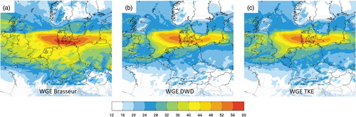
In this paragraph, results of WGE methods are compared. Fig. 6 shows footprints of storm ‘Anatol’ (3 December 1999; cf. Ulbrich et al., 2001). These footprints depict the maximum wind gust for each model grid point during the whole storm episode, thereby providing a wind gust ‘signature’ of the storm. Comparing the panels Fig. 6a–c, the WGE Brasseur (Fig. 6a) estimates highest wind speeds with little land–sea differences, while the two other methods provide very similar patterns (Fig. 6b, c). This is the case for the area primarily affected by the cyclone (North Sea, Denmark and Baltic Sea) and nearby areas (e.g. Germany). Over water, differences between WGE methods are smaller. Over land, WGE Brasseur shows less reduction in gust speed and, thus, estimates higher gusts compared with WGE DWD and WGE TKE. An overestimation of gusts is also apparent in Brasseur (2001) and seems to be confined to storms, whereas less extreme situations are represented well.

Fig. 6.  Patterns of WGE for storm Anatol (a) WGE Brasseur, (b) WGE DWD and (c) WGE TKE. For further details, see text.

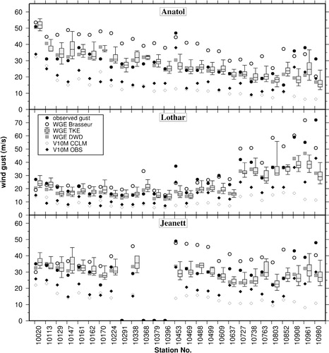
In Fig. 7, WGE for three exemplary storms and all available gust observations are shown. Also, mean 10 m wind speeds simulated and from observations are depicted, in order to see if gust over- or under-estimation corresponds to a similar failure in the average wind speed. As expected from Fig. 6, the WGE Brasseur method overestimates gusts in high wind speed situations with gusts larger than 30 m s⁻¹, except at mountain sites, where it fits better to the observations. For gust speeds below 30 m s⁻¹, this systematic overestimation cannot be seen. On the other hand, for storm Lothar (26 December 1999), which had an impact far away from coastal regions in Germany (e.g. Ulbrich et al., 2001), results of WGE Brasseur were in better agreement with the other WGE methods than for storms moving over the North/Baltic Seas (e.g. Kyrill or Anatol). WGE DWD and the probabilistic estimate with the WGE TKE are relatively similar and generally, but not always, in better concordance with observations. Deficiencies are mostly related to failures in model prediction, as the comparison with mean 10 m wind speeds shows: Both WGE DWD and the probabilistic WGE TKE approach fail if the mean 10 m wind is not predicted correctly (e.g. station 10980 for storm Lothar). The width of the 90% interval of the WGE, marked by the difference of the quantiles q05 and q95, is typically 10 m s⁻¹, reaching also values of 20 m s⁻¹ at mountain sites (10961 Zugspitze, 10980 Wendelstein), and sometimes at coastal stations (10129 Bremerhaven, 10147 Hamburg). The spread of the gusts uncertainty range depends on the average turbulent wind speed , therefore, it is varying in both time and space. With respect to possible damage estimation from WGE, the large uncertainty indicates that the consideration of probabilistic aspects might be useful.

Fig. 7.  Wind speed of gusts and 10 m winds at all available observational sites for three exemplary storms, Anatol (3 December 1999), Lothar (26 December 1999) and Jeanett (27 October 2002). The standard WGE methods after Brasseur (2001) (WGE Brasseur) and Schulz and Heise (2003) (WGE DWD) are compared with the TKE-based probabilistic estimation (box and whiskers for 5, 25, 50, 75 and 95% quantiles, respectively). The difference between 5 and 95% quantiles mark the range in which 90% of gusts are expected to occur. The latter are slightly shifted for easier comparison. For more details on each station, see Table 1.

4.4. Computation of skill scores for the whole storm sample

Next, an overall evaluation of WGE methods is performed taking as many historical storms into account as the observations allow (up to the end of 2005). For the calculation of the scores, only maximum wind gusts per event were considered, which reduces the effects of temporal phase shifts of a storm event. The three scores aim at three different aspects of quality: The QSS evaluates the form of the gust distribution without any emphasis on the temporal correlation of model data with observations; the RSS quantifies the effect of deviation between model and observations, the correlation CORR only evaluates temporal coincidence. Because QSS and RSS require a reference method for comparison, a WGE using a spatially varying, but temporary constant gust factor from Fig. 3 is defined as reference method. As Fig. 8 shows, the Brasseur-type WGE has a less good performance than the TKE-based WGEs, except at mountain sites. At some locations, WGE Brasseur is even worse than the constant gust factor. WGE DWD and the probabilistic TKE approach, where only the median value has been considered for scores, behave in a very similar way. Overall, the WGE DWD shows in this study slightly better skill scores than the other approaches (Table 3), although the difference to the probabilistic WGE TKE is – due to the same physical base of both approaches – very small. The good performance of the WGE DWD could be expected, as this method was developed for Germany by the DWD. It has been slightly tuned by choosing 30 m instead of 10 m in the original formulation as reference height for available momentum and TKE in the Prandtl-layer of the model. Even though the WGE Brasseur method performs, in general, less well in this comparison, it has to be stated that the potential of fine-tuning has not been performed for this study. The consideration of a changed numerical implementation may counteract the overestimation of this WGE (not shown) and provides more comparable results to the other methods.

Fig. 8.  Skill scores for the quality of the statistical distributions of gusts (QSS), the deviation of gust estimates from observations (RSS) and for temporal coincidence (CORR) at climate observation sites in Germany for WGE Brasseur (light grey), WGE TKE (dark grey) and WGE DWD (black). On the last row, an average over all stations per approach is given. For each station, the maximum number of considered storms is limited by availability of observations. M indicates a mountain station (height above 800 m a.s.l.). For more details on each station, see Table 1.

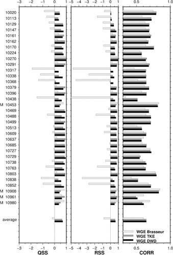
Table 3. Averaged skill scores for all stations and all events using investigated WGE methods

	DWD	TKE	Brasseur
QSS	0.69	0.63	−0.24
RSS	0.63	0.57	−0.96
CORR	0.65	0.65	0.60

See text for details on skill scores and different WGE formulations.

5. Discussion

Our results indicate that the three different WGE approaches may provide quite diverse results. However, a main finding is that the WGE Brasseur approach produces results, which differ from the other two methods. Further, WGE DWD and WGE TKE deliver very similar gust patterns and time series. Such behaviour could be expected, as the WGE Brasseur is in general methodically different from the others. WGE Brasseur overestimates wind gusts in flat terrain, whereas skill scores even suggest a better performance at mountain sites (cf. also Pinto et al., 2009). However, although fine-tuning for WGE parameters and formulation of the discretisation has not been performed extensively in this study, results indicate that the quality of WGE may be improved by further calibration. From this point of view, a general quality statement on the methods may be debatable; only the actual realisation (in our case an implementation in the COSMO-CLM model) can be rated.

Due to their intrinsic characteristics, WGE Brasseur and WGE DWD can be applied in every grid cell of an NWP model and are able to deliver high-resolution estimates of gust patterns. Nevertheless, the calibration evaluation is confined to observational sites; also for the WGE TKE, the probabilistic assessment of uncertainty ranges is based on local observations. The spatial interpolation of WGE TKE is in principle possible, but using less sophisticated approaches – simple MLRs using fixed topographic characters as predictors – it provides not satisfying results. Although statistical characteristics of the distribution are expected to depend very much on local topographic effects related to land cover (in terms of roughness length) or exposition, height and land-use in the nearest region of the observation sites (among other factors), dynamic factors like prevailing wind direction leading to advection of TKE and, of course, TKE itself seem to be more important for a predictive skill of a spatial interpolation model. All these factors are potential predictors in a multiple, not necessarily linear, regression model, which would have to be applied within the atmospheric model. An ‘offline’ version of a MLR model, which takes four topographic characteristics into account but which neglects dynamic forcing, is not a satisfying option to spatially interpolate uncertainties in terms of the width of local gust factor distributions (see Section 4.1). A satisfying interpolation technique (similar to Haas and Born, 2011), considering further dynamical parameters, requires far more attention than the present article can provide. Therefore, an interpolation of the statistical characteristics of gustiness between observational sites is not provided here and is left for future work.

As already stated, the WGE TKE method and the WGE DWD implementation behave very similar in terms of the skill scores. The time series of observed and simulated wind speeds indicate that gusts cannot be predicted correctly if the NWP model already underestimates mean wind speeds. Relatively small displacements of wind patterns, for example, connected with the cold front passage, result in large discrepancies between observations and simulated gusts. Differences in temporal behaviour are reduced by considering footprints of storms, that is, the maximum gusts during the storm period, instead of hourly values for calculation of skill scores.

One of the main advantages of the WGE TKE is the consideration of a probabilistic formulation and, thus, of a measure of uncertainty for each value. For example, the 90% uncertainty intervals range from around 10 m s⁻¹ in average to 25 m s⁻¹ at mountain and some coastal stations, making clear that probabilistic interpretation of possible wind-related damages can be important. Thus, such an approach, including a probabilistic assessment of uncertainty ranges, may be of added value not only for issuing appropriate severe weather warnings, but also for application for wind-related damage estimation (e.g. Pinto et al., 2007a, 2010; Della-Marta et al., 2010; Schwierz et al., 2010) and wind energy estimates (e.g. Barthelmie et al., 2008; Pryor and Barthelmie, 2010).

6. Summary and conclusions

The present study compares three WGE methods with respect to their forecast quality using different skill scores representing the similarity of probability distributions, the standard error and the temporal correlation. Two of the WGE methods estimate gusts locally from mean wind speed and the turbulence state of the atmosphere (WGE DWD and WGE TKE), the third one named after Brasseur (2001) represents a mixing-down of high momentum within the PBL. The proposed WGE TKE permits a probabilistic interpretation using statistical characteristics of gusts at observational sites for an assessment of uncertainty. The WGE methods are implemented in the regional climate model, COSMO-CLM, which has been applied to 158 windstorms of the last four decades. The WGE methods are applied for each time step, calculating the maximum gust during every output interval. WGEs are compared with gust observations at 37 observational sites in Germany.

In terms of all skill scores, the two local WGE methods show an overall better behaviour. WGE Brasseur shows hardly a reduction of gust wind speeds over land compared with sea, leading to an overestimation between gusts over flatland and moderately hilly regions. The Brasseur method has only better skill scores for mountain stations and in situations with weaker winds. The potential of fine-tuning has not been applied in this study. In fact, extensive calibration and theoretical superiority may be competing effects: a theoretically more appropriate method may be worse in practice than any well fitted approach.

For historical reasons, a lot of WGE methods do not take TKE into account directly. The results of the present study document that using TKE as parameter for gust estimation is especially valuable for NWP models, which supply TKE as prognostic or diagnostic variable. Without extensive tuning, WGE TKE is able to predict gusts at a comparable quality as the WGE DWD method. For cases when no TKE can be used directly or in a diagnostic way, estimates of atmospheric static stability may provide better results than constant gust factors. However, physically based methods should be preferred. The TKE formulation has the advantage that it allows for a ‘native’ interpretation of wind gusts as a result of local TKE. Thus, we propose that the consideration of a probabilistic WGE TKE approach in NWP models may have several advantages towards other methods, particularly as it allows for an estimation of uncertainties.

The WGE TKE method introduced in this work does not consider either fine-tuning or spatial interpolation. While the fine-tuning may not be of general interest, as its usefulness may be restricted to the fitted region and the particular NWP model characteristics, the spatial interpolation may be valuable for an improvement of gust estimations in regions with insufficient observations. Because of the unknown portion of the impact of local topographic characteristics, this interpolation has to be carried out very carefully and will be the objective of future work.

7. Acknowledgements

This research has been funded by the German Association of Insurers (‘Gesamtverband der Deutschen Versicherungswirtschaft’, GDV) in a project dealing with the impacts of climate change for the insurance industry for Germany (‘Auswirkungen des Klimawandels auf die Schadensituation in der deutschen Versicherungswirtschaft’). Model simulations have been performed at the Computing Centre of the Cologne University (RRZK) and the German Climate Computing Centre (DKRZ). We thank the European Centre for Medium Range Weather Forecast (ECMWF, UK) for reanalysis data and the German Weather Service (DWD) for providing synoptic station data. We thank Rabea Haas for helping to prepare Fig. 4 and Sven Ulbrich (both Univ. Cologne) for Fig. 5 and Table 2.

8. Appendix A:

A.1. Basic derivation of turbulence-driven wind gust estimation methods

We propose the use of the near-surface TKE for analysing the relation between average wind speed and wind maxima. This approach is similar to the theory proposed by Wichers Schreur and Geertsema (2008), but it handles the TKE in a different way. Following Reynolds’ concept of separation in average and subscale portions of a variable, e. g. _, the mean kinetic energy consists of one term caused by average winds and another term caused by wind deviations. Using Einstein's summation convention and the definition of average TKE:A.1

can be expressed in terms of the kinetic energy of the mean wind speed ^, and :A.2

Let be the components of the wind gust vector and the wind gust speed, then the definitions and lead to the following decomposition of the maximum kinetic energy available for gusts:A.3

The maximum gust speeds are expected to occur when mean wind and gust vectors have the same direction. Expressing v _max in terms of E _max yields:A.4

In eq. (A.4), q _max may be expressed in terms of the known grid-scale TKE and an unknown, subscale stochastic part. Thus, using as average wind speed, eq. (A.4) may be rewritten as:A.5

with ɛ _v being the square root of the difference between the energy of the wind speed deviation v′ and the TKE:A.6

Equation (A.5) is a key equation for turbulence-driven gust parameterisations, as they all can be expressed using this formula. It is an advantageous formulation for most state-of-the art mesoscale models, as TKE is usually a prognostic variable of the turbulence parameterisation. Equation (A.4) is exact, if ɛ _v is known, which is variable in time and space. The gust factor (g _v ) can then be written as:A.7

The random parts ɛ _v and are also variable both in space and time. In the WGE DWD, eq. (A.5) is approximated using:

with a semi-empirical factor α, based partly on PBL theory considerations (Panofsky and Dutton, 1984) and partly being empirical (see Schulz, 2008; Schulz and Heise, 2003). In WGE TKE, the random part is estimated using the gust observations. Both WGE DWD and WGE TKE interpolate , u* and to a level of 30 m above surface.

A.2. Probabilistic approach of WGE

The simplest way to achieve information about wind gust distributions is to estimate the width of the WGE distribution using mean wind speed dependent quantile functions, which may be assessed by quantile regression. For that purpose, we assume the gust distribution and, thus, the relation between gust factors and mean wind speed to be of exponential power-law type:A.8

The assumed type of the fit function does not affect the results considerably, as long as curvature, slope and intercept are used in the fit. Here, very small or large values are discarded due to data availability, as (1) wind gusts are only reported above 12 m s⁻¹; and (2) for some stations, the largest values are limited to 50 m s⁻¹. The fit of eq. (A.8) can be undertaken via linear regression using:A.9

Equation (A.9) allows for an estimation of parameters b and a by linear quantile regression, which gives an assessment of the form of gust distributions at constant mean wind speed by showing 5, 25, 50, 75 and 95% quantiles (q05, q25, q50, q75 and q95).

A.3. Skill scores

The evaluation of the WGE is undertaken using skill scores. The first and most simple score is the temporal correlation CORR of WGE and observations at weather stations for storm episodes. It reflects the temporal accordance of the two time series without regard to the absolute values. The other two scores are formulated in analogue to the Brier skill score and are designed to compare a method in focus with a reference method. The reference method is the WGE with a spatially varying but temporarily constant gust factor obtained from observations (see Fig. 3); the compared methods are either WGE Brasseur, the WGE DWD or WGE TKE. The basic form of all Brier-type skill scores is:A.10

with different types of error estimates (ɛ, ɛ _ref) for WGE methods and the reference method, respectively. A Brier-type SS is zero for equal quality of both methods; for values below 0, the evaluated method is worse than the reference, and for values larger than 0, the tested method is better than reference with optimum performance at 1. For the RMSE skill score RSS, (ɛ, ɛ _ref) are root mean squared deviations of WGE and gust observations:A.11

WGE is the wind gust estimation after one of the three methods and v _max represents gust observations. The idea is simply that a better WGE should produce less deviation between observed and predicted wind gusts. For the quantile skill score (QSS), (ɛ, ɛ _ref) is the sum of distances of points of ranked time series (WGE_rank, v _max,rank) from the line of identity in a scatter plot:A.12

The scaling factor just indicates that in a scatter diagram of ranked values the length of the shortest path from the point (WGE _rank, v _max,rank) to the line of identity is measured. The QSS evaluates the form of distributions: although temporal correlation may be poor, the ranked events can be similar in a scatter plot.

References

- Agustsson H. Olafsson H. Mean gust factors over complex terrain. Meteorol. Z. 2004; 13: 149–155.
- Agustsson H. Olafsson H. Forecasting wind gusts in complex terrain. Meteor. Atmos. Phys. 2009; 103: 173–185.
- Barthelmie R. J. Murray F. Pryor S. C. The economic benefit of short-term forecasting for wind energy in the UK electricity market. Energy Policy. 2008; 36: 1687–1696.
- Böhm U. Keuler K. Österle H. Kücken M. Hauffe D. Quality of a climate reconstruction for the CADSES region. MetZ. Spec. Iss. Regional Clim. Model. COSMO-CLM (CCLM). 2008; 17(8): 477–485.
- Brasseur O. Development and application of a physical approach to estimating wind gusts. Mon. Wea. Rev. 2001; 129: 5–25.
- Brasseur O. Gallee H. Boyen H. Tricot C. Reply. Mon. Wea. Rev. 2002; 130: 1936–1943.
- Dee, D. P, Uppala, S. M, Simmons, A. J, Berrisford, P, Poli, P and co-authors. 2011. The ERA-Interim reanalysis: configuration and performance of the data assimilation system. Quart. J. R. Meteor. Soc. 137, 553–597. 10.3402/tellusa.v64i0.17471.
- Della-Marta, P. M, Liniger, M. A, Appenzeller C, Bresch D. N, Köllner-Heck P and Muccione V. 2010. Improved estimates of the European winter wind storm climate and the risk of reinsurance loss using climate model data. J. Appl. Meteor. Clim. 49, 2092–2120.
- Della-Marta, P. M, Mathis, H, Frei, C, Liniger, M. A, Kleinn, J and Appenzeller, C. 2009. The return period of windstorms over Europe. Int. J. Climatol. 29, 437–459.
- De Rooy W. C. Kok K. A combined physical statistical approach for the downscaling of model wind speed. Wea. Forec. 2004; 19: 485–495.
- Durst C. D. Wind speeds over short periods of time. Meteorol. Mag. 1960; 89: 181–186.
- Fink A. H. Brücher T. Ermert E. Krüger A. Pinto J. G. The European Storm Kyrill in January 2007: synoptic evolution and considerations with respect to climate change. Nat. Hazards Earth Syst. Sci. 2009; 9: 405–423.
- Friederichs P. Goeber M. Bentzien S. Lenz A. Krampitz R. A probabilistic analysis of wind gusts using extreme value statistics. Meteorol. Z. 2009; 18: 615–629.
- Goyette, S, Brasseur, O and Beniston, M. 2003. Application of a new wind gust parameterisation: multiple scale studies performed with the Canadian regional climate model. J. Geophys. Res. 108(D13), 4374. 10.3402/tellusa.v64i0.17471.
- Haas R. Born K. Probabilistic downscaling of precipitation data in a subtropical mountain area: a two-step approach. Nonlin. Process. Geophys. 2011; 18: 223–234.
- Jaeger, E. B, Anders, I, Lüthi, D, Rockel, B, Schär, C and co-authors. 2008. Analysis of ERA40-driven CLM simulations for Europe. Meteorol. Z. 17, 349–367.
- Klawa M. Ulbrich U. A model for the estimation of storm losses and the identification of severe winter storms in Germany. Nat. Hazards Earth Syst. Sci. 2003; 3: 725–732.
- Lautenschlager, M, Keuler, K, Wunram, C, Keup-Thiel, E, Schubert, M, Will, A, Rockel, B and Boehm, U. 2009. Climate simulation with CLM, scenario A1B run no.1, data stream 3: European region MPI-M/MaD. World Data Center Clim. 10.3402/tellusa.v64i0.17471.
- Mellor G. Yamada T. Development of a turbulence closure model for geophysical fluid problems. Rev. Geophys. Space Phys. 1982; 20: 851–875.
- Murray R. J. Simmonds I. A numerical scheme for tracking cyclone centres from digital data. Part I: development and operation of the scheme. Aust. Meteorol. Mag. 1991; 39: 155–166.
- Nissen, K. M, Leckebusch, G. C, Pinto, J. G, Renggli, D, Ulbrich, S and Ulbrich, U. 2010. Cyclones causing wind storms in the Mediterranean: characteristics, trends and links to large-scale patterns. Nat. Hazards Earth Syst. Sci. 10, 1379–1391.
- Panofsky, H. A and Dutton, J. A. 1984. Atmospheric Turbulence: Models and Methods for Engineering Applications. John Wiley & Sons: New York, 397 pp.
- Pinto J. G. Fröhlich E. L. Leckebusch G. C. Ulbrich U. Changes in storm loss potentials over Europe under modified climate conditions in an ensemble of simulations of ECHAM5/MPI-OM1. Nat. Hazards Earth Syst. Sci. 2007a; 7: 165–175.
- Pinto J. G. Neuhaus C. P. Krüger A. Kerschgens M. Assessment of the wind gust estimates method in mesoscale modelling of storm events over West Germany. Meteorol. Z. 2009; 18: 495–506.
- Pinto J. G. Neuhaus C. P. Leckebusch G. C. Reyers M. Kerschgens M. Estimation of wind storm impacts over West Germany under future climate conditions using a statistical-dynamical downscaling approach. Tellus A. 2010; 62: 188–201.
- Pinto J. G. Spangehl T. Ulbrich U. Speth P. Sensitivities of a cyclone detection and tracking algorithm: individual tracks and climatology. Meteorol. Z. 2005; 14: 823–838.
- Pinto, J. G, Ulbrich, U, Leckebusch, G. C, Spangehl, T, Reyers, M and Zacharias, S. 2007b. Changes in storm track and cyclone activity in three SRES ensemble experiments with the ECHAM5/MPI-OM1 GCM. Clim. Dyn. 29, 195–210.
- Pryor S. C. Barthelmie R. J. Climate change impacts on wind energy: a review. Renewable and Sustainable Energy Reviews. 2010; 14: 430–437.
- Ritter B. Geleyn J.-F. A comprehensive radiation scheme of numerical weather prediction with potential application to climate simulations. Mon. Wea. Rev. 1992; 120: 303–325.
- Rockel, B, Will, A. and Hense, A. 2008. Special issue: regional climate modelling with COSMO-CLM (CCLM). Meteorol. Z. 17, 347–348.
- Schulz, J.-P. 2008. Revision of the turbulent gust diagnostics in the COSMO model. COSMO Newslett. 8, 17–22. Online at: www.cosmo-model.org.
- Schulz, J.-P and Heise, E. 2003. A new scheme for diagnosing near-surface convective gusts. COSMO Newslett. 3, 221–225. Online at: www.cosmo-model.org.
- Schwierz, C, Köllner-Heck, P, Zenklusen Mutter, E, Bresch, D.N, Vidale, P.-L, Wild, M and Schär, C. 2010. Modelling European winter wind storm losses in current and future climate. Clim. Change. 101, 485–514. 10.3402/tellusa.v64i0.17471.
- Simmonds, I, Murray, R. J and Leighton, R. M. 1999. A refinement of cyclone tracking methods with data from FROST. Aust. Met. Mag. Special Edition. 35–49.
- Steppeler, J, Dom, G, Schättler, U, Bitzer, H. W, Gassmann, A and co-authors. 2003. Meso-gamma scale forecasts using the nonhydrostatic model LM. Meteorol. Atmos. Phys. 82, 75–96.
- Ulbrich, U, Fink, A. H, Klawa, M and Pinto, J. G. 2001. Three extreme storms over Europe in December 1999. Weather. 56, 70–80.
- Uppala, S. M, Kallberg, P, Hernandez, A, Saarinen, S, Fiorino, M and co-authors. 2005. The ERA-40 reanalysis. Quart. J. R. Meteor. Soc. 131, 2961–3012.
- Verkaik, J. W. 2000. Evaluation of two gustiness models for exposure correction values. J. Appl. Meteor. 39, 1613–1626.
- Wichers Schreur, B and Geertsema, G. 2008. Theory for a TKE based parameterization of wind gusts. HIRLAM Newslett. 54, 177–188. Online at: http://hirlam.org/index.php?option=com_docman&Itemid=70.
- Wieringa J. Gust factors over open water and built up country. Bound. Layer Meteor. 1973; 3: 424–441.