A modified atmospheric non-hydrostatic model on low aspect ratio grids

Abstract

It is popular to use a horizontal explicit and a vertical implicit (HE-VI) scheme in the compressible non-hydrostatic (NH) model. However, when the aspect ratio becomes small, a small time-interval is required in HE-VI, because the Courant-Fredrich-Lewy (CFL) criterion is determined by the horizontal grid spacing. Furthermore, simulations from HE-VI can depart from the forward–backward (FB) scheme in NH even when the time interval is less than the CFL criterion allowed. Hence, a modified non-hydrostatic (MNH) model is proposed, in which the left-hand side of the continuity equation is multiplied by a parameter δ (4≤δ≤16, in this study). When the linearized MNH is solved by FB (can be other schemes), the eigenvalue shows that MNH can suppress the frequency of acoustic waves very effectively but does not have a significant impact on the gravity waves. Hence, MNH enables to use a longer time step than that allowed in the original NH. When the aspect ratio is small, MNH solved by FB can be more accurate and efficient than the NH solved by HE-VI. Therefore, MNH can be very useful to study cloud, Large Eddy Simulation (LES), turbulence, flow over complex terrains, etc., which require fine resolution in both horizontal and vertical directions.

• non-hydrostatic model
• forward-backward
• HE-VI
• eigenvalue
• LES
• aspect ratio

1. Introduction

Atmospheric non-hydrostatic (NH) models have been used to study small-scale meteorological phenomena, including convection, turbulence, mountain waves, clouds, hurricane, etc. The fine resolution models also become popular in numerical weather prediction. With the increase of computing resources, the model horizontal resolutions increase drastically, and the aspect ratio approaches unity as in cloud and turbulence models. The numerical schemes applied in various NH models have been discussed by Saito (2007). This study will compare the results of modified non-hydrostatic (MNH) model solved using forward–backward (FB) scheme and results of NH model solved using FB and horizontal explicit and vertical implicit (HE-VI) scheme (Klemp and Wilhemson, 1978). In the shallow water system, FB scheme was obtained by first integrating the gravity wave terms of either the equations of motion or the continuity equation forward, and then those of the other equations backward in time (Mesinger and Arakawa, 1976). The FB scheme was applied to study the motions in the atmosphere as reported by Gadd (1978), Sun (1980, 1984) and others. In both FB and HE-VI schemes, internal gravity waves are solved in a short time step Δts, while the low-frequency modes and physical processes are treated in a longer time step Δtb. When the horizontal grid spacing is twice or larger than the vertical, the results from HE-VI with a larger Δts are almost identical to those from FB with a smaller Δts. On the other hand, if the vertical and horizontal grid spacings are comparable, HE-VI is limited by the CFL criterion of the acoustic waves propagating horizontally. Furthermore, the numerical simulations from HE-VI can be quite different from FB even with the same time interval shorter than the CFL allowed. It may indicate that the popular HE-VI is inappropriate when the aspect ratio is small or the horizontal gradient is comparable with the vertical gradient.

Many approximations of the original Navier–Stokes equations have been introduced, including anelastic approximation, hydrostatic approximation, quasi-geostrophic approximation, etc. MacDonald et al. (2000) developed a quasi-non-hydrostatic model (QNH). It is characterised by a parameter, α (typically the square of the vertical to horizontal aspect ratio), which multiplies the hydrostatic terms in the vertical equation of motion. The important effect of the QNH parameter is to decrease both the frequency and amplitude of gravity waves, which enables to calculate the vertical equations explicitly in a longer time step. A weakness of the approach is that the hydrostatic adjustment process is slowed down. Here, a modified model, MNH, is proposed to suppress the frequency of acoustic waves by multiplying a parameter δ in the continuity equation. The approximation with δ>1, in this study, is also one of the approximations of the Navier–Stokes equations. When δ=1, MNH is identical to NH. Since FB is applied to solve NH and MNH, we will use FB with different values of δ, and also refer FB as MFB if δ>1. The MFB reduces the frequency of acoustic waves significantly, but much less on gravity waves. The accuracy of MFB increases with the decrease of spatial interval for the same δ. The non-linear NH model Cloud Resolving Storm Simulator (CReSS, Tsuboki and Sakakibara, 2002, 2007) shows that the Kelvin–Helmholtz instability, thermal bubble and mountain waves simulated from the conventional FB can be well reproduced by MFB with a much longer Δts. The MFB was also successfully applied to the National Taiwan University (NTU)-Purdue NH model (Hsu and Sun, 2001; Sun and Hsu, 2005; Sun et al. 2009; Hsieh et al. 2010; etc.) to simulate the mountain waves, lee-vortices, thermal convection, land-sea breeze, etc. It is also noted that other numerical schemes, for example: with the same δ, the modified leapfrog scheme (Sun and Sun, 2011) or the new semi-implicit scheme (Sun, 2011), can be applied to the wave-related terms of MNH to achieve the same efficiency as MFB used in this study.

2. Basic and linearized equations

Following MacDonald et al. (2000), the 2-D NH equations can be written as:2.1 2.2 2.3 2.4 2.5 2.6

where u and w are the x and z components of wind, p is pressure, θ is potential temperature, T is temperature, ρ is density, R is gas constant, C _p is specific heat capacity; D _u and D _w are turbulent diffusions along x and z direction and D _θ is the heat diffusion. The linearized equations (with α=1) become:2.7 2.8 2.9 2.10 2.11

where primes are deviations from the basic state variables (with subscript ‘0’), which are a function of height only, and . The basic state wind is assumed to be 0 for simplicity. Following Hsu and Sun (2001), we obtain:2.12 2.13 2.14 2.15

where:

Here, a parameter δ>1 has been introduced in the continuity equation intended to suppress the frequency of acoustic waves. The theoretical and numerical results will demonstrate that a certain range of this parameter allows a larger time step without deteriorating accuracy. The solutions for differential in time and difference in space are assumed:2.16

The dispersive relationship is:2.17

where:

The solution of eq. (2.17) is:2.18

which includes the sound wave and internal gravity wave . Let us define Φ:

If δΦ<1, eq. (2.18) consists of the acoustic wave:2.19a

and the gravity waves:2.19b

Equations (2.19a, b) show that if δ≥2, damping on frequency of acoustic wave is significant, but it is not severe on gravity wave if . The error of the gravity wave seems acceptable with δ≤16 used in this study from both eigenvalue analysis and non-linear model simulations. The accuracy of gravity waves increases when a smaller value of δ and/or finer space intervals are applied in the model according to eq. (2.19b). The value of σ_g  (δ=1) will be used to compare with the frequency obtained from the MFB and HE-VI schemes in Section 3.

3. Eigenvalue of finite difference equations

The solutions of eqs. (2.12)–(2.15) can be assumed in the following form:3.1

3.1. The finite difference form of FB

When the forward in time is applied to the momentum fields and backward to the pressure and temperature, the finite difference equations of eqs. (2.12)–(2.15) become:3.2 3.3 3.4 3.5

The eigenvalue of eqs. (3.2)–(3.5) is:3.6

Equation (3.6) also consists of two acoustic waves and two gravity waves, as discussed in Hsu and Sun (2001). Let us define:3.7

The amplification factor of eq. (3.6), ∣λ∣, is unity if Δt≤Δt _δ . The frequency ω can be defined by:3.8a

and:3.8b

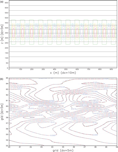
With g=10 m s⁻², C=300 m s⁻¹, Δx=1000 m, Δz=500 m, S ₀=1.0×1.0⁻⁵ m⁻¹ and δ=1, we obtain Δt _δ=1=1.49 s according to eq. (3.7). We also find that when Δt≤Δt _δ=1=1.49 s, the amplification factor is 1. The frequency ω _δ=1 obtained from eq. (3.8) at δ=1 and Δt=1.49 s and the difference from the differential-difference equations, ω _δ=1−σ _g , [σ _g =σ _g  (δ=1) ] are shown in Fig. 1a, in which ω _δ=1≈σ _g and the error is less than 7×10⁻⁸ s⁻¹. The frequency of MFB with δ=4 and Δt=2.98 s (ω _δ=4) and (ω _δ=4−σ _g )≤1.1×10⁻⁵ s⁻¹ are shown in Fig. 1b; frequency of MFB with δ=16 and Δt=5.96 s, (ω _δ=16), and (ω _δ=16−σ _g )≤5.5×10⁻⁵ s⁻¹ are shown in Fig. 1c.

Fig. 1.  Frequency of gravity wave with g=10 m s⁻², C=300 m s⁻¹, Δx=1000 m, Δz=500 m and S ₀=1.0⁻⁵ m⁻¹: (a) ω _δ=1 (with Δt=1.49 s, solid line) and ω _δ=1−σ _g (dash line); (b) ω _δ=4 (with Δt=2.98 s) and ω _δ=4−σ _g and (c) ω _δ=16 (with Δt=5.96 s) and ω _δ=16−σ _g .

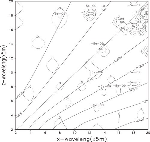
When g=10 m s⁻², C=300 m s⁻¹, Δx=5 m, Δz=5 m and S ₀=1.0×1.0⁻⁵ m⁻¹, the frequency of MFB, ω _δ=16, with δ=16 and Δt=4.71×10⁻² s; and ω _δ=16−σ _g are shown in Fig. 2. The value of ω _δ=16−σ _g is between −2.5×10⁻⁸ and 2×10⁻⁸ s⁻¹, which is much smaller than those in Fig. 1b–c, because of a small spatial interval, as discussed previously.

Fig. 2.  ω _δ=16 (solid line) with Δt=1.179×10⁻² s, Δx=Δz=5 m; and ω _δ=16−σ _g (dotted line) is from −2.5×10⁻⁸ to 2×10⁻⁸ s⁻¹ with contour interval of 5×10⁻⁹ s⁻¹.

3.2. The finite difference form of the HE-VI

The finite difference equations of the explicit scheme for temperature and the horizontal velocity, but implicit in the vertical for w and p can be written as:3.9 3.10 3.11 3.12

The eigenvalue is given by the following equation:3.13

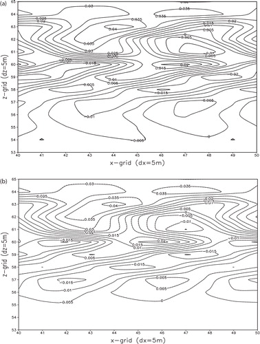
With g=10 m s⁻², C=300 m s⁻¹, S ₀=1.0×1.0⁻⁵ m⁻¹ and δ=1, the frequency ω _H of the gravity waves derived from eq. (3.13) and ω _H −σ _g are shown in Fig. 3a, with Δx=1000 m, Δz=500 m and Δt=2.98 s. The amplification factor is unity. The error of frequency departing from σ _g is from 5×10⁻⁸ to 4×10⁻⁷ s⁻¹. The accuracy is between FB shown in Fig. 1a (δ=1 and Δt=1.49 s) and Fig. 1b (δ=4 and Δt=2.98 s). It is also noted that the conventional FB (δ=1) becomes unstable when Δt=2.98 s. HE-VI also becomes unstable when Δt=5.96 s.

Fig. 3.  (a) ω _HE-VI with Δx=1000 m, Δz=500 m, Δt=2.98 s and ω _HE-VI−σ _g (dash line), contour interval is 5×10⁻⁸ s⁻¹; (b) same as (a) except Δx=Δz=5 m, Δt=1.179×10⁻² s, contour interval of dotted lines is 1×10⁻⁷ s⁻¹.

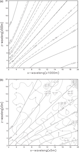
Figure 3b shows the frequency ω _H and ω _H −σ _g , with Δx=Δz=5 m and Δt=1.179×10⁻² s. The difference is between −3×10⁻⁷ and 4×10⁻⁷ s⁻¹, which is much larger than ω _δ=16−σ _g , the MFB with δ=16 and Δt=4.71×10⁻² s as shown in Fig. 2. With Δt=2.357×10⁻² s and Δx=Δz=5 m, HE-VI becomes unstable and the amplitude reaches 5.5 (not shown), because it does not satisfy the CFL criterion for the acoustic waves propagating horizontally.

It is noted that the MFB does not guarantee mass conservation. The HE-VI does not conserve the mass either, because calculation of u ⁿ⁺¹ is based on p ⁿ , but w ⁿ⁺¹ based on p ⁿ and p ⁿ⁺¹. Furthermore, Newtonian damping is often applied to the top and lateral boundaries in NH models, which also destroys the conservations of mass inside the domain. If conservation of mass is required, a variation method proposed by Sun and Sun (2004), and Sun (2007) can be applied.

4. Numerical simulations

The FB with δ=1, 4 and 16, and HE-VI have been incorporated in the CReSS (Tsuboki and Sakakibara, 2007) to simulate the 2-D Kelvin–Helmholtz instability, mountain waves and thermal convection of a warm bubble. The CReSS uses Arakawa-C and Lorenz staggered grids for horizontal and vertical grids, respectively. Prognostic variables are 3-D velocity components, perturbations of pressure and potential temperature, water vapour mixing ratio, subgrid scale turbulent kinetic energy (TKE) and cloud physical variables. In the FB version of CReSS, u, v and w are calculated using the forward in time difference, pressure perturbation p′ is calculated using the backward difference with a small time interval (Δts). The non-linear and other forcing terms are calculated at a larger time interval (Δtb=nΔts), and they remain constant during the integration of sound waves. The leapfrog scheme is applied to the advection terms. The model also includes viscosity and divergence damping of the pressure gradient force in the momentum equations. In HE-VI, the forward difference is applied to calculate u and v; then, the implicit scheme is applied to solve w and p′ using the tri-diagonal matrix solver, as discussed in Saito (2007). The detailed equations and numerical schemes are referred to Tsuboki and Sakakibara (2007). There is no analytical solution in the non-linear eqs. (2.1)–(2.6). Since FB with δ=1 (i.e. smallest Δts) is most comparable with the differential equations, the numerical scheme is also consistent with the original equations with least assumptions. Hence, the results of conventional FB will be used as the references to compare with the simulations from HE-VI and MFB.

4.1. Large Kelvin–Helmholtz wave with Δx=10 m and Δz=5 m

The initial x-component wind u is shown in Fig. 4a. The initial background potential temperature and elliptic-type perturbation with the amplitude of −0.4 K, the horizontal and vertical radii of 180 and 60 m are shown in Fig. 4b. Fig. 5a shows the simulated potential temperatures at t=320 s with Δtb=0.4 s, from FB with δ=1, Δts=0.01 s; δ=4, Δts=0.02 s and δ=16, Δts=0.04 s, as well as HE-VI with Δts=0.02 s. The simulations almost coincide among those four simulations. The differences from the reference (i.e. FB with δ=1, Δts=0.01 s) are shown in Fig. 5b–d. The difference is between −0.03 and 0.02 K for MFB with δ=4, Δts=0.02 s; −0.12 and 0.1 K for MFB with δ=16, Δts=0.04 s; and −0.02 and 0.03 K for HE-VI with Δts=0.02 s. The accuracy is comparable between MFB with δ=4, Δts=0.02 s and HE-VI with Δts=0.02 s. They are more accurate than MFB with δ=16, Δts=0.04 s, but both become unstable with Δts=0.04 s. The FB with δ=1 is also unstable when Δts≥0.02 s. Table 1 shows the time variation of the change of total mass from the initial value, i.e. ɛ=[Mass(t)−Mass(t=0)]/Mass(t=0), for HE-VI (with Δts=0.02 s) and MFB (with δ=16, Δts=0.04 s). The variations are quite small and comparable (−7.10142×10⁻⁷≤ɛ≤2.13042×10⁻⁶ for HE-VI and 0≤ɛ≤2.84057×10⁻⁶ for MFB).

Fig. 4.  (a) Initial x-component wind for Kelvin–Helmholtz instability for Sections 4.1–4.3; (b) initial background (solid line) and perturbation θ′ (colour) for Section 4.1.

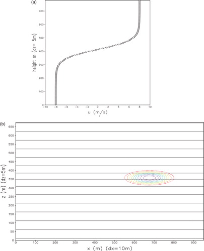
Fig. 5.  (a) Simulated θ at t=320 s with Δtb=0.4 s from θ _δ=1 (Δts=0.01 s, black), θ _δ=4 (Δts=0.02 s, green), θ _δ=16 (Δts=0.04 s, red) and θ _HE-VI(Δts=0.02 s, blue), contour interval is 0.5 K; (b) θ _δ=1 (Δts=0.01 s)−θ _δ=4 (Δts=0.02 s), contours from −0.03 to 0.02 K with interval of 0.005 K; (c) θ _δ=1 (Δts=0.01 s)−θ _δ=16 (Δts=0.04 s), contours from −0.12 to 0.1 K with interval of 0.02 K; (d) θ _δ=1 (Δts=0.01 s)−θ _HE-VI (Δts=0.02 s), contours from −0.02 to 0.03 K with interval of 0.005 K.

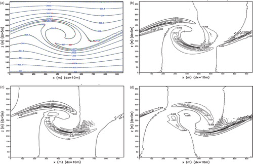
Table 1. Variation of change of the total mass with respect to its initial value as function of time for MFB (δ=16, Δts=0.04 s) and HE-VI (Δts=0.02 s)

	Time (s)
	0	80	160	240	320
[M 16(t)−M(0)]/M(0)	0	2.84057×10^−6	0	7.10142×10^−7	7.10142×10^−7
[M H(t)−M(0)]/M(0)	0	2.13042×10^−6	−7.10142×10^−7	1.42028×10^−6	1.42028×10^−6

4.2. Small Kelvin–Helmholtz waves with Δx=5 m, Δz=5 m and Δts=0.0025 s

The initial x-component wind and the background potential temperature are the same as described in Section 4.1. The amplitude of initial potential temperature perturbation θ′ is −0.4 K, which consists of sine-waves in horizontal with a wavelength of 40 m, and elliptic-type perturbation in vertical with the radius of 120 m, as shown in Fig. 6a. The simulated potential temperature perturbations at t=240 s with Δtb=0.1 s are shown in Fig. 6b from FB with δ=1 (black), δ=4 (green), δ=16 (red) and the HE-VI (blue) with Δts=0.0025 s. The results are almost identical among those three FB simulations. Near to the top of Fig. 6b, the simulation of the HE-VI is slightly different from the FB results. The results show that MFB can produce results of the conventional FB with same Δts, although MFB and HE-VI are intended to apply with a longer Δts than that allowed in the conventional FB (δ=1).

Fig. 6.  (a) Initial background (black) and perturbation θ′ (colour) for Sections 4.2 and 4.3; (b) simulated θ′ at t=240 s from FB with δ=1 (black), δ=4 (green), δ=16 (red) and HE-VI scheme (blue) with Δts=0.0025 s, Δtb=0.1 s and Δx=Δz=5 m. Contour interval is 0.005 K.

4.3. Short waves simulations with Δx=5 m, Δz=5 m with different Δts

Fig. 7a shows the numerical simulations of θ′ at t=240 s with Δtb=0.1 s from FB with δ=1, Δts=0.005 s; δ=4, Δts=0.01 s and δ=16, Δts=0.02 s. They are almost identical. The simulated vertical velocities w (not shown) also converge. The FB (i.e. δ=1) becomes unstable with Δts=0.01 s. The results in Fig. 7a are different from those shown in Fig. 6b (with Δts=0.0025 s), which may be partially due to more smoothing and divergence damping when a small Δts is used in Section 4.2, because the same coefficients are applied to the CReSS model in our simulations.

Fig. 7.  (a) Simulated θ′ at t=240 s from FB with δ=1, Δts=0.005 s (solid line); δ=4, Δts=0.01 s (long dash) and δ=16 Δts=0.02 s (short dash). Contour interval is 0.005 K; (b) θ′ from HE-VI with Δts=0.005 s (dotted line) and Δts=0.01 s (solid line). Contour interval is 0.005 K.

The simulated θ′ from HE-VI with Δtb=0.1 s, and Δts=0.005 and 0.01 s are shown in Fig. 7b. The results from different Δts are almost identical. However, they are significantly different from the simulations from FB shown in Fig. 7a, even with the same time intervals Δts=0.005 s and Δtb=0.1 s. The difference in w between FB and HE-VI is even larger (not shown).

The HE-VI has very effective interaction between p and w, when they are solved in the implicit scheme while u remains constant. This may be valid if Δx>Δz; or Δts is very small; or the variation of the horizontal gradient is small. A large Δts used in Section 4.3 produces significant differences between HE-VI and FB simulations compared with the simulations in Section 4.2. It is likely that the time variation of the horizontal gradient becomes important but is excluded in solving the implicit equation of w and p vertically.

4.4. Thermal bubble

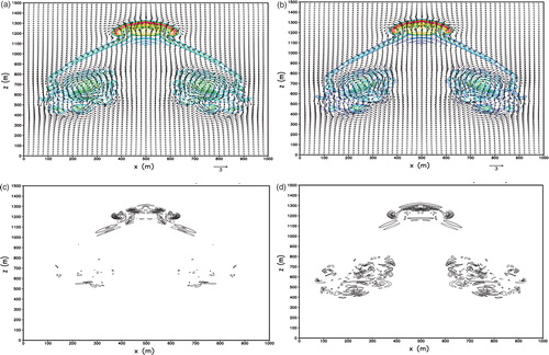
The initial potential temperature of a thermal bubble with a Gaussian profile is shown in Fig. 8a, which was given in eqs. (38) and (39) of Robert (1993). The simulations are carried out using FB with δ=1, Δts=0.008 s; δ=16, Δts=0.03 s and HE-VI with Δts=0.008 s. The Δx=Δz=5 m and Δtb=0.12 s remain the same. The simulated θ and velocity vector at t=6, 12 and 18 min from FB with δ=1 and Δts=0.008 s are shown in Fig. 8b–d. Overall, they are comparable with the simulations of Robert (1993), Hsu and Sun (2001), Chen and Sun (2001), etc., although the detail depends on the numerical schemes and turbulence parameterisation of the models. The simulations at 18 min from MFB with δ=16, Δts=0.03 s; and HE-VI with Δts=0.008 s are shown in Fig. 9a, b, which are close to Fig. 8d. The difference of the simulated θ at 18 min between MFB with δ=16, Δts=0.03 s and FB with δ=1, Δts=0.008 s is between −0.03 and 0.06 K (Fig. 9c, with a contour interval of 0.01 K). The difference between HE-VI and FB is between −0.3 and 0.2 K (Fig. 9d, with a contour interval of 0.04 K). It is noted that both FB with δ=1 and HE-VI become unstable if Δts≥0.01 s, but MFB with δ=16 can use about four times of Δts and reproduces the simulation of conventional FB with Δts=0.008 s. It is noted that Δts=0.03 s instead of Δts=0.032 s is used here because the value of Δtb/Δts should be an integer in CReSS. It is also noted that bubbles have an axis of symmetry, which were also found in the bubble simulations of Hsu and Sun (2001), as well as a 3-D lee-vortex (Sun and Chern, 1994) using TKE-turbulent parameterisation.

Fig. 8.  (a) Initial θ for FB with δ=1, Δts=0.008 s, Δx=Δz=5 m and Δtb=0.12 s. Contour interval is 0.05 K; simulated velocity v and θ(with δ=1) (b) at t=6 min; (c) t=12 min; (d) at t=18 min.

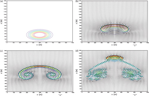
Fig. 9.  Simulated v and θ at t=18 min: (a) with δ=16, Δts=0.03 s; (b) with HE-VI, Δts=0.008 s; (c) θ _δ=16 (Δts=0.03 s)−θ _δ=1 (Δts=0.008 s), contours from −0.03 to 0.06 K with interval of 0.01 K and (d) θ _HE-VI (Δts=0.008 s)−θ _δ=1 (Δts=0.008 s), contours from −0.3 to 0.2 K with interval of 0.5 K.

4.5. Mountain waves

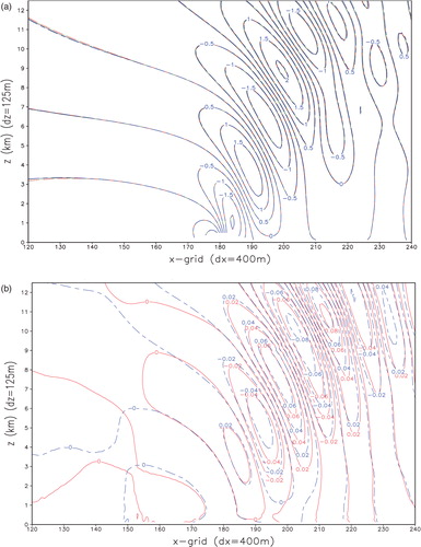
A uniform 10 m s⁻¹ with the buoyancy frequency of 0.01 s⁻¹ flows over a bell-shape mountain with a peak of 500 m and a half-width of 2000 m. The simulated w with Δx=400 m, Δz=125 m and Δtb=10 s, from FB with δ=1, Δts=0.25 s; δ=4, Δts=0.5 s; δ=16, Δts=1.0 s and HE-VI with Δts=1.0 s at t=6000 s are shown in Fig. 10a. They are quite comparable among each other. The difference of simulated w between FB (with δ=1, Δts=0.25 s) and MFB (with δ=16, Δts=1.0 s) at t=6000 s is from −0.06 to 0.08 m s⁻¹ (red); and the difference between FB and HE-VI with Δts=1.0 s is from −0.08 to 0.08 m s⁻¹ (blue) in Fig. 10b. The mountain wave simulations are also comparable with those of Hsu and Sun (2001) and Chen and Sun (2001).

Fig. 10.  Simulated w at t=6000 s with Δx=400 m, Δz=125 m and Δtb=10 s: (a) w _δ=1 (Δts=0.25 s, black), w _δ=4 (Δts=0.5 s, green), w _δ=16 (Δts=1.0 s, red) and w _HE-VI (Δts=1.0 s, blue); (b) w _δ=16−w _δ=1 (red) and w _HE-VI−w _δ=1 (blue), the contour interval is 0.02 ms⁻¹.

The MFB has also been incorporated in the NTU-Purdue NH model to simulate the strong downslope winds and lee-vortices over the Organ Mountains (Haines et al., 2003). Furthermore, a higher-order scheme in space can be easily applied to the terms related to waves, because the MFB is an explicit scheme in both vertical and horizontal directions. On the other hand, the HE-VI scheme uses the second-order scheme in the vertical direction in order to use the tri-diagonal matrix solver.

5. Summary

The MNH model with a parameter δ (between 4 and 16) applied to the continuity equation can suppress the frequency of acoustic waves very effectively with insignificant impact on gravity waves, which enables to use a longer time step. The MNH is simple, in which many numerical schemes can be easily incorporated. The eigenvalues and non-linear model simulations of Kelvin–Helmholtz instability, mountain wave and thermal bubble when FB is applied to MNH (i.e. MFB) show that MFB can reproduce the results of the original NH very accurately and efficiently. It is also found that the simulations from the HE-VI are consistent with those from FB if the time interval Δts is very small, or the time variation of horizontal gradient is not as important as the vertical gradient within Δts. Otherwise, HE-VI simulations can depart from the FB significantly. It is also noted that MFB can use a higher-order scheme in space to simulate LES, turbulence, etc., which requires a fine-resolution in both horizontal and vertical directions.

6. Acknowledgements

We would like to thank the reviewers for their very useful comments as well as the help from Profs. Uyeda and Ohigashi, Kato San and Tsujino San at Nagoya University when the senior author was a Visiting Professor at Hydrospheric Atmospheric Research Center (HyARC), Nagoya University. We also like to thank Mr. Seaman at Purdue Information Technology Center for his help during this study. The computing facilities provided by Nagoya University, Purdue University and Taiwan High Performance Computing Center are also greatly appreciated.

References

- Chen S. H. Sun W. Y. The applications of the multigrid method and a flexible hybrid coordinate in a nonhydrostatic model. Mon. Weather Rev. 2001; 129: 2660–2676.
- Gadd, A. J. 1978. Meteor. Office Tech. Note 48, 8. pp.
- Haines, P. A, Grove, D. J, Sun, W. Y, Hsu, W.-R and Tcheng, S. C. 2003. High resolution results and scalability of numerical modeling of wind flow at white sand missile range. BACIMO (DOD atmospheric science and effects) Conference, September 2003 in Monterey, CA.
- Hsieh, M.-E, Hsu, W. R and Sun, W. Y. 2010. Applications of a three-dimensional nonhydrostatic atmospheric model on uniform flows over an idealized mountain. 2010 Computational Fluid Dynamics Taiwan, Chung-Li, Taiwan, July 29–31. Reprint. P.1–12.
- Hsu W.-R. Sun W. Y. A time-split, forward-backward numerical model for solving a nonhydrostatic and compressible system of equations. Tellus. 2001; 53A: 279–299.
- Klemp J. B. Wilhelmson R. B. The simulation of three-dimensional convective storm dynamics. J. Atmos. Sci. 1978; 35: 1070–1096.
- MacDonald A. E. Lee J. L. Xie Y. The use of quasi-nonhydrostatic models for mesoscale weather prediction. J. Atmos. Sci. 2000; 57: 2493–2517.
- Mesinger, F and Arakawa, A. 1976. Numerical methods used in atmospheric models. GARP Publication Series No. 14, WMO/ICSU Joint Organizing Committee, 64. pp.
- Robert A. Bubble convection experiment with a semi-implicit formation of the Euler equations. J. Atmos. Sci. 1993; 50: 1865–1973.
- Saito K. Nonhydrostatic atmospheric models and operational development at JMA. J. Meteo. Soc. Japan. 2007; 85B: 271–304.
- Sun W. Y. A forward-backward time integration scheme to treat internal gravity waves. Mon. Weather Rev. 1980; 108: 402–407.
- Sun W. Y. Numerical analysis for hydrostatic and nonhydrostatic equations of inertial-internal gravity waves. Mon. Weather Rev. 1984; 112: 259–268.
- Sun W. Y. Conserved semi-Lagrangian scheme applied to one-dimensional shallow water equations. Terrestrial Atmos. Ocean. Sci. 2007; 18(4): 777–803.
- Sun W. Y. Instability in leapfrog and forward-backward schemes: part II: numerical simulation of dam break. J. Comput. Fluids. 2011; 45: 70–76.
- Sun W. Y. Chern J. D. Numerical experiments of vortices in the wake of idealized large mountains. J. Atmos. Sci. 1994; 51: 191–209.
- Sun W. Y. Hsu W. R. Effect of surface friction on downslope wind and mountain waves. Terrestrial Atmos. Ocean. Sci. 2005; 16: 393–418.
- Sun W. Y. Sun M. T. Mass correction applied to semi-Lagrangian advection scheme. Mon. Weather Rev. 2004; 132(4): 975–984.
- Sun W. Y. Sun O. M. T. A modified leapfrog scheme for shallow water equations. J. Comput. Fluids. 2011; 52: 69–72.
- Sun, W. Y, Hsu, W.-R, Chern, J.-D, Chen, S.-H, Wu, C.-C and co-authors. 2009. Purdue atmospheric models and applications. In: Recent Progress in Atmospheric Sciences: Applications to the Asia-Pacific Region. (eds. K. N. Liao and M. D. Chou), World Scientific: Singapore, 496 pp. pp. 200–230.
- Tsuboki, K and Sakakibara, A. 2002. Large-scale parallel computing of Cloud Resolving Storm Simulator. In High Performance Computing. (eds. H. P. Zima et al.), Springer, pp. 243–259.
- Tsuboki, K and Sakakibara, A. 2007. The Seventeenth IHP Training Course (International Hydrological Program). Numerical Prediction of High-Impact Weather Systems. 2 15 December 2007, Nagoya: Japan, 273. pp.