Data assimilation and parametrisation of lakes in HIRLAM

ABSTRACT

When the resolution of numerical weather prediction (NWP) and climate models increases, it becomes more and more important to correctly account for the lake–atmosphere interactions. One possible way to handle lake effects is to use a lake model, which treats the lake surface temperature and ice conditions as prognostic variables. Such a parametrisation eliminates the traditional for NWP need to prescribe lake characteristics based on long-term climate averages. At the same time, new in situ and satellite measurements are becoming available for an operational practice. This offers the possibility to assimilate lake observations into the NWP models. We study the applicability of the prognostic and observation-based approaches and compare both. As a first step towards integrated lake data assimilation and forecasting in NWP, we suggest using the results of the prognostic lake parametrisation as the background for objective analysis (spatialisation) of the lake water surface temperature observations. We run NWP experiments in the Nordic conditions, where the freezing and melting of lakes can significantly influence local weather. Our results indicate that a lake model, usually used in climate studies, works well also in the NWP model even without assimilation of observations. However, it is possible to improve the description of the changing lake surface state by using good observation data. In this case, the lake model provides a better background for the data assimilation than a lake surface temperature climatology.

• data assimilation
• parametrisation
• lake model
• NWP
• lake-atmosphere interactions

1. Introduction

It is widely recognised that lakes modify the local weather and the structure of the atmospheric boundary layer in their surroundings. When the resolution of numerical weather prediction (NWP) and climate models increases, it becomes more and more important to correctly account for the lake–atmosphere interactions. Several recent papers discuss the representation of lakes in NWP and climate models from the point of view of prognostic parameterisations: Mironov (2008), Dutra et al. (2010), Samuelsson et al. (2010), Martynov et al. (2010), Mironov et al. (2010) and Salgado and Le Moigne (2010). Assimilation of lake observations into NWP models has received less attention, perhaps because before now observations were not available over the majority of lakes.

From the point of view of NWP, the most critical periods are the freezing of lakes in autumn and the melting in spring, because frozen and unfrozen surfaces interact differently with the overlying air and are also treated differently in the model. Lakes, especially large and deep ones, retain heat accumulated during the summer until late autumn due to the large heat capacity of water. When cold air masses interact with relatively warm lake water, atmospheric convection and turbulence occur. In such situations, sensible and latent heat are intensively transferred from the water to the air, which may lead to fast cooling and freezing of lakes and enhanced snow precipitation.

In a thick layer of ice, a relatively small amount of heat is transferred by conduction from the underlying water to the air. During winter, lake ice is usually covered by a layer of snow, which tends to insulate more this small heat flux from the atmosphere. The roughness of ice, snow and water surfaces is different, which influences the turbulent fluxes of momentum, heat and moisture in the atmospheric surface layer. The radiative properties, short-wave albedo and, to some extent, long-wave emissivity, are also different for water, dry ice, dry snow, melting snow and melting ice. Snow–ice albedo feedback mechanisms enhance the melting of snow and ice in spring.

In principle, interactions between atmosphere and different types of underlying surface are treated by the different parameterisations in the present-day NWP models. However, for successful parameterisation, it is necessary to correctly describe the distribution of water, ice and snow over water bodies in the model domain. This description can be derived from observations. The water surface temperature is usually obtained by interpolating the sea water surface temperature (SWST) or the lake water surface temperature (LWST) from observational points to the model grid. To our knowledge, there are currently no operational NWP models, which include a full prognostic treatment of sea or lake thermodynamics. Thus, SWST and LWST usually remain unchanged during the forecast. Lake and sea ice concentrations (fractions) may be also obtained from observations. Typically, the prognostic models keep the ice concentration constant between the analysis times.

One of the main differences between NWP and climate model is in the use of data assimilation. An NWP model starts new short-range forecasts several times a day from an initial state based on fresh observational information, while a climate model utilises measurements only for calibration and validation. The role of a prognostic lake parameterisation is also different in NWP and climate models. Climate models rely only on a parameterisation while NWP models may benefit from the use of in situ or space-borne lake measurements as a means of improving the parameterisation result. In order to do this, advanced methods of data assimilation would need to be applied to avoid disturbing the balanced state of the atmospheric model with observations, which are local and therefore discontinuous. In the analysis of LWST, a prognostic lake parametrisation coupled to the NWP model may play an important role in the future by providing background information. Over lakes for which there are no observations, the application of such a prognostic parameterisation may replace the usage of climatological information.

Regular space-borne information about the state of lake surface is, in principle, available for assimilation in NWP models, although these measurements were not used in this study. For example, the lake surface temperature and the ice fraction are derived from the Moderate Resolution Imaging Spectroradiometer (MODIS) flying on board NASA's Aqua and Terra satellites (http://modis.gsfc.nasa.gov). Kheyrollah Pour et al. (2012) compared them with in situ measurements and also simulations done using 1-D lake models. Ice conditions are measured over Lake Vänern and Lake Vättern, which are large Swedish lakes. These measurements are included in the Baltic Sea ice chart (Grönvall and Seinä, 2002), which is presently used by the operational HIgh Resolution Limited Area Model (HIRLAM, Undén et al., 2002) NWP model at the Finnish Meteorological Institute (FMI). Information on snow covering lake ice in spring is derived from MODIS and AVHRR data in the Finnish Environment Institute (SYKE), by applying the methods described by Luojus et al. (2006). In principle, this information also may be used in NWP models, although at present there are no methods to assimilate it.

The present study focuses on data assimilation and its interaction with the prognostic lake parameterisation in an NWP model. Our main focus is on Nordic spring and autumn conditions. We run various HIRLAM experiments for the period of November 2009–May 2010. In these experiments, in situ measurements of the surface temperature of lakes (but not satellite observations) have been analysed in a simplified way. We want to contribute to the ongoing discussion concerning questions such as: How much we can benefit from observations of lake surface temperature alone, without also including the prognostic parameterisation? Would the application of a prognostic lake parameterisation make assimilation of observations less important? Do the results of the analysis or of the parameterisation of the lake surface state really influence the numerical weather forecasts on local or large scales?

This study continues the work reported by Eerola et al. (2010). Compared to the earlier study, we have advanced in several aspects. Firstly, we obtained more in situ observations of the surface temperature of lakes and we used them in the analysis. Secondly, in the analysis, we used the optimal interpolation method instead of successive corrections. Thirdly, the LWST field produced by the prognostic lake parameterisation was used as the background state for analysis of observations. Fourthly, we utilised a model climatology of prognostic lake variables developed by Kourzeneva et al. (2012). Finally, we also studied the behaviour of HIRLAM over lakes during the snow/ice melting period.

We report on our recent experiments and discuss problems detected. We present this material in the hope of supporting those applying and developing lake prognostic parameterisations in NWP models, where the use of observations and data assimilation are essential.

2. Observations, data assimilation and the prognostic model

In this section, observations, data assimilation methods and the prognostic parameterisation are presented at a general level. Section 3 describes the use of these methods in our experiments. In HIRLAM, the fraction of lakes in each grid box and the lake depth are included in the description of the physiography. The temperature of the lake water surface and the fraction of ice in each grid box may be obtained from the prognostic lake model or from the analysis of surface observations. The lake model predicts also the characteristics of the lake water temperature profile, the thicknesses of ice and snow layers and the temperatures of ice and snow.

2.1. Observations and climate data

A common practice in NWP models is to use analysed SWST, based on ship and satellite observations. Very often climatological values for lakes are obtained by extrapolation of SWST climatology from the nearest ocean (in this paper, we will refer to these data as ‘ocean-derived’ climatology). A better solution is to apply climatological values obtained from measurements.

In HIRLAM, for LWST pseudo observations are used instead of observations. To produce them, climatological values from different sources are used. For example, in the previous operational version of HIRLAM, a so-called ‘Finlake’ climatology was used over Finland. This dataset is derived from historical time series of the surface water temperature combined with the freezing and break-up dates of 10 lakes in Finland (Eerola et al., 2010). Also in the previous operational version of HIRLAM, the European Centre for Medium Range Weather Forecasts (ECMWF) analysis data are used as pseudo observations. They contain the surface temperatures of lakes, based on time-lagged long-term averages of the simulated screen-level temperature (Gianpaolo Balsamo, personal communication). These data cover all large lakes, including those in the Scandinavian, Baltic and Karelian areas. Although theoretically the use of climatological information in the form of pseudo observations is not correct (see Section 2.2 for more details), this is a common operational practice.

In situ observations over large lakes also exist and may be used by NWP models. The SYKE has 32 regular lake water temperature measurement sites in Finland. The temperature of the lake surface water is measured every morning at 8:00 am local time close to the shore and 20 cm below the water surface. The measurements are either automatic (13 stations) or manual and are performed only in ice-free conditions. At SYKE, a statistical moving-average-type lake surface water temperature model (Elo and Koistinen, 2002) is developed (it uses a short-wave radiation index as an additional predictor). This model works operationally using the latest observations to calibrate it. It works well only when recent observations are available. During the melting period in spring, the error associated with the statistical fit may be large, because no LWST observations are available when the lake is covered with ice.

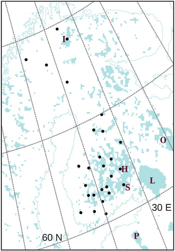
In this study, we used SYKE observations from 27 sites over Finland, backed up with the statistical model (Fig. 1). When available, present or previous day observations are used; otherwise the value from the statistical fit is applied. These observations only cover Finland, while typically a HIRLAM domain is significantly larger. These observations are also used by the operational version of HIRLAM since December 2010, replacing the Finlake climatology.

Fig. 1.  Location of 27 SYKE lake temperature measurement stations, shown with the grid box lake fraction in the operational setup of HIRLAM with a horizontal resolution of 16.5 km. The blue colour indicates that more than 5% of the grid square is covered by lakes. The letters denote the lakes mentioned in this study: I – Lake Inari, H – Lake Haukivesi, S – Lake Saimaa, O – Lake Onega, L – Lake Ladoga, P – Lake Peipsi.

In the operational version of HIRLAM, information about (sea) ice cover is obtained from different products, such as the ECMWF analysis. This information is represented in the form of pseudo observations of the water surface temperature using simple coding rules. If ice is detected in a product, the water surface temperature pseudo observation gets the value less than some threshold. For lakes, this coding rule is also applied. In this study, neither lake ice cover measurements nor satellite observations of LWST were used.

2.2. Methods of analysis of water surface variables

Over water bodies in HIRLAM, there are two analysed surface variables: the surface temperature of the water and fraction of ice within the grid box. In the surface data assimilation, the SWST and LWST are treated in a similar manner. Both for SWST and LWST, analysis means the horizontal interpolation of the observed values to the latitude–longitude grid of HIRLAM. Analysis is performed using optimal interpolation (Gandin, 1965). In optimal interpolation, a background field (usually a short-range model forecast or a previous analysis) is combined with nearby observations. The weight of an individual observation is calculated using autocorrelation function, depending on the horizontal distances. Elevation differences are also possibly included. The weight depends also on the prescribed observation and background error standard deviations.

In this study, lake observations were assumed to have the observation error standard deviation of 1.5c, while the background error standard deviation for SWST and LWST was assumed to be 1 °C. Autocorrelation function was dependent on the horizontal distance only, although in principle, also other factors which describe lake properties (e.g. lake depth) should be taken into account.

A quality check for the observations is made by comparing them to the background field and to neighbouring observations. The difference between the observation and the background value at the observation point is scaled using the observation and background error standard deviations. If the scaled difference is larger than some threshold value, the observation is rejected. Another check is made using surrounding observations. The check applies optimal interpolation of the nearby observations to the observation point in question, and then estimates if the scaled difference between the actual and interpolated value is realistic. It is difficult to set objective criteria for the quality control. In our experiments, quite a liberal approach was adopted; only observations which deviated from the reference by more than 10 °C were rejected.

HIRLAM model runs, including analysis and forecast, start four times daily (at 00, 06, 12 and 18 UTC). The background is provided by the 6-h forecast of the previous cycle. When the prognostic lake parameterisation is not applied, LWST remains unchanged during the forecast, thus the background in fact stands for the previous analysis. Surface observations are introduced in each cycle, even though they may be valid for the whole day. Pseudo observations, which represent climatological information for lakes (ECMWF LWST fields, Finlake data), are interpolated to the model grid along with the real observations. This introduces inconsistency and gives the climatology a too-large weight. We will show later that the use of a prognostic lake model makes pseudo observations unnecessary.

As traditionally ice cover observations are represented in the form of the water surface temperature pseudo observations, the fraction of ice over the sea and lakes is diagnosed then from the analysed SWST and LWST. A grid box over a lake (or over the Baltic Sea or in any coastal zone) is assumed to be completely ice-covered when the temperature of the water is less than 272.65 K, and where the temperature of the water is above 273.15 K there is no ice. Between these temperature thresholds, the fraction of ice changes linearly. This procedure, although common in NWP models, represents a very simplified way of handling ice cover when it is not directly derived from (satellite) measurements.

If the prognostic lake parameterisation is not applied in HIRLAM, SWST and LWST remain unchanged during a forecast. (However, the ice thickness and the temperature of the ice surface are predicted by the parameterisation of ice.) To provide the seasonal change and to guarantee that the LWST does not drift to an unrealistic state when observations are missing, the background field of LWST is relaxed towards climatology. For this, a gridded ‘ocean-derived’ climatology is used. Thus, over lakes where observations are not available, these artificial climatological values determine the analysed field. In case the prognostic lake parameterisation is applied (see Section 2.3), the state of the lake surface is provided by this parameterisation and used as the background for the analysis. In this case, relaxation towards climatology is unnecessary.

In the first forecast-data assimilation cycle, the surface analysis is replaced by the climatological values of the surface variables. For LWST and the ice cover over the lakes, the ‘ocean-derived’ climatology is used.

2.3. Implementation of the prognostic lake model FLake into HIRLAM

The Freshwater Lake model (FLake) (Mironov, 2008; Mironov et al., 2010) was originally included as a parameterisation scheme in the HIRLAM forecasting model by Kourzeneva et al. (2008). Eerola et al. (2010) discuss the specific features of the implementation of FLake into HIRLAM. In the present study, a first version of the integrated HIRLAM forecasting-data assimilation system with FLake was built. Integration means that (1) the description of lake properties (fraction of lakes within a grid box, lake depth) and a model climatology of FLake prognostic variables was included; (2) during the forecast, FLake is coupled to the atmospheric model and (3) the prognostic LWST given by FLake provides the background for analysis over the lakes.

As a first step towards the integrated lake data assimilation system, a simple concept of peaceful coexistence between FLake prognostic parametrisation and lake analysis block was developed (see Fig. 2). This concept means that FLake predicts the mixed layer temperature, the mean water temperature, the bottom temperature, the ice temperature, the snow temperature, the mixed layer depth, the ice thickness and the snow thickness. Based on the FLake prognostic variables, the surface temperature over the lake and the fraction of ice (1 or 0, as a lake grid box is considered either ice-covered or free of ice) are diagnosed. At each time step of the HIRLAM forecast, FLake is driven by the atmospheric radiative and turbulent fluxes provided by the physical parameterisations in HIRLAM, which combine the atmospheric variables over lakes with the lake water surface properties described by FLake. The predicted lake surface properties provide the background for the next analysis cycle, when new observations are introduced into the model.

Fig. 2.  Schematic representation of the concept of peaceful coexistence between lake analysis and lake parameterisation by FLake.

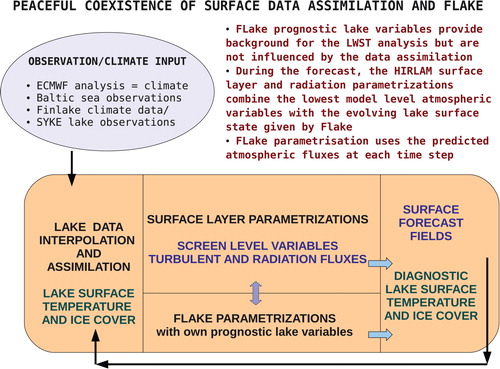
With new observations, the analysed LWST and ice fraction may differ from the background provided by FLake. However, FLake continues to integrate the prognostic equations in time directly from the results of the previous forecast cycle, omitting the analysis. It works in the same way as it works in a climate model, where the time integration is not interrupted by the assimilation of new information. The fields of prognostic lake variables are not influenced by the data assimilation. In fact, the analysed LWST and ice fraction do not influence the atmospheric forecast either, because FLake (but not the analysis) provides the lake surface state during the forecast. The LWST and the ice fraction provided by the analysis can be considered as an independent output from HIRLAM, perhaps useful for applications.

In our experiments, we used the snow-on-ice parameterisation in FLake [in Eerola et al. (2010), the snow-on-ice block was switched off]. We introduced a constant snow density and modified the snow and ice albedoes, as suggested by Semmler et al. (2012). For the radiation transfer in water and snow, the light extinction coefficient was set to values representing turbid lake water (5 m⁻¹) and fully opaque ice and snow (10⁷ m⁻¹).

The bottom sediment parametrisation in FLake was inactive. Despite application of a zero flux lower boundary condition, for boreal lakes there is no drift of the bottom temperature in FLake. This is because during the freezing period, the bottom temperature is kept close to the maximum water density point, see Kourzeneva et al. (2012) for more details and explanations.

For our experiments, information about lake depth from the lake database for NWP by Kourzeneva (2010) was combined with the lake fraction in the HIRLAM physiography description [see Undén et al. (2002) for details]. For the very first, so-called ‘cold’ start of FLake, climatological values of the prognostic lake variables were retrieved from the model lake climatology dataset developed by Kourzeneva et al. (2012). This information is required by FLake in order to start prognostic calculations at any time of the year. In HIRLAM, the model lake climatology is used only for the ‘cold’ start but not for relaxation of the analysed LWST towards climate values or for any other purposes.

3. Experiment setup

Three main series of HIRLAM experiments (CLI, ANA and FLK) were performed over a Nordic domain (Table 1). ECMWF and Finlake pseudo observations (both representing climatology) were assimilated in the climatological experiment (CLI). Over lakes, real observations were absent and prognostic parameterisation was not applied. The background for the LWST analysis was provided by the previous analysis, which was relaxed towards the ‘ocean-derived’ climatology. The same ‘ocean-derived’ climatology was used instead of the analysis in the first forecast cycle. This setup was used in the FMI operational HIRLAM model before the year 2010.

Table 1. Definition of the HIRLAM experiments

Experiment	FLake	Observations	Lake initialisation	Comment
CLI	No	ECMWF^b+Finlake	LWST^c climatology
ANA	No	SYKE^a+ECMWF^b	LWST^c climatology
FLK	Yes	SYKE^a only	LWST^c+in-lake^d climatology
SYK-c	Yes	SYKE^a+ECMWF^b	LWST^c+in-lake^d climatology	Cold start
SYK-w	Yes	SYKE^a+ECMWF^b	Previous experiment	Warm start

^aObserved LWST over 27 lakes in Finland.

^bClimatological pseudo observations over the largest lakes.

^cFor analysis.

^dFor FLake.

In the analysis experiment (ANA), SYKE observations were used instead of Finlake pseudo observations. ECMWF pseudo observations were used, but no lake prognostic parametrisation was applied. Background and relaxation were treated as in the CLI experiment. Thus, the only difference between the CLI and ANA experiments was in the use of SYKE observations. This setup was used in the operational HIRLAM system at FMI until February 2012.

The prognostic experiment (FLK) combined FLake parameterisation with SYKE observations using the concept of peaceful coexistence. Pseudo observations and relaxation of the analysis to the ‘ocean-derived’ climatology were excluded. The lake model climatology dataset was used for the ‘cold’ start of the prognostic lake variables. No SYKE observations were available over the large lakes, for example, over Lake Ladoga, Lake Onega, Lake Peipsi, Lake Vänern and Lake Vättern. Hence, the FLK experiment showed over these lakes how LWST analysis and FLake behave without observations and influence of climatology. We suggested that this setup for the present reference version of HIRLAM – version 7.4, which is prepared for operational use at FMI from February 2012.

Experiments CLI, ANA and FLK were started from 1 November 2009. Forecast-data assimilation cycles run until 31 May 2010. In addition, two short 4-week experiments (SYK-c and SYK-w) were performed starting from 20 June, 2011, in order to study the impact of the model lake climatology on the HIRLAM forecasts. In both experiments, FLake and SYKE observations were included. The setup for both was similar to the FLK experiment setup. The difference between them was that SYK-c used initial values of the prognostic lake variables given by the lake model climatology (‘cold’ start), while SYK-w continued the time integration using results of a previous experiment (‘warm’ start).

For all experiments, we used HIRLAM version 7.4beta1 with a horizontal resolution of 6.8 km over a Nordic experiment domain (as in Eerola et al., 2010) and 65 levels in vertical between the surface and the 10 hPa level in the atmosphere. For the upper-air data assimilation, the 3-D variational method was used. Four data assimilation – forecast cycles with the forecast lead time of 9 h started at 00, 06, 12 and 18 UTC every day. The lateral boundary conditions for the atmospheric model were provided by the fields of ECMWF analysis.

4. Experiment results

In this section, we present and analyse snapshots of the experiment results. A 15th December, 2009 case study focuses on lake freezing. An example of Lake Haukivesi reveals differences between model experiments in spring-time lake melting. Results of the summer experiments highlight a problem related to the lake model climatology. Finally, screen-level temperature validations are presented and discussed.

4.1. The 15th December, 2009 case study

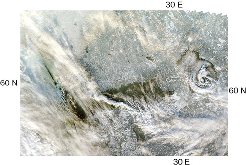
In mid-December 2009, a strong cold air outbreak occurred over the unfrozen Lake Ladoga and the Gulf of Finland. In the MODIS Aqua satellite image (Fig. 3, from the site http://lance.nasa.gov/imagery/rapid-response/subsets/), North–West to South–East convection lines can be seen over the Baltic Sea, while a mesoscale cyclone developed over Lake Ladoga. HIRLAM could handle the evolution of convection and forecast these cloud formations, but only when the lake surface state was correctly described (experiment results are not shown).

Fig. 3.  MODIS Aqua view over Gulf of Finland (in the middle) and Lake Ladoga (on the right) in the afternoon on 15 December 2009. Note the mesoscale cyclone over Ladoga and convection lines over Gulf of Finland.

A comparison of the ice fraction suggested by the main experiments (CLI), (ANA) and (FLK) (Fig. 4) revealed that the climatological (CLI) and analysis (ANA) experiments, without FLake but using ECMWF pseudo observations (based on climatology) over Lake Ladoga, assumed that the entire lake was frozen. In fact, in these experiments, Lake Ladoga froze at the beginning of December. A setup with FLake but without the ECMWF data (FLK) correctly indicated that the largest part of Lake Ladoga was still unfrozen. In this experiment, the entire lake froze during the first half of January, which corresponded well to the available MODIS satellite images (not shown).

Fig. 4.  Fraction of lake ice in a grid square (0–1) at 06 UTC on 15 December, 2009, according to the analysis by the (a) CLI, (b) ANA and (c) FLK experiments. The grid squares where the lake fraction is greater than 25% are shown.

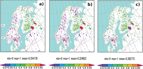
In all experiments, for Lake Ladoga the difference between the analysis and background in terms of LWST and ice fraction was insignificant. The SYKE observations do not cover Lake Ladoga, and the nearest lakes for which there are SYKE observations are too far away to influence Lake Ladoga grid points. The same is true for the Finlake pseudo observations used in the CLI experiment. In CLI and ANA, the climate-based pseudo observations from ECMWF considered the temperature of Lake Ladoga to be below the freezing point. Thus, using the prognostic parameterisation based on FLake even without data assimilation led to the best results over Lake Ladoga.

For Finland, the difference between the ANA and CLI experiments was small. This is because both the SYKE observations and Finlake climatology indicated that the lakes in Finland were mostly frozen at that time. The results of FLK over Finland also agreed with those of ANA and CLI. For the rest of the domain, ANA and CLI experiments used the same climate-based pseudo observations and relaxation to the ‘ocean-derived’ climatology. Thus, outside Finland, much larger differences appeared between the ANA and CLI experiments on the one hand, and the FLK experiment on the other hand. The large Karelian lakes, including Lake Onega, behaved like Lake Ladoga; according to the climatology they were frozen but according to FLake they were unfrozen, which was more realistic. The case of Scandinavian, Baltic and Kola Peninsula lakes was the opposite; they were unfrozen according to the climatology but were frozen north of 60 N according to FLake. In this case, FLake alone also produced the best results. Hence, there seems to be no benefit from using the climatological LWST information in addition to the lake model.

4.2. Freezing and melting of Lake Haukivesi

We compared the observed and simulated freezing and melting dates of Lake Haukivesi during 2009–2010. Lake Haukivesi is a large lake in South-eastern Finland (see Fig. 1 for the location), with lake centre coordinates of 62.11N, 28.39E, a surface area of 562 km² and a mean (maximum) depth of 9 m (55 m). According to SYKE visual observations (Table 2), the whole lake was frozen on 14 December, 2009, and the ice broke up on 4 May, 2010. The last autumn in situ measurement indicated that the water surface temperature was already close to 0 °C on the 5th of November. The first spring measurement showed a temperature of 5 °C on 5 May, 2010. Well before this, on 2 April, the SYKE statistical model indicated a temperature rise above 0 °C. Note that the water temperatures are measured close to the shore while the visual observations attempt to estimate the ice cover over the whole lake.

Table 2. Ice freezing and break-up dates of Lake Haukivesi in 2009–2010

	Freezing	Break-up
Observed
SYKE LWST > 0°C	4 December	5 May/2 April^a
SYKE visual	14 December	4 May
Simulated
CLI analysed	26 November	5 May
ANA analysed	2 December	2 April
FLK analysed	5–7 December	2 April
FLK predicted	4 December	15 April

^aSYKE statistical model.

The observed temperatures and the temperatures estimated by SYKE statistical model were used by the ANA and FLK experiments and were all accepted by the model's quality control. No other observations or pseudo observations were available over Lake Haukivesi. The closest neighbouring lakes with observations are located more than 100 km from Lake Haukivesi and thus weakly influence the result of analysis there. The visual observations of ice cover were used for validation only.

Table 2 shows that the freezing dates according to the ANA (with analysis but without FLake) and FLK (with analysis + FLake) experiments were close to each other and to the date indicated by the LWST observations, but were too early compared with the visual observations (as one could expect).

The situation in spring is more problematic; the melting of Lake Haukivesi occurred already in early April in the ANA and FLK experiments. This was because in the analysis the too warm SYKE statistical estimate was used instead of the observations which had not yet begun. We may conclude that only the measurements, but not the statistical model, should be applied during spring. In addition, it seems to be useful also to utilise the visually observed freezing and break-up dates for the ice cover analysis.

In the forecast part of the FLK experiment, FLake suggested a break-up date of the 15th April independently of observations. This was a few weeks later than estimated by the ANA and FLK analysis, but was still 3 weeks earlier than visually observed. This points to a need to test more wintertime FLake parameterisation and to develop data assimilation system for lakes. In the FLK experiment, the HIRLAM analysis and forecast showed a different state for Lake Haukivesi during 2 weeks in spring. This was due to the peaceful coexistence approach (as described in Section 2.3). Only the forecasted lake state was used by the atmospheric model. The improved background did not lead to a better analysis here because the erroneously estimated observations were dominant.

4.3. Problem of initialisation at the ‘cold’ start

Operational NWP model simulations or modelling experiments must be able to start at any time of the year. When FLake is applied, a model lake climatology is needed in order to provide realistic initial values for the prognostic lake variables, namely the characteristics of the water, ice and snow temperature profiles and thicknesses of ice and snow. Our basic experiments started at the beginning of November, when most of the northern lakes are in a well-mixed state and are quite correctly described by the model lake climatology (Kourzeneva et al., 2012).

The situation in spring and summer was more complicated. Our first attempts to start FLake experiments in spring, when lakes are covered by ice, were unsuccessful as the ice never melted. Additional experiments (SYK-c and SYK-w) were performed to study the problem. SYK-c was initialised using the model lake climatology. SYK-w was continued from previous experiment, which started in the autumn.

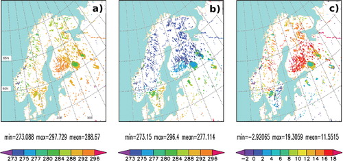
The lake surface (water or ice) temperature suggested by FLake, just after the start of the experiments, was more than 10 °C colder in SYK-c than in SYK-w (Fig. 5). In SYK-c, thick ice covered the Scandinavian lakes above 63 N, while there was no ice in SYK-w, which was correct (figure not shown). This means that the ice cover in the lake model climatology is unrealistic for northern latitudes in spring. In their current form, these data do not provide a sufficiently good starting point for NWP simulations. In the SYK-c experiment, it took over 2 weeks of simulation to reach realistic analysed values of lake temperatures over lakes where observations were available. However, by the middle of July, the average LWST over all of the lakes was still more than 2 °C colder in SYK-c compared with SYK-w.

Fig. 5.  Lake surface temperature (K) on 20 June, 2011, at 06 UTC according to the parameterisation by FLake in (a) SYK-w, (b) SYK-c and (c) their difference. Lakes are masked out as in Fig. 4.

Another problem, which is related to snow on ice, was revealed comparing the lake climate fields and experiments started in autumn (e.g. FLK). In the FLake setup used to develop the lake model climatology, the snow block was switched off. Hence, in this dataset, there is no snow on lake ice, and the snow temperature is set to be identical to the ice temperature. The results of HIRLAM experiments, which do apply the snow-on-ice block in FLake, depend on the starting time. In the case of an autumn starting time, the atmospheric model will produce snowfall, which will be accumulated on lake ice and will be handled by FLake. Until the early spring, presumably the maximum thickness of the snow layer will be reached. During the entire snow season, the presence of snow will also influence the growth of ice in FLake. On the contrary, in a spring experiment starting from the model lake climate dataset, perhaps in winter on the time of maximum actual snow depth, snow will start accumulation from zero. In practice, in such an experiment, a snow depth has no chance to reach realistic values before melting. The break-up date will be different in the two experiments due to the different snow cover. Thus, it is desirable to include estimates of the climatological snow depth into the lake model climatology dataset.

4.4. Validation of the screen-level temperature

We compared six-hour forecasts with synoptic observations (SYNOP) at all stations in Northern Scandinavia, in the Baltic area and in North-western Russia (WMO, World Meteorological Organisation, blocks 01, 02, 26, 22). A monthly systematic error (bias) between the forecasted and the observed screen-level temperature was calculated. All of the experiments showed a cold bias of −0.32 to −0.65 °C in April–May and in November–December, while in the middle of winter there was almost no bias. According to operational verification (available on www.hirlam.org), the small cold bias in short-range forecasts is typical in the current version of HIRLAM, and not related to the handling of lakes in particular. Note also that these general verification scores smooth the results, for example, by combining a warm bias of the coldest temperatures with a cold bias of the warmest temperatures. For other predicted variables, we found no significant differences in the verification scores between our experiments.

In our experiments, the influence of different kinds of lake data assimilation and parametrisation on verification scores was minor. The smallest cold bias in November occurred in the ANA experiment, where the Swedish and Norwegian lakes were incorrectly not frozen while the state of the Finnish lakes was more correctly described (based on observations). Locally, large positive bias values were noticed close to the unfrozen Swedish and Norwegian lakes. In spring, the largest cold bias was shown by the CLI experiment, where many lakes were frozen for too long due to the use of the cold Finlake pseudo observations and relaxation to ‘ocean-derived’ climatology. On the contrary, in the FLK and ANA experiments, some of the Finnish lakes were too warm as a result of using the SYKE statistical estimates (see discussion in Section 4.2).

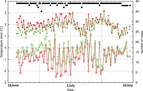
The large difference between the additional cold and warm start experiments of SYK-c and SYK-w also showed up in the validation (Fig. 6). Just after the start of the experiments, the cold bias of SYK-c over Finland was typically one degree larger than in SYK-w, and the RMSE was half a degree larger. Within 2 or 3 weeks, the screen-level verification scores of two experiments converged and were equal during the last week. In both experiments, the bias tends to be largest during the night and morning (00 and 06 UTC).

Fig. 6.  Time-series of bias (lower curves with squares) and RMSE (upper curves with circles) of the predicted grid-average screen-level temperature of SYK-c (red) and SYK-w (green) experiments against 39 SYNOP stations in Finland between 20 June and 15 July, 2011. The number of cases is depicted by the black line. Left y-axis: temperature in °C, right y-axis: number of cases, x-axis: date. Statistics are based on the initialised analyses and 6-h forecasts started at 00 and 12 UTC every day. Note that the initialised analysis contains values diagnosed from FLake, and not the analysed temperatures.

5. Discussion

From the point of view of data assimilation, there are different types of lakes in HIRLAM: (1) the largest lakes where climatological surface temperature data are available from ECMWF, for example, Lake Ladoga, Lake Saimaa, Lake Inari, Lake Peipsi, Lake Vänern and Lake Vättern in our experiment domain; (2) the 27 Finnish lakes, for which SYKE observations are available, and ECMWF data exist also for some of them; (3) lakes close to the lakes where observations exist (and influenced by the neighbours); (4) lakes where only ‘ocean-derived’ climatology is available for LWST; and (5) lakes which are too small or incorrectly described by the model physiography.

In any operational NWP domain most lakes belong to the category where no observations are available. The Freshwater Lake model (FLake) parameterisation may work either alone or in peaceful coexistence with spatialised observations for the lakes of all categories except the poorly defined ones. Realistic results seem to be possible when FLake is applied without assimilation of observations and climatological data. Based on the present study, we suggest replacing the use of all climate-based lake information with the prognostic parameterisation by FLake. This means excluding the Finlake and ECMWF pseudo observations as well as the SYKE statistical LWST model estimates, at least during the melting period. Application of a lake parameterisation also means that relaxation of the analysis towards the ‘ocean-derived’ climatological LWST becomes unnecessary.

More work is needed to find and implement new in situ and space-borne observations of lake temperature and ice cover for real-time use in operational NWP practice. Over our Nordic domain, priority should be given to satellite observations, mainly over the largest lakes. MODIS-based temperature and ice cover data might be used. Assimilation of visual observations of ice freezing and break-up dates should be considered. For the analysis methods, improved autocorrelation functions need to be constructed for the optimal interpolation. These might take into account lake depth (in addition to horizontal distance and possibly altitude difference), which is presumably the most important parameter influencing lake thermodynamics.

When testing the concept of the peaceful coexistence of lake observations and the prognostic lake model, we gained an insight into the needs for lake data assimilation in NWP models. Currently, observations in fact do not influence the results of prognostic lake parameterisation and the atmospheric forecast. To ensure that the observed LWST consistently influences both FLake and the atmospheric model, advanced data assimilation methods are needed.

To initialise an experiment or an operational forecast by an NWP model where FLake is applied, climatic values of the lake prognostic variables are needed. They are provided by the lake climatology for NWP (Kourzeneva et al., 2012). We noticed that the ice thickness in this dataset seems to be overestimated during spring in Northern Europe. The same conclusion was made and discussed by Kourzeneva et al. (2012). Another problem is that in the model lake climatology, an estimate of the snow depth over lake ice is currently not given. An improvement of the dataset especially for springtime would be beneficial for NWP applications.

6. Conclusions and outlook

To summarise, we give preliminary answers to the questions posed in Section 1. The first question: How much we can benefit from observations of lake surface temperature alone, without including a prognostic parameterisation? We need a good background to be able to optimally use information from the observations. Too large differences between observed and simulated lake surface temperatures may lead to the rejection of the observations in the data assimilation. The best background seems to be attained by the prognostic lake parameterisation. Good observations by themselves may also improve the analysis of LWST and lake ice cover. However, in this case, (1) an adjustment of methods of the optimal interpolation to LWST is needed and (2) the quality of the LWST climatology used for relaxation gains more importance. Currently, in situ measurements of lake parameters are sparse and only few space-borne observations used to cover the rest of the lakes. For these reasons, we would suggest the application of the prognostic lake parameterisation in all cases.

The second question was: Would the application of a prognostic lake parametrisation make the use of observations less important? Prognostic lake parameterisation leads to a better description of the surface state of the lake, especially for lakes where observations are unavailable. Currently, such lakes represent the majority of lakes treated in NWP models. In this case, the parameterisation, which depends on the current state of the atmosphere, replaces the lake climatology, which only reflects the average conditions. This should improve the results. To make the prognostic parameterisation more realistic, especially for winter conditions and melting of ice, improvements of FLake seem to be desirable.

For lakes where observations are available the lake parameterisation provides the background for the analysis. However, in the peaceful coexistence setup, the observations are not yet tied to the parameterisation. In this study, we saw large differences between the analysed and predicted LWST fields in spring but not in the autumn. Further development of advanced lake data assimilation is necessary.

The third question was: Do the analysis and parameterisation of the lake surface state influence local or larger-scale numerical weather forecasts? Until now, we have seen only local effects related to near-surface temperatures, which may also show up in the verification. There are cases where the lake surface state affects the local weather, for example, the Lake Ladoga mesocyclone case discussed in Section 4.1. With the increase in NWP model resolution, more attention is paid to the accuracy of local weather forecasts. Thus, more accurate representation of lakes in NWP models is increasingly important even if significant larger-scale effects are not detected. In addition, local effects may be long-lasting and dependent on the season. More studies, including forecasts with longer lead times than used here, are needed to quantify the importance of lake effects on predicted temperature, precipitation, cloudiness and wind.

7. Acknowledgements

We thank Dr. Emily Gleeson for the careful reading and suggestions for the language revision of this manuscript. Comments by the anonymous reviewers helped to improve the contents and readability of the manuscript. The support of this study by the European Space Agency project STSE – North Hydrology is gratefully acknowledged.

References

- Dutra, E, Stepanenko, V. M, Balsamo G, Viterbo P, Miranda, P. M. A and co-authors. 2010. An offline study of the impact of lakes on the performance of the ECMWF surface scheme. Boreal Env. Res. 15, 100–112.
- Eerola K. Rontu L. Kourzeneva E. Shcherbak E. A study on effects of lake temperature and ice cover in HIRLAM. Boreal Env. Res. 2010; 15: 130–142.
- Elo, A and Koistinen, A. 2002. Evaluating temperature of lake surface and lake evaporation in Mäntyharju watershed area. In: XXII Nordic Hydrological Conference, Röros. NHP Report No. 47. Nordic Hydrological Programme, Tapir trykkeri, 417–426.
- Gandin, L. 1965. Objective Analysis of Meteorological Fields. Gidrometizdat, Leningrad. Translated from Russian, Jerusalem, Israel Program for Scientific Translations, 242 pp.
- Grönvall, H and Seinä, A. 2002. Satellite data use in Finnish winter navigation. In: Operational Oceanography: Implementation at the European and Regional Scales – Proceedings of the Second International Conference on EuroGOOS, 11–13March1999, Rome, Italy (eds. N. C. Flemming et al.). Elsevier, pp. 429–436.
- Kheyrollah Pour, H, Duguay, C. R, Martynov, A and Brown, L. C. 2012. Simulation of surface temperature and ice cover of large northern lakes with 1-D models: a comparison with MODIS satellite data and in situ measurements. Tellus. 64A, 17614, doi: 10.3402/tellusa.v64i0.17614.
- Kourzeneva E. External data for lake parametrisation in Numerical Weather Prediction and climate modelling. Boreal Env. Res. 2010; 15: 165–177.
- Kourzeneva, E, Martin, E, Batrak, Y and Le Moigne, P. 2012. Climate data for parameterization of lakes in NWP models. Tellus. 64A, 17226, doi: 10.3402/tellusa.v64i0.17226.
- Kourzeneva, E, Samuelsson, P, Ganbat, G and Mironov, D. 2008. Implementation of Lake Model FLake into HIRLAM. HIRLAM Newsletter. 54, 54–64. Available from HIRLAM-A Programme, c/o J. Onvlee, KNMI, P.O. Box 201, 3730 AE De Bilt, The Netherlands. Online at: http://hirlam.org.
- Luojus K. Pulliainen J. Metsämäki S. Hallikainen M. Accuracy assessment of SAR data-based snow covered area estimation method. IEEE Transactions in Geoscience and Remote Sensing. 2006; 44: 277–287.
- Martynov A. Sushama L. Laprise R. Simulation of temperate freezing lakes by one-dimensional lake models: performance assessment for interactive coupling with regional climate models. Boreal Env. Res. 2010; 15: 143–162.
- Mironov, D. V. 2008. Parameterization of lakes in numerical weather prediction. Description of a lake model. COSMO Technical Report, No. 11, Deutscher Wetterdienst, Offenbach am Main, Germany, 41 pp.
- Mironov, D, Heise, E, Kourzeneva, E, Ritter, B, Schneider, N and co-authors. 2010. Implementation of the lake parametrisation scheme FLake into the numerical weather prediction model COSMO. Boreal Env. Res. 15, 218–230.
- Salgado R. Le Moigne P. Coupling of the FLake model to the SURFEX externalised surface model. Boreal Env. Res. 2010; 15: 231–244.
- Samuelsson P. Kourzeneva E. Mironov D. The impact of lakes on the European climate as simulated by a regional climate model. Boreal Env. Res. 2010; 15: 113–129.
- Semmler, T, Cheng, B, Yang, Y and Rontu, L. 2012. Snow and ice on Bear Lake (Alaska) sensitivity experiments with two lake ice models. Tellus. 64A, 17339, doi: 10.3402/tellusa.v64i0.17339.
- Undén, P, Rontu, L, Järvinen, H, Lynch, P, Calvo, J. and co-authors. 2002. The HIRLAM-5 scientific documentation. Available at HIRLAM-5 Project, c/o Per Unden SMHI, S-601 76 NorrkoLŁping, Sweden. Online at: http://hirlam.org.