Simulation of surface temperature and ice cover of large northern lakes with 1-D models: a comparison with MODIS satellite data and in situ measurements

ABSTRACT

Lake surface temperature (LST) and ice phenology were simulated for various points differing in depth on Great Slave Lake and Great Bear Lake, two large lakes located in the Mackenzie River Basin in Canada's Northwest Territories, using the 1-D Freshwater Lake model (FLake) and the Canadian Lake Ice Model (CLIMo) over the 2002–2010 period, forced with data from three weather stations (Yellowknife, Hay River and Deline). LST model results were compared to those derived from the Moderate Resolution Imaging Spectroradiometer (MODIS) aboard the Earth Observing System Terra and Aqua satellite platforms. Simulated ice thickness and freeze-up/break-up dates were also compared to in situ observations. Both models showed a good agreement with daily average MODIS LSTs on an annual basis (0.935  ≤  relative index of agreement  ≤  0.984 and 0.94  ≤  mean bias error  ≤  4.83). The absence of consideration of snow on lake ice in FLake was found to have a large impact on estimated ice thicknesses (25 cm thicker on average by the end of winter compared to in situ measurements; 9 cm thicker for CLIMo) and break-up dates (6 d earlier in comparison with in situ measurements; 3 d later for CLIMo). The overall agreement between the two models and MODIS LST products during both the open water and ice seasons was good. Remotely sensed data are a promising data source for assimilation into numerical weather prediction models, as they provide the spatial coverage that is not captured by in situ data.

• lake surface temperature
• lake ice
• lake modelling
• MODIS
• Great Slave Lake
• Great Bear Lake

1. Introduction

It has been recognised that large lakes have a considerable influence on local and regional climates by modifying air temperature, wind and precipitation (Eerola et al., 2010). The impact of lakes on local temperature is important for a country such as Canada where lakes are abundant. The larger the fetch of the lake, the greater the effect the lake will have on local weather and climate. For example, it has been estimated that the Laurentian Great Lakes of North America have a large influence by doubling the amount of local precipitation in winter and decreasing the amount of precipitation by 10–20% in summer (Ljungemyr et al., 1996). The presence or absence of ice cover on lakes during the winter months is also known to affect both regional climate and weather events (Rouse et al., 2007). If lakes are frozen, the physical properties of the lake surface such as surface temperature, albedo and roughness are very different. The lake surface area and its properties such as temperature and ice are major issues of interest when dealing with lake–atmosphere interactions (Ljungemyr et al., 1996). Understanding lake ice processes and the corresponding interactions with the atmosphere allows for better climate modelling and weather forecasting (Eerola et al., 2010). In most numerical weather prediction (NWP) and climate models, however, the effect of lakes is often ignored or parameterised very roughly (Brown and Duguay, 2010). Improvement in numerical weather forecasting can be achieved by interactive coupling of NWP and regional climate models (RCMs) with lake models (Mironov et al., 2010).

Samuelsson et al. (2010) investigated the impact of lakes on the European climate by coupling the Freshwater Lake (FLake) model to the Rossby Centre Regional Climate Model (RCA3.1). Simulations where FLake is coupled to the RCM were compared to those in which all lakes in the model domain were replaced by land. Results showed that lakes have a warming effect on the European climate in all seasons, especially in fall and winter. Martynov et al. (2010) showed the ability of two 1-D lake models, Hostetler (Hostetler et al., 1993) and FLake models, to simulate the surface temperature of typical temperate lakes in North America. Results showed a good performance of both models for shallow lakes, but larger differences were documented for deep lakes when comparing modelled and observed water temperature and ice cover duration. Eerola et al. (2010) investigated the performance of the High Resolution Limited Area Model (HIRLAM) NWP model using the FLake model as a parameterisation scheme. The authors suggest that assimilation of lake surface temperature (LST) observations would likely produce more reliable results. The physical properties of the lake surface (surface temperature, albedo and roughness) are different with the presence of an ice cover. Therefore, the ice cover is also important for NWP models (Eerola et al., 2010). An important step in this respect is to compare LST and ice cover obtained with lake models with those either measured in situ or retrieved from satellite remote sensing observations.

Remote sensing data are increasingly being used to derive LST. Thermal infrared satellite data [e.g. the Moderate Resolution Imaging Spectroradiometer (MODIS) and Envisat/Advanced Along Track Scanning Radiometer (AATSR)] used to derive LST have recently been validated against ground-based measurements for open water conditions. Coll et al. (2009) compared in situ LST (skin temperatures) with those derived from AATSR of Lake Tahoe, California, for the period July–December 2002 and July 2003. They computed an average bias (AATSR minus in situ) of 0.17°K, an SD of 0.37°K and root mean square error (RMSE) of ±0.41°K. For the same lake, Schneider et al. (2009) computed a bias (in situ minus satellite retrieval) and SE of 0.007 and 0.32 °C, respectively, for MODIS. The equivalent values for AATSR were reported to be 0.082 and 0.30 °C, and for the ATSR-2 0.001 and 0.19 °C. Coefficient of determination (R ²) values greater than 0.99 were found for all three sensors with in situ lake skin temperature. The authors estimated an absolute bias error of less than 0.1 °C in validation of ATSR and MODIS night-time observations against in situ data at Lake Tahoe. The use of only night observations increases the accuracy since the effect of differential solar heating during the day is removed. Also, Crosman and Horel (2009) found a bias of 1.5 °C between MODIS-derived LST (Level 2) and in situ measurements from buoys deployed in Great Salt Lake, Utah. They combined daytime and night-time observations and the in situ water temperature measured at a depth of 0.5 m.

In this study, LST and ice cover simulation results obtained with the Canadian Lake Ice Model (CLIMo) and FLake models are compared to those from satellite (LST) and in situ (ice thickness and freeze-up/break-up dates) observations for Great Slave Lake (GSL) and Great Bear Lake (GBL), Canada. Uncertainties of the 1-D lake models and satellite data products are identified. For LSTs, simulated values with the lake models are compared to those derived from MODIS on a daily basis annually and seasonally (open water and ice cover seasons) for the period 2002–2010. In the literature, lake models have been extensively validated against in situ observations; however, using satellite observations for validation is new to this field. LST values simulated with CLIMo have not yet been verified in any previous studies, but these results are analysed and compared to FLake and satellite observations as the first validation effort of this model output. In addition, simulated ice thicknesses and freeze-up/break-up dates are compared to in situ observations for the period 1961–2008. Finally, results from an experiment aimed at testing the sensitivity of FLake simulated LST and mixed layer depth to hourly and daily average data forcing are presented.

2. Study area

The study area encompasses GSL and GBL, two lakes located in the Mackenzie River Basin in Canada's Northwest Territories (Fig. 1). These lakes are deep, large and pass through the temperature of maximum density for water twice a year, with complete overturn occurring once in the spring and again in the fall (Rouse et al., 2008). A previous study showed that the open water period for GSL is longer with average of 2.7 °C warmer water temperature compared to GBL (Rouse et al., 2008). For this study, meteorological data used as forcing variables for the lake models were obtained from three weather stations located near the shore of GBL and GSL (Fig. 1): the Deline station (65.21°N, 123.44°W), at an altitude of 214.3 m a.s.l., on the southwest shore of GBL; the Hay River station on the southwest shore of GSL (60.84°N, 115.78°W) at an altitude of 164.9 m a.s.l.; and the Yellowknife Airport weather station located close to the north shore of GSL (62.46°N, 114.44°W) at an altitude of 205.7 m a.s.l. Three different study sites were selected on the lake water surface close to the weather stations: near Yellowknife station (Back Bay), near Hay River station (Hay River) and near Deline station (GBL). One additional study site was selected in the middle of GSL (Main Basin-GSL), south of the Yellowknife weather station, and data from this station were used to force the models at this site. The physical characteristics of the lake sites are shown in Table 1.

Fig. 1.  Maps showing the location of GSL and GBL within the Mackenzie River Basin and meteorological stations.

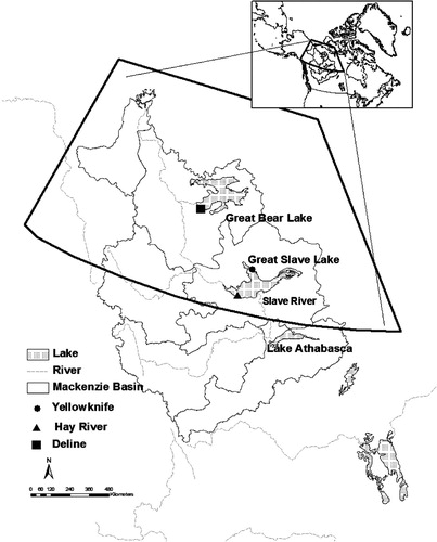
Table 1. Physical characteristics of GSL and GBL

Location	Latitude (°N)	Longitude (°W)	Z ML (m)	Z ROI (m)	Z Max (m)	Z Mean (m)	V (km^3)	A (km^2)
GSL					614	41	1580	27,000
Yellowknife station (Back Bay site)	62.46	114.44	10	10
Hay River station (Hay River site)	60.84	115.78	10	10
Main Basin (Main basin, GSL site)	61.50	114.6	40	80
GBL					446	72	2240	31,000
Deline station (GBL site)	65.21	123.44	40	60

Z _ML is the effective mixed layer depth.

Z _ROI is the actual lake depth at each site (region of interest, ROI).

Z _Max is the maximum depth.

Z _Mean is the average depth.

V is the lake volume.

A is the lake area.

Z _ML is used in CLIMo simulations (see explanation in Section 3.3).

3. Data and methods

3.1. Moderate Resolution Imaging Spectroradiometer

NASA MODIS land surface temperature data products are available as a series of seven products (5-min, daily, 8-d and monthly temporal resolutions at 1, 6 and 5.6 km spatial resolutions). The sequence begins as a swath (scene) at a nominal pixel spatial resolution of 1 km at nadir and nominal swath coverage of 2030 or 2040 lines (along track, about 5 min of MODIS scans) by 1354 pixels per line. Each product in the sequence is built from the previous products (Wan, 2007). The MODIS Terra and Aqua (Level 2, 1 km resolution, Version 5) daytime and night-time land surface temperature and emissivity products (MOD/MYD11_L2) derived from the thermal-infrared channels 31 and 32 were acquired through the NASA Land Processes Distributed Active Archive Center (LP DAAC) for the period 2002–2010. The products provide per-pixel temperature and emissivity values in a sequence of swath-based to grid-based (1 km gridded data set) global products and are produced daily at 5-min increments (the sensor acquires images in each 5 min).

The images were processed by averaging Terra, Aqua, day and night LST Level 2 products. The new algorithm is developed because there are no combined Terra and Aqua daily averaged products currently available. In this algorithm, first, the section of the file intersecting the region of interest is read, and then the latitude/longitude coordinates and time values are calculated for each pixel. The domain is split into approximately square tiles, which are re-projected to the Equal-Area Scalable Earth Grid (EASE-GRID) projection. The EASE-GRID projection consists of a set of three equal-area projections and developed at the National Snow and Ice Data Center (NSIDC) for the distribution of snow and ice products. It is intended to be a flexible tool for users of global-scale gridded data. The re-projection is carried out by first calculating the projection coordinates of each observation and then using linear interpolation to calculate a value for the centre of each EASE-GRID cell. Tiles of the selected regions of interest are then projected onto the target grid with the desired output resolution (1 km in this study) by averaging all pixels that fall into the target grid cell. The algorithm distinguishes daytime/night-time average data to be able to use each of them individually if needed. As there are two satellites (Terra and Aqua) operating a MODIS sensor, when combined it offers the possibility of four observations per day (two days and two nights). To produce daily LST products (day/night equal weight average), at least one daytime and one night-time observation is considered to keep the balance. For the entire domain, two sets of data are produced, one containing the average of all observations during the day and the other containing the observation during the night. Then, the intermediate sum of all MODIS Terra/Aqua day/night observations for each pixel is calculated. These values are averaged together to produce the final surface temperature average with equal weighting between day and night values.

These data, along with the day and night averages and the number of observations that went into producing each average, are output to a GEOTIFF file. The average (mean) daily values of pixels (one pixel from each region of interest) were extracted from the GEOTIFF files over the lake sites of Table 1 [Back Bay (GSL), Hay River (GSL), Main Basin (GSL) and Deline (GBL)] for comparison with the model simulations.

3.2. Canadian Ice Database

Lake ice thickness measurements and freeze-up/break-up dates from Back Bay (near Yellowknife, GSL) for the periods 1961–1996 were extracted from Canadian Ice Database (CID) (Lenormand et al., 2002) to evaluate the model results. For the period 1996–2002, no observations were taken (neither ice thickness nor freeze-up/break-up dates); however, they were resumed for 2002–2008. Ice thickness is measured approximately once a week, starting after freeze-up when the ice is safe to walk on, and continues until break-up when the ice becomes unsafe. Freeze-up and break-up dates, as defined herein, correspond to the earliest date on which the lake is completely covered by ice and the earliest date on which water is completely free of floating ice, as determined from an onshore observer (a person).

3.3. Canadian Lake Ice Model

CLIMo (Duguay et al., 2003) has been developed to simulate ice phenology, thickness and ice composition on lakes of various depths. This 1-D thermodynamic ice model has been tested extensively to simulate ice-growth processes on shallow lakes in Arctic/subArctic and high-boreal forest environments as well as on GSL (e.g. Duguay et al., 2003; Ménard et al., 2002; Morris et al., 2005; Brown and Duguay, 2011a Brown and Duguay, 2011b). For shallow lakes in the Churchill region, Manitoba, ice-on dates were simulated with 2 d accuracy in comparison with in situ observations (variation of mean absolute error), and break-up (ice-off) dates were simulated with 1–8 d accuracy depending on the on-ice snow depth scenario used in the simulations (Duguay et al., 2003). Ménard et al. (2002) also studied ice phenology using CLIMo on GSL for the period 1960–1991. Freeze-up and break-up dates were compared with in situ observations and those derived from the passive microwave satellite imagery. Results showed a good agreement between observed and simulated ice thickness and freeze-up/break-up dates for this period, particularly for Back Bay (4 and 6 d overestimation for break-up and freeze-up, respectively) and Hay River (4 and 5 d overestimation for break-up and freeze-up, respectively). It was further demonstrated that CLIMo is capable of reproducing well the seasonal and inter-annual evolution of ice thickness and on-ice snow depth, as well as the inter-annual variations in freeze-up and break-up dates (Ménard et al., 2002; Duguay et al., 2003; Jeffries et al., 2005; Brown and Duguay, 2011a Brown and Duguay, 2011b).

CLIMo performs surface energy budget calculations to obtain net flux at the ice, snow or open water surface, solving the 1-D heat conduction problem using an implicit finite difference scheme with the ice/snow slab discretised into an arbitrary number of thickness layers. The surface energy budget is expressed as:1

where F _o (Wm^–2) is the net downward heat flux absorbed at the surface, F _lw (Wm^–2) is the downwelling long-wave radiative energy flux, ɛ is the surface emissivity (ɛ is already being taken into consideration to F _lw since F _lw is a function of air temperature and atmospheric emissivity), σ is the Stefan–Boltzmann constant (5.67×10^–8 Wm^–2 K^–4), T (K) is the temperature, t (s) is the time, α is the surface albedo, I _o is the fraction of short-wave radiation flux that penetrates the surface (a fixed value dependent on snow depth), F _sw (Wm^–2) is the downwelling short-wave radiative energy flux, F _lat (Wm^–2) and F _sens (Wm^–2) are the latent heat flux and sensible heat flux, respectively. CLIMo uses the Shine (1984) and Maykut and Church (1973) parameterisation schemes to calculate short-wave and long-wave radiation, respectively. Shine (1984) improved the scheme of Zillman (1972) by adjusting its coefficients to better represent arctic winter conditions. Ice thickness growth is sensitive to the timing and amount of snow accumulation; therefore, snow cover plays an essential role in controlling the ice phenology of lakes (Duguay et al., 2003). CLIMo calculates ice and snow thickness from mass and density and computes the conductivity and heat capacity of the snow layer using the thermal conductivity of snow and a heat capacity parameterisation scheme, including the parameterisation of water vapour diffusion. Up to 99 layers can be specified in simulations to give a detailed temperature profile of the ice and snow (four ice layers and one snow layer were used in this study). CLIMo uses a surface albedo parameterisation, which takes into account the surface type (open water and snow/ice), surface temperature and ice thickness. The difference between the conductive flux and the net surface flux is used to calculate melting at the upper surface, with the intention that all snow is melted first and the remaining heat is used to melt the ice.

CLIMo includes a fixed-depth water mixed layer in a lake in order to represent a water surface temperature and ice annual cycle. When ice is present, the mixed layer is fixed at the freezing point; and when ice is absent, the mixed layer temperature is computed from the surface energy budget and hence represents a measure of the heat storage in the lake, namely:2

where T _mix is the mixed layer temperature, d _mix is the effective mixed layer depth and C _pw is the specific heat capacity of water (Duguay et al., 2003).

The daily averaged forcing data were obtained from the Meteorological Service of Canada weather station nearest to the sites. The forcing data used to simulate LST in GSL Main Basin are from the Yellowknife weather station, as there were no closer stations in this area of the lake. Data include daily 2-m air temperature, wind speed, relative humidity, cloud cover and snow depth. CLIMo uses snow depth measurements from the weather station closest to the lake as an input (forcing) and then calculates snow depth over the lake ice surface using different snow accumulation scenarios (Ménard et al., 2002; Duguay et al., 2003). These scenarios account for wind redistribution of snow on the open ice surface (0, 25, 50, 75 and 100% on the ice surface of the amount measured at the station onshore). In this study, a 50% snow cover scenario was used. Snow ice is also created by the model if there is a sufficient amount of snow to depress the ice surface below the water level. The added mass of the water-filled snow pores (slush) is added to the ice thickness as snow ice (Brown and Duguay, 2011b). Mixing depths of 10 m (Back Bay, Hay River) and 40 m (Main Basin-GSL, Deline-GBL) were selected based on the results from a previous investigation by Ménard et al. (2002) (see Table 1).

3.4. Freshwater Lake model

The FLake parameterisation scheme (Mironov, 2008; Mironov et al., 2010) is a computationally efficient FLake model, which is based on a two-layer water temperature profile, mixed layer at the surface and the thermocline extending from the bottom of the mixed layer to the bottom of the lake. The model is able to predict the surface temperature in lakes of various depths on the time scales from a few hours to a year. The structure of the stratified thermocline layer is described using the concept of self-similarity (assumed shape) of the temperature-depth curve. The same concept is used to describe the temperature structure of the thermally active upper layer of bottom sediments and of the ice and snow cover. The two-layer representation of the vertical temperature profile is:3

where θ _s (t) is the temperature of the upper mixed layer of depth h (t), κ _b is the temperature at the water-bottom sediment interface (z = D). Φ _θ (ξ)  ≡  [θ _s (t) – (z, t)]/[θ _s (t) – θ _b (t)] is a dimensionless function of dimensionless depth ξ≡[z – h (t)]/[D – h (t)] that satisfies the boundary conditions Φ _θ (0)  =  0 and Φ _θ (1)=1. The parameterised heat budget of the mixed layer when z is between 0 and h is:4

where ρ _w is the water density, C _w is the specific heat of water and Q _s and I _s are the value of the vertical turbulent heat flux and the heat flux due to solar radiation, respectively. Q _h and I _h are the heat fluxes at the bottom of the mixed layer (Mironov, 2008).

The main external parameter for the FLake model is the lake depth. For deep lakes, a virtual bottom depth of 40–60 m is typically used in simulations, instead of the real lake depth (Mironov, 2008) (using actual depth in deep lakes can lead to wrong results). FLake considers the snow cover over the lake ice surface, but this block was not tested and is not recommended to use. Therefore, the snow albedo is set equal to the ice albedo. The ice albedo is adapted to take into account the ageing of ice. FLake also takes into account wind-driven water mixing (which is an essential mechanism of the mixed layer growth) using a relaxation-type equation in stable situations. For convection regime, the entrainment equation is used.

FLake was forced by a time series of hourly atmospheric data. Forcing data were obtained from the weather stations nearest to the sites and consist of 2-m air temperature, wind speed and air humidity. The incoming short-wave and long-wave radiation fluxes were calculated from CLIMo and interpolated to hourly in FLake since no radiation fluxes are measured at the meteorological stations. In the absence of publicly available water transparency measurements for the studied lakes, the short-wave extinction coefficients were estimated based on knowledge of the general water transparency of the sites. As shown by Rouse and Duguay (2001), the semi-transparent nature of lake water allows incoming solar radiations to penetrate to considerable depth; therefore, lake water has a low surface albedo and absorbs incoming radiation. The authors reported that the maximum depths to which measurable solar radiation penetrated into lakes in the Yellowknife vicinity varied from 1.5 to 6.5 m. Thus, the short-wave absorption coefficient of water used in the simulations was 0.6 m^–1 for all GSL's study sites. Inflow and outflow water from Slave River and Hay River suspend sediments in the lake and are the main factors for the lower water transparency in GSL compared with GBL. The absorption coefficient in GBL site was set to 0.2 m^–1 since this lake is clearer as it does not receive any significant river inflow (Rouse and Duguay, 2001).

4. Results and discussion

LST values, ice thickness and freeze-up/break-up dates are compared between modelling results, MODIS (Terra/Aqua) observation data and in situ measurements from sites on GSL and GBL. The values of LST over the two large lakes are first plotted for the complete (full) years (January–December) (Figs. 2 and 3) and then separately for the open water season (June–October) (Fig. 4) and ice cover season (November–April) (Fig. 6). To assess the lake model results, three statistical indices were calculated: the mean bias error (MBE), the RMSE and the relative index of agreement (I _a). The MBE was calculated as model results minus MODIS (or in situ ice) observations. Hence, a positive (negative) bias indicates that modelled values are warmer (colder) than satellite measurements, have earlier (later) freeze-up/break-up dates, or thicker (thinner) ice. I _a is a ratio of the mean square error and the potential error, which is the largest value that the squared difference of each pair can attain (Wilmott, 1981). It is a descriptive measure applied to make cross-comparisons between models or models and observations, with possible values ranging from 0 (worst performance) to 1 (best possible performance) (Ménard et al., 2002). These indices have been shown to be robust statistical measures for validating model performance (e.g. Wilmott and Wicks, 1980; Hinzman et al., 1998).

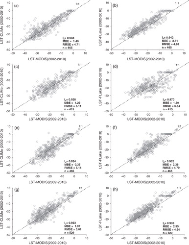
Fig. 2.  Comparison of modelled LSTs from CLIMo and FLake with MODIS-derived LSTs data during full year for 2002–2010: (a) Back Bay (Yellowknife station), (b) Hay River, (c) GSL (Main Basin) and (d) Deline-GBL.

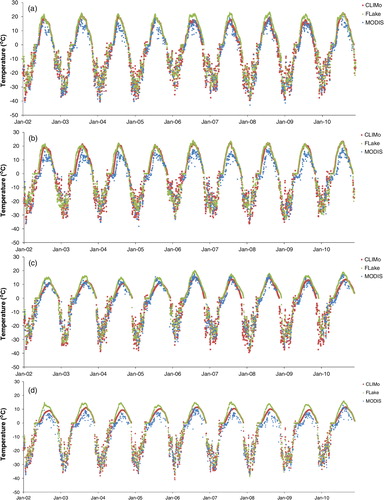
Fig. 3.  Comparison of modelled LSTs from CLIMo and FLake with MODIS-derived LSTs (°C) data during full year for 2002–2010: (a, b) Back Bay (Yellowknife station), (c, d) Hay River, (e, f) GSL (Main Basin) and (g, h) Deline-GBL.

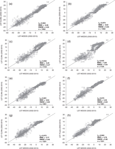
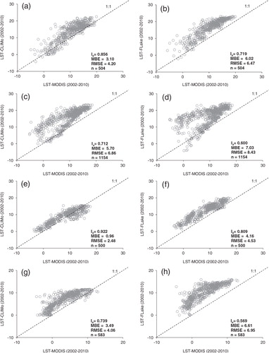
Fig. 4.  Comparison of modelled LSTs from CLIMo and FLake with MODIS-derived LSTs (°C) data during open water season for 2002–2010: (a, b) Back Bay (Yellowknife station), (c, d) Hay River, (e, f) GSL (Main Basin) and (g, h) Deline-GBL.

4.1. Lake surface temperature

Modelled LSTs from CLIMo and FLake are compared in Fig. 2 with MODIS-derived LST data for four different sites at GSL and GBL: Back Bay (near Yellowknife station), Hay River (near Hay River station), GSL (Main Basin) and Deline (near Deline station) over the full year (January–December) from 2002 to 2010. As Fig. 3 shows, both models show a good agreement compared to MODIS when data over the full year are considered (0.935  ≤  I _a  ≤  0.984; 0.94  ≤  MBE  ≤  4.83; 3.93  ≤  RMSE  ≤  7.64). A complete summary of the statistical indices is presented in Table 2. The performance of the two models is not the same on a seasonal basis. Hence, results were also examined separately for the open water and ice cover seasons. The periods of open water and ice cover seasons are chosen based on the break-up/freeze-up (ice off/ice on) dates from CID in situ observations for the period 1960–1996. Unfortunately, there were no in situ break-up/freeze-up date observations for the period 2002–2010 (only ice thickness). The observations showed that the average break-up date was 31 May and the average freeze-up date was 29 October (1960–1996). Therefore, in this study, open water period was selected from June to October and ice cover season was selected from November to April. The actual break-up/freeze-up dates change from year to year.

Table 2. Comparison of observed and simulated LST for Yellowknife (Back Bay), Hay River, GSL (Main Basin) and GBL (Deline) (2002–2010)

	Back Bay		Hay River		GSL(Main Basin)		GBL (Deline)
	CLIMo	FLake	CLIMo	FLake	CLIMo	FLake	CLIMo	FLake
Full year
I a	0.984	0.974	0.956	0.935	0.981	0.975	0.975	0.960
MBE	2.26	4.63	4.25	4.83	0.94	3.35	2.77	4.76
RMSE	4.30	5.64	6.27	7.64	3.93	4.63	4.45	5.82
Open water season
I a	0.860	0.719	0.712	0.600	0.922	0.809	0.739	0.569
MBE	3.10	6.02	5.70	7.03	0.96	4.16	3.49	6.61
RMSE	4.20	6.47	6.86	8.43	2.78	4.53	4.06	6.95
Ice cover season
I a	0.948	0.942	0.928	0.870	0.924	0.932	0.923	0.936
MBE	1.40	3.51	1.22	1.30	0.35	2.36	1.97	2.95
RMSE	4.71	4.98	5.11	6.54	5.14	4.79	5.01	4.64

4.1.1. Open water season.

Fig. 4 shows the comparison of open water season LSTs for the four selected study sites. The models show relatively warmer temperature than MODIS observations (0.96  ≤  MBE  ≤  7.03) for all four study sites. In the model simulations, the lake depths and the effective mixed layer depths for CLIMo were chosen as 10 m for Back Bay/Hay River and 40 m for Main Basin-GSL/Deline-GBL sites. The reason for the overestimation of temperature could be the forcing data used in models, which are taken from weather stations onshore not over the lake surface. During the spring, daytime air temperature over land could be several degrees warmer than over a colder lake, thus overestimating the simulated sensible heat flux.

For both models, the results for the Hay River site for LST show less agreement compared to Back Bay. Hay River is located at a lower latitude than the Back Bay site. The observed air temperature from the nearby weather station over this region of the lake is higher than the one at the Yellowknife station located in the Back Bay region (~2 °C warmer on average of 2002–2010). MODIS also shows on average 3.8 °C higher LST values for Hay River. Another reason for the warmer water temperature at the Hay River site is that the warmer water of the Slave River flows from the south into GSL from Lake Athabasca. The river water flows into the lake with a mean temperature of about 10–14 °C above the temperature of maximum density, which increases the temperature of this part of the lake (Schertzer et al., 2008). Howell et al. (2009) found that the break-up process of GSL starts first in this part of the lake due to discharge from the Slave River. Also, León et al. (2007) validated a 3-D lake hydrodynamics model, the Estuary and Lake COmputer Model (ELCOM), by using observed meteorological data and the output from the current Canadian RCM as forcing to compare the results with observed surface temperatures on GSL. The authors indicate that there are counter-clockwise dominant circulations patterns around the lake and a large central basin counter-clockwise gyre of the upper layer of this lake. This can at least partly explain the larger differences between simulated and observed LSTs of Hay River compared to the Back Bay site, as FLake and CLIMo are 1-D models and therefore do not simulate the lateral flow of warm water from a river that affects the Hay River site but not the Back Bay site. Although the river brings warmer water into the lake, MODIS observations still show lower temperatures than simulations. This can be explained by the time difference between the temperatures retrieved from MODIS in comparison with temperature measurements from weather stations (see Section 4.1.2). Also, it has been reported in other studies that MODIS generally tends to be slightly colder than in situ measurements of lake temperature (e.g. Crosman and Horel, 2009Crosman and Horel, 2009; a bias of −1.5 °C). In addition, Langer et al. (2010) presented surface temperature measurements from a field-deployed thermal infrared camera to evaluate MODIS Level 2 data at a Siberian polygonal tundra site. The authors found that some erroneous measurements can occur in the MODIS LST data during cloudy conditions (5–15 K colder temperatures from MODIS compared to those measured with the thermal camera) during the summer.

CLIMo-simulated LSTs are colder for all sites compared to those obtained with FLake. The lower surface temperature of CLIMo during summer may be explained by the fact that this model uses a constant (fixed) open water season mixed layer depth in each simulation, while the effect of the seasonally evolving mixed layer depth on the water surface temperature (reflected in MODIS LST measurements) is simulated with FLake (Fig. 5). The mixed layer depth is greater in late fall/early winter than in summer and depends on the water density and wind (Schertzer et al., 2008). In both the Back Bay and Hay River sites, the maximum mixing is occurring in late September. The increased temperature during the summer period leads to more stable density stratification and reduces the penetration of wind-driven mixing. The lake water has the highest density just before freeze-up and leads to a reduction in stability; therefore, the mixed layer increases in winter before an ice sheet is formed on the water body (Schertzer et al., 2008). The thermocline layer in GSL deepens almost monotonically from June–July to the period of complete mixing achieved in late September–October, as the temperature decreases due to the increase of surface heat losses to the atmosphere (Rouse et al., 2007). Since the mixed layer depth in CLIMo is fixed during the entire open water season, it will impact the seasonal evolution of open water LSTs calculated by this model compared to those either measured in situ or from MODIS.

Fig. 5.  Simulated mixed layer depth by FLake for 2002–2010: (a) Back Bay (Yellowknife station), (b) Hay River, (c) GSL (Main Basin) and (d) Deline-GBL.

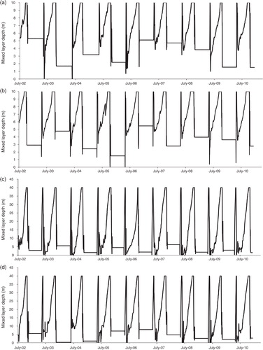
Given the above, LSTs from CLIMo tend to agree better with MODIS than those obtained with FLake for the two deepest lake sites (40 m). Complete mixing in the Main Basin-GSL and Deline-GBL occurs in late October–November, 1 month later than the shallower sites. As both models used are 1-D models, they do not take into account the numerous mixing mechanisms present in deep and large lakes, such as mechanical mixing, caused by 3-D water circulation, horizontal transfer of water by currents, etc. In CLIMo, the fixed mixing depth corresponds to strong vertical mixing in the first 40 m, thus suppressing the positive stratification in the initial open water period. On the other hand, in FLake, the thermal structure allows for stratification, with the mixed layer thickness much less than 40 m and it varies during the open water season. Thus, during the stratification period, the FLake LST is exceeding that of CLIMo. For the Main Basin-GSL, the behaviour of FLake LST is qualitatively closer to that of MODIS, although exaggerated, while CLIMo produces much longer warming and, consequently, longer autumn cooling than FLake, because of more heat accumulated in deeper mixed layer.

4.1.2. Ice cover season.

Simulated LST values from the models against MODIS-derived LSTs during the ice cover season are shown in Fig. 6. The figure shows CLIMo LSTs to be closer than those of FLake to the MODIS observations for all lake sites. MODIS shows relatively lower temperatures compared to the models, which can be partly explained by the time difference between the temperatures retrieved with MODIS and used to calculate daily averages in comparison with temperature measurements from weather stations that are used to force the models. Averaged hourly/daily air temperatures from the meteorological stations were calculated to force both models (FLake/CLIMo), but the crossing times for MODIS-Terra and MODIS-Aqua are at specific times at day and night, therefore not spread evenly over a full day (see Section 3.1). Averaged daily MODIS LSTs are generated when there are at least one day and one night observation under clear-sky conditions. It is possible that the calculated average comes from colder daytime or night-time acquisitions. Another reason for the colder MODIS LSTs can be explained by undetected clouds. The standard MODIS cloudmask product is used to create the MODIS LST Level 2 product. However, occasional undetected (cold) clouds exist in all cloudmask products (Wan, 2007).

Fig. 6.  Comparison of modelled LSTs from CLIMo and FLake with MODIS-derived LSTs (°C) data during ice cover season for 2002–2010: (a, b) Back Bay (Yellowknife station), (c, d) Hay River, (e, f) GSL (Main Basin) and (g, h) Deline-GBL.

Another important factor that has a direct impact on the models’ simulated LSTs is snow depth on the ice surface. As mentioned in Section 3.3, in FLake, the snow module has not yet been sufficiently tested and is not recommended for use, which is the primary reason for the weaker performance of this model (higher MBE values) during the winter season. In CLIMo, a 50% snow cover scenario was used in simulations during the ice cover season. This explains its better performance, as 50–70% of the snow measured at meteorological stations on land is generally a good average approximation of snow depth on open lake ice surfaces (Brown and Duguay, 2011a). Snow depths vary within the 1-km² pixels of MODIS and this is reflected in the satellite-retrieved LSTs, as conductive heat flow through lake ice is a strong function of snow depth and density (Jeffries and Morris, 2006). Thicker snow results in lower conductive heat transfer from the ice/water interface to the air/snow interface. Consequently, snow cover will influence the surface temperature over the lake during the ice cover season.

4.2. Ice thickness and phenology (Back Bay, GSL)

4.2.1. Ice thickness.

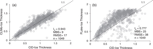
Figure 7 shows the simulated ice thickness from both models in comparison with in situ measurements for the period 1961–2008 at the Back Bay site. This is the only one of the four sites with a sufficiently long historical record for adequate comparison with model results, although there are data missing between 1996 and 2002. Results indicate a strong agreement between in situ measurements and CLIMo (I _a  =  0.943, MBE  =  9 cm, RMSE  =  17 cm), and a lower agreement with FLake (I _a  =  0.777, MBE  =  25 cm, RMSE  =  38 cm) (Fig. 8). As indicated earlier, FLake does not consider on-ice snow depth in this study. The accumulation of snow influences ice growth and thaw rates by adding an insulation layer. Previous results with CLIMo show that most of the variability in ice thickness and break-up dates is explained by on-ice snow (Duguay et al., 2003). In the FLake model, ice thickens more rapidly and also thaws faster compared to CLIMo and in situ measurements. The snow on the ice buffers the ice surface from the cold air above; consequently, the temperature at the bottom of snow is higher and less variable than the air temperature, and therefore ice grows at a slower rate than in the absence of snow (Jeffries and Morris, 2006). The above results indicate that the representation of snow on ice is an aspect that should be further developed and tested in FLake.

Fig. 7.  Comparison of observed (CID) and simulated (CLIMo and FLake) ice thickness (m) for Back Bay (1961–2008). Each dot in each year compares the in situ ice thickness values with the simulated one. There were about four in situ measurements available for each winter month.

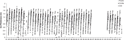
Fig. 8.  Comparison of observed (CID) and simulated ice thickness (m) for Back Bay: (a) CLIMo and (b) FLake (1961–2008).

4.2.2. Freeze-up/break-up

Both lake models reproduce freeze-up and break-up dates very well for Back Bay over the entire time series of observations (Figs. 9 and 10). As FLake does not consider the insulating effect of snow, it grows ice faster but also melts the ice faster. Compared with in situ observations, break-up dates simulated with FLake are therefore on average 6 d earlier and simulated with CLIMo are 3 d later (Table 3). In the presence of snow, the absorbed solar radiation is lower due to the higher albedo of snow compared to ice. In CLIMo, snow on ice is melted first before the ice, which can take several days (Duguay et al., 2006), while such snow is not represented in FLake. This is the most likely reason as to why FLake simulates average break-up dates earlier than CLIMo. For freeze-up dates, results between FLake (MBE  =  3 d, RMSE  =  7 d) and CLIMo (MBE  =  2 d, RMSE  =  7 d) are very similar when compared to observations (Table 3). An important factor on freeze-up dates is the lake depth (and depth of mixed layer). The greater the depth, the longer it takes for the ice cover to form. Ménard et al. (2002) showed that the best results with CLIMo are obtained with a mixed layer depth of 10 m for Back Bay.

Fig. 9.  Comparison of observed (CID) and simulated (CLIMo and FLake) (a) break-up and (b) freeze-up dates for Back Bay (1961–1996), Julian days.

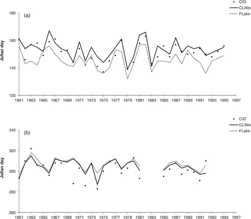
Fig. 10.  Comparison of observed (CID) and simulated (CLIMo and FLake) (a, b) break-up and (c, d) freeze-up dates for Back Bay (1961–1996), Julian days.

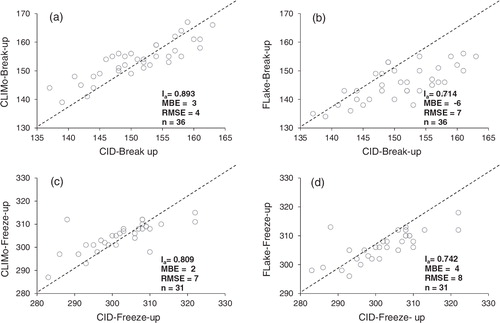
Table 3. Comparison of observed and simulated ice thickness and break-up/freeze-up dates for Yellowknife (Back Bay) site (1961–2008)

	CLIMo	FLake
Ice thickness
I a	0.943	0.777
MBE (cm)	9	25
RMSE (cm)	17	38
Break-up
I a	0.893	0.714
MBE (days)	3	–6
RMSE (days)	4	7
Freeze-up
I a	0.809	0.742
MBE (days)	2	3
RMSE (days)	7	7

5. Sensitivity experiment

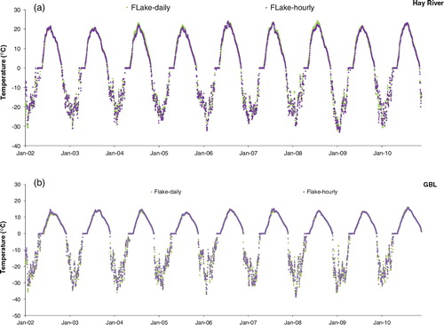
In the results described earlier, CLIMo was forced with daily averaged forcing data, as this is the current configuration and intended use of this model. FLake has also been used in a recent study to hindcast ice phenology using average daily forcing (Bernhardt et al., 2011). An additional experiment was carried out with the FLake model to determine the sensitivity of simulated LST and mixed layer depth when using daily averaged interpolated forcing compared to true hourly forcing. To our knowledge, this is the first time that FLake sensitivity to forcing data frequency has been tested to identify if, in the absence of true hourly forcing, linearly interpolated daily averaged inputs can be used instead, considering the same hourly time-step. The modelling experiment was conducted over the full study period (2002–2010) using a shallow lake site (Hay River) and a deep site (Deline-GBL). First, the model was forced using daily averaged data from Hay River and Deline weather stations and again using hourly data from the same stations. The model time-step of 1 h was used in both cases, but in the daily data-driven simulation the daily forcing values were linearly interpolated in order to obtain mock hourly forcing data. All other parameters such as lake depth, optical parameters and time-step were the same. As mentioned in Section 3.4, the incoming short-wave and long-wave radiation fluxes used in FLake were calculated from CLIMo. Therefore, the radiation fluxes were the same in both model runs and did not consider the daily cycle of short-wave radiation. Results show that on an annual basis the simulated LSTs do not differ much from each other (<0.3 °C on average during both the open water and ice cover seasons), hence the sensitivity to change from interpolated to true hourly data forcing is not high (Fig. 11).

Fig. 11.  Comparison of simulated LST by FLake using daily and hourly averaged forcing (a) Hay River-GSL and (b) Deline-GBL (2002–2010).

Table 4 shows the statistical differences of the two (hourly and daily) model runs compared to the MODIS satellite observations for the two lake sites and shows that the results do not differ greatly, with a slight improvement when using hourly forcing. Figure 12 compares the simulated mixed layer depth with hourly and daily forcing and shows that both lakes have the dimictic mixing regime with two seasonal overturning in late spring and late fall. In FLake, wind-driven and convection-driven water mixing is a highly non-linear process, which can affect the formation of mixing depth using daily or hourly forcing, but there is no wind-driven turbulence under ice in this model; therefore, the whole water column represents the thermocline layer (Martynov et al., 2010). The differences between hourly and daily forcing observed in this period of the year when lakes are covered with ice ranges from 0.32 to 6 m at Hay River-GSL and 0.25 to 6 m at Deline-GBL.

Fig. 12.  Comparison of simulated mixed layer depth by FLake using daily and hourly averaged forcing (a) Hay River-GSL and (b) Deline-GBL (2002–2010).

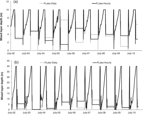
Table 4. Comparison of MODIS observed and simulated LST by FLake in Hay River, GSL and Deline, GBL (2002–2010) using daily forcing (FL_D) and hourly forcing (FL_A)

	Hay River		GBL (Deline)
	FL_D	FL_A	FL_D	FL_A
Full year
I a	0.929	0.935	0.962	0.960
MBE	5.12	4.83	4.58	4.76
RMSE	8.00	7.64	5.78	5.82
Open water season
I a	0.580	0.600	0.576	0.569
MBE	7.44	7.03	6.50	6.61
RMSE	8.87	8.43	6.84	6.95
Ice cover season
I a	0.861	0.870	0.937	0.936
MBE	1.38	1.30	2.67	2.95
RMSE	6.72	6.54	4.61	4.64

6. Summary and conclusion

MODIS-based LST (Level 2) day/night products from the Aqua and Terra satellites were obtained through NASA. A new average daily product was generated for each pixel using all available (day/night and Aqua/Terra) observations. Data from this product were used for comparison with LST simulation results obtained with two 1-D lake models (CLIMo and FLake) for GSL and GBL. In situ ice observations available for a site on GSL were utilised to evaluate the performance of both models. Simulations revealed that both models are capable of reproducing the seasonal and inter-annual evolution of the LST well, in addition to the inter-annual variations in ice thickness and freeze-up/break-up dates.

In experiments for GSL and GBL, both models demonstrated a good performance, especially when pooling data over the whole year simulation, when compared to MODIS and in situ measurements. The absence of snow in the FLake model had a large effect on ice growth and decay rates and thus, by extension, ice break-up dates. CLIMo simulated colder LSTs during the open water season compared to FLake due to the fact that the model uses a constant mixed layer depth while FLake simulates the seasonally evolving mixed layer depth. MODIS data showed generally colder temperatures compared to the models, which could be explained to some extent by undetected clouds (erroneous measurements during cloudy conditions) and the time differences of the MODIS LSTs (day and night observations) used to calculate clear-sky daily averages. Cloud contamination has been identified as a source of occasional (low temperature) errors in MODIS products (e.g. Langer et al., 2010). The best solution will be the improvement of the cloud mask, and this will be considered for future work. Moreover, the forcing data used for the models were from weather stations onshore. The air temperature over land could be some degrees warmer than over a colder lake, especially during the spring, which could cause an overestimation of simulated sensible heat flux resulting in a warmer simulated surface temperature.

Overall, the models showed a very good agreement with MODIS LSTs when calculating statistics over a full year, with some larger biases when years were divided into open water and ice cover seasons. LST data from MODIS or other thermal infrared satellite sensors such as AATSR are a promising data source for calibrating/evaluating lake models and should be explored for data assimilation experiments into NWP models. A more thorough evaluation of the accuracy of satellite-derived LSTs is also needed for northern lakes, as previous investigations have tended to focus on mid-latitude lakes during the open water season only.

Finally, results from the sensitivity experiment aimed at evaluating the impact of the true hourly forcing compared to interpolated hour forcing (from daily data) on FLake simulated LST and the mixed layer depth revealed that differences are very small. This suggests that on an annual basis, in the absence of hourly forcing data from weather stations, daily average forcing data are a viable alternative for simulations with FLake.

7. Acknowledgements

This research was supported by European Space Agency (ESA-ESRIN) Contract No. 4000101296/10/I-LG (Support to Science Element, North Hydrology Project) and a Discovery Grant from the Natural Sciences and Engineering Research Council of Canada (NSERC) to C. Duguay. We thank the anonymous reviewers for valuable comments and suggestions that helped improve the original manuscript.

References

- Bernhardt, J, Engelhardt, C, Kirillin, G and Matschullat, J. 2011. Lake ice phenology in Berlin-Brandenburg from 1947–2007: observations and model hindcasts. Clim. Change. 10.3402/tellusa.v64i0.17614.
- Brown, L. C and Duguay, C. R. 2010. The response and role of ice cover in lake-climate interactions. Prog. Phys. Geogr. 34(5), 671–704.
- Brown L. C. Duguay C. R. A comparison of simulated and measured lake ice thickness using a Shallow Water Ice Profiler. Hydrologic. Process. 2011a; 25(19): 2932–2941. doi: 10.1002/hyp.8087.
- Brown L. C. Duguay C. R. The fate of lake ice in the North American Arctic. Cryosphere Discuss. Cryosphere. 2011b; 5: 869–892. doi: 10.5194/tc-5-869.
- Coll C. Hook S. J. Galve J. M. Land surface temperature from the Advanced Along-Track Scanning Radiometer: validation over inland waters and vegetated surfaces. IEEE Trans. Geosci. Remote Sensing. 2009; 47: 350–360.
- Crosman E. T. Horel J. D. MODIS-derived surface temperature of the Great Salt Lake. Remote Sensing Environ. 2009; 113: 73–81.
- Duguay C. R. Flato G. M. Jeffries M. O. Ménard P. Morris K. Co-authors A. Ice covers variability on shallow lakes at high latitudes: model simulation and observations. Hydrologic. Process. 2003; 17: 3465–3483.
- Duguay C. R. Prowse T. D. Bonsal B. R. Brown R. D. Lacroix M. P. Co-authors A. Recent trends in Canadian lake ice cover. Hydrologic. Process. 2006; 20: 781–801.
- Eerola K. Rontu L. Kourzeneva E. Shcherbak E. A study on effects of lake temperature and ice cover in HIRLAM. Boreal Environ. Res. 2010; 15: 130–142.
- Hinzman L. D. Goering D. J. Kane D. L. A distributed thermal model for calculating soil temperature profiles and depth of thaw in permafrost regions. J. Geophys. Res. 1998; 103(D22): 28975–28991.
- Hostetler S. W. Bates G. T. Giorgi F. Interactive coupling of a lake thermal model with a regional climate model. Remote Sensing Environ. 1993; 98(D3): 5045–5052.
- Howell S. E. L. Brown L. C. Kang K. K. Duguay C. R. Monitoring lake ice phenology variability on Great Bear Lake and Great Slave Lake, Northwest Territories, Canada, from SeaWinds/QuikSCAT: 2000–2006. Hydrologic. Process. 2009; 113(4): 816–834.
- Jeffries M. O. Morris K. Instantaneous daytime conductive heat flow through snow on lake ice in Alaska. Annal. Glaciol. 2006; 20: 803–815.
- Jeffries M. O. Morris K. Duguay C. R. Lake ice growth and decay in central Alaska, USA: observations and computer simulations compared. Remote Sensing Environ. 2005; 40: 195–199.
- Langer M. Westermann S. Boike J. Spatial and temporal variations of summer surface temperatures of wet polygonal tundra in Siberia – implications for MODIS LST based permafrost monitoring. Hydrologic. Process. 2010; 114: 2059–2069.
- Lenormand F. Duguay C. R. Gauthier R. Development of a historical ice database for the study of climate change in Canada. Environ. Model. Softw. 2002; 16: 3709–3724.
- León L. F. Lam D. C. L. Schertzer W. M. Swayne D. A. Imberger J. Towards coupling a 3D hydrodynamic lake model with the Canadian regional climate model: simulation on Great Slave Lake. Tellus. 2007; 22: 787–796.
- Ljungemyr P. Gustafsson N. Omstedt A. Parameterization of lake thermodymanics in a high-resolution weather forcasting model. Boreal Environ. Res. 1996; 48A: 608–621.
- Martynov A. Sushama L. Laprise R. Simulation of temperate freezing lakes by one-dimensional lake models: performance assessment for interactive coupling with regional climate models. J. Appl. Meteorol. 2010; 15: 143–164.
- Maykut G. A. Church P. E. Radiation climate of Barrow, Alaska, 1962–66. Hydrologic. Process. 1973; 12: 620–628.
- Ménard P. Duguay C. R. Flato G. M. Rouse W. R. Simulation of ice phenology on Great Slave Lake, Northwest Territories, Canada. 2002; 16: 3691–3706.
- Mironov, D. V. 2008. Parameterization of Lakes in Numerical Weather Prediction. Description of a Lake Model. COSMO Technical Report, Deutscher Wetterdienst, Offenbach am Main, Germany, 11, 41.
- Mironov D. Heise E. Kourzeneva E. Ritter B. Schneider N. Co-authors A. Implementation of the lake parameterisation scheme FLake into the numerical weather prediction model, COSMO. Annal. Glaciol. 2010; 15: 218–230.
- Morris K. Jeffries M. Duguay C. R. Model simulation of the effects of climate variability and change on lake ice in central Alaska, USA. 2005; 40: 113–118.
- Rouse, W. R, Duguay, C. R. 2001. Modelling the energy and water balance of lakes in the cold regions of Canada. In: Proceedings of the 7th Annual Scientific Meeting of the Mackenzie GEWEX Study (MAGS). Hamilton, Ontario, Canada.
- Rouse, W. R., Binyamin, J., Blanken, P. D., Bussières, N., Duguay, C. R. and co-authors. 2007. The Influence of lakes on the regional heat and water balance of the central Mackenzie River Basin. In: Cold Region Atmospheric and Hydrologic Studies: The Mackenzie GEWEX Experience, (ed. Ming-ko Woo), Chap. 18, Vol. 1: Atmospheric Dynamics. Springer-Verlag, Berlin, Heidelberg, 309–325.
- Rouse W. R. Blanken P. D. Bussières N. Oswald C. J. Schertzer W. M. Co-authors A. An investigation of the thermal and energy balance regimes of Great Slave and Great Bear Lakes. Boreal Environ. Res. 2008; 9: 1318–1333.
- Samuelsson P. Kourzeneva E. Mironov D. The impact of lakes on the European climate as simulated by a regional climate model. 2010; 15: 113–129.
- Schertzer, W. M., Rouse, W. R., Blanken, P. D., Walker, A. E., Lam, D. C. L. and Leon, L. 2008. Interannual Variability of the Thermal Components and Balk Heat Exchange of Great Slave Lake. (ed. Ming-ko Woo), Chap. 11. In: Cold Region Atmospheric and Hydrologic Studies: The Mackenzie GEWEX Experience, Vol. 2: Hydrologic Processes. Springer-Verlag, Berlin, Heidelberg, 197–219.
- Schneider P. Hook S. J. Radocinski R. G. Corlett G. K. Hulley G. C. Co-authors A. Satellite observations indicate rapid warming trend for lakes in California and Nevada. Quart. J. R. Meteorol. Soc. 2009; 36: L22402. doi: 10.1029/2009GL040846.
- Shine K. P. Parameterization of the shortwave flux over high albedo surfaces as a function of cloud thickness and surface albedo. Phys. Geogr. 1984; 110: 747–764.
- Wilmott C. J. On the validation of models. Phys. Geogr. 1981; 2: 184–194.
- Wilmott C. J. Wicks D. E. An empirical method for the spatial interpolation of monthly precipitation within California. 1980; 1: 59–73.
- Wan, Z. 2007. Collection-5 MODIS Land Surface Temperature Products Users' Guide. ICESS, University of California, Santa Barbara.
- Zillman, J. W. 1972. A study of some aspects of the radiation and heat budgets of the southern hemisphere oceans. Meteorological Study, Vol. 26, Bureau of Meteorology, Department of the Interior, Canberra, Australia.