Implementations of a square-root ensemble analysis and a hybrid localisation into the POD-based ensemble 4DVar

ABSTRACT

The main purpose of this study is to propose a hybrid localisation technique for the proper orthogonal decomposition (POD)-based ensemble 4-D variational assimilation (PODEn4DVar) method with the aim of facilitating its implementation. This hybrid localisation scheme takes full advantages of both the implicit and explicit localisations and is relatively easy to be achieved by parallel programming. Besides, to strengthen its performance, we also incorporate a square root analysis scheme into the PODEn4DVar instead of its original one. The feasibility and effectiveness of the modified PODEn4DVar are demonstrated in a 2-D shallow-water equation model with simulated observations. It is found that the PODEn4DVar performs robust and is capable of outperforming the local ensemble transform Kalman filter (LETKF), its 4-D extension 4D-LETKF and another En4DVar method under both perfect- and imperfect-model scenarios.

• PODEn4Dvar
• square-root analysis
• hybrid spatial localisation
• En4Dvar

1. Introduction

The 4-D variational data assimilation (4DVar) method (e.g. Lewis and Derber, 1985; Courtier et al., 1994) provides a useful tool for data assimilation, owing to two attractive features: (1) the physical model can provide a temporal smoothness constraint and (2) it has the ability to simultaneously assimilate the observational data at multiple times in an assimilation window. Generally speaking, the emergence of the incremental method (Courtier et al., 1994) and adjoint technique (e.g. Lewis and Derber, 1985; Le Dimet and Talagrand, 1986; Courtier and Talagrand, 1987) brings about its successful applications in numerical operational weather prediction at many operational numerical weather forecast centres (e.g. Bormann and Thepaut, 2004; Park and Zou, 2004; Caya et al., 2005; Bauer et al., 2006; Rosmond and Xu, 2006; Gauthier et al., 2007). Increasingly, 4DVar shows promising results in data assimilation. However, 4DVar still faces numerous challenges in coding, maintaining and updating the adjoint model of the forecast model, and it requires the linearisation of the forecast model, especially when the forecast model is highly non-linear and the model physics contains parameterised discontinuities (Xu, 1996).

The ensemble Kalman filter (EnKF; e.g. Evensen, 1994, 2004; Houtekamer and Mitchell, 1998, 2001) is another advanced solution to data assimilation. EnKF becomes increasingly popular because of its simple conceptual formulation and relative ease of implementation. Compared with the traditional 4DVar, EnKF requires no derivation of a tangent linear operator or adjoint equations, and no integrations backward in time. Furthermore, the computational costs are affordable and comparable with other popular and sophisticated assimilation methods such as the 4DVar in the viewpoint of its easy parallel computing. By forecasting the statistical characteristics, EnKF provides flow-dependent error estimates of the background errors using the Monte Carlo method, but it lacks the temporal smoothness constraint as that in 4DVar, since it is naturally designed to incorporate sequential information only.

Large efforts have been devoted to seek to advance the state-of-the-science in data assimilation by coupling 4DVar with EnKF (e.g. Lorenc, 2003; Tian et al., 2008, 2011; Zhang et al., 2009; Cheng et al., 2010), aiming at exploiting the strengths of the two forms of data assimilation while simultaneously off-setting their respective weaknesses. A hybrid method, proper orthogonal decomposition (POD)-based ensemble 4-D variational assimilation (PODEn4DVar) method, was proposed by Tian et al. (2008, 2011) based on the Monte Carlo method and the POD technique. In the PODEn4DVar, the POD technique is applied to an ensemble of gridded 4-D observation perturbations (OPs) sampled from perturbed integrations of the forecast model at observational time levels to construct the orthogonal base vectors. Consequently, under the linear assumption between the model perturbations (MPs) and OPs, the perturbation ensemble in the model space is transformed in accordance with the POD transformation to the ensemble OP subspace. It guarantees the orthogonality (and thus independence) of the transformed OPs and their corresponding MPs. Furthermore, it can transform the original ensemble coordinate system into an optimal one in the L ² norm (Ly and Tran, 2001, 2002). As a result, the optimal MP and its corresponding OP can be expressed by the linear combinations of the transformed MPs and OPs, respectively, which substantially simplifies the implementation of 4DVar. Furthermore, the forecast ensemble, which provides flow-dependent error estimates of the background errors, can be updated continuously in an EnKF way (Evensen, 1994). More recently, based upon the PODEn4DVar, we have exploited a WRF-PODEn4DVar radar data assimilation system (manuscript in preparation). The preliminary results from real-data experiments suggest its potential performance for real atmospheric assimilation: it provides a promising new tool for data assimilation. Nevertheless, the experiments also indicate that the PODEn4DVar suffers from high computational costs due to its standard implicit localisation procedure. That seems to be particularly noticeable and should be specially addressed.

A main purpose of this article is to describe an implementation for the PODEn4DVar method that is both relatively easy to be achieved by parallel programming and computationally efficient. The emphasis here is to propose a hybrid localisation technique for the PODEn4DVar (but not limited to the PODEn4DVar method only), with the aim of facilitating its implementation. The localisation technique has been mainly developed in the EnKF community since it originally arises from ensemble-based assimilation methods. As a result, this article learns much from a number of EnKF studies (e.g. Hunt et al., 2007). The proposed hybrid localisation technique takes full advantages of both the implicit and explicit localisations, which allow the analysis to be done more efficiently as a parallel computation. Besides, inspired by the large number of existing ensemble analysis schemes, we also incorporate a square root ensemble analysis scheme into the PODEn4DVar instead of the original ensemble update implementation to mitigate its excessive confidence to the analysis mean.

For completeness, we first review the PODEn4DVar formulations and then incorporate a square-root ensemble analysis scheme into this approach in Section 2. The proposed hybrid localisation technique is described in Section 3. It is followed by observing system simulation experiments (OSSEs) for the evaluations of the PODEn4DVar in comparison to another ensemble-based 4DVar (En4DVar) method (Liu et al., 2008), the local ensemble transform Kalman filter (LETKF; Hunt et al., 2007) and its 4D case (4D-LETKF; Harlim and Hunt, 2007). Finally, some summary and concluding remarks are provided in Section 5.

2. The PODEn4DVar with a square-root ensemble analysis scheme

By minimising the following incremental form of the 4DVar cost function, one can obtain an optimal increment of the initial condition (IC), , at the initial time:1

where x′ = x–x _b is the perturbation of the background field x _b at t ₀:2 3 4 5 6

and7

Here, the superscript T stands for a transpose, b is the background value, index k denotes the observation time, S is the total number of observational time steps in the assimilation window, H _k is the observation operator, and matrices P _b and R _k are the background and observational error covariances, respectively.

The PODEn4DVar (Tian et al., 2011) starts from an ensemble of N OPs y′ : y′ ₁,y′ ₂,…,y′ _N , which are generated by using the observation operator H _k , the forecast model and the IC samples x′ : x′ ₁, x′ ₂,…,x′ _N . The POD of this OP matrix yields:8

and9

where Λ is a diagonal matrix of the singular values of y′ and V is an orthogonal matrix.

According to the assumption of linear relationship between the OPs and MPs [eq. (23) in Tian et al., 2011], the MP matrix is transformed as follows:10

Through the above POD transformations [eqs. (9) and (10)], the original ensemble coordinate system is transformed to an orthogonal and also an optimal one in the L ² norm (Ly and Tran, 2001, 2002) in the PODEn4DVar, which contributes a lot to its enhanced assimilation performance.

In consequence, the optimal solution and its corresponding optimal OP can be expressed by the linear combinations of the POD-transformed MPs and OPs, respectively, as follows:11

and12

Substituting eqs. (11) and (12) and the ensemble background covariance into eq. (1), the control variable becomes β instead of x′, and is expressed explicitly in the cost function:13

Through simple calculations (see Tian et al., 2011 for more details), the solution to the increment of analysis is simplified into the following form:14

Making , the final 4DVar analysis x _a can be calculated as follows:15

As illustrated in Tian et al. (2011), eq. (15) shares some similarity with the EnKF formulation in terms of the matrix acting as a proxy of the Kalman gain matrix as that in the EnKF analysis equation as long as the PODEn4DVar is degenerated to the 3-D case (PODEn3DVar). Under these circumstances, the relationship between the MPs and OPs is therefore simplified as y′=Hx′=H(x _b +x′)–H(x _b ), which implies:16

It is well known that in the EnKF:

where P ^f [i.e. P _b in eq. (1)] and P ^a are the background and analysis error covariances, respectively. Since , we have:17

by means of the similar transformations adopted in Hunt et al. (2007). On the other hand, P ^a=[1/(N–1)]X ^a (X ^a ) ^T , where X ^a is the analysis ensemble perturbation matrix, thus:18

The analysis ensemble perturbation matrix X ^a can be obtained by transforming the POD-transformed MPs P _x through a transform matrix . This type of ensemble analysis is known as an ensemble square root scheme.

The coupling strategy between the PODEn4DVar and its 3-D case proposed in Tian et al. (2011) is further improved in this study:

Firstly, the forecast model is initialised using the background fields x _b at t ₀ and then integrated throughout the assimilation window to obtain the 4-D background fields .

Secondly, the forecast ensembles X _b,k are obtained by the model integration from the initial ensemble X _b,0 sequentially over the same assimilation window. Thus, we can constitute the 4-D ensemble MPs:

and the 4-D ensemble OPs:

and then adopt the PODEn4DVar to produce the 4-D balanced analysis mean

Finally, the 3-D analysis ensemble perturbations at the kth time step are derived from the PODEn3DVar ensemble update process by utilising the 3-D ensemble MPs:

and their corresponding OPs:

Consequently, the forecast analysis ensembles X _a,k are achieved through for the next assimilation cycle.

In this way, the PODEn4DVar is used to update the ensemble mean by a 4DVar technique over each assimilation window, while the PODEn3DVar is used to update the ensemble perturbations in a 3DVar fashion (and solved by a square-root technique) for each observation time step included in the whole assimilation window.

It should be noted that the formulations of the PODEn4DVar are very similar with those of the 4D-LETKF (see Hunt et al., 2007 for more details). Again, it confirms the inherent relationship between 4DVar and EnKF that has been indicated by Hunt et al. (2007): EnKF is an equivalent procedure to accomplish the 3DVar with flow-dependent background covariances under the normal distribution assumption. Nevertheless, the PODEn4DVar mainly differs from the 4D-LETKF significantly in the following aspect: the use of the POD technique in PODEn4DVar transforms the original ensemble coordinate system into an optimal one in the L ² norm (Ly and Tran, 2001, 2002), which finally leads to its enhanced assimilation precision.

3. A hybrid localisation for the PODEn4DVar

An important issue in the ensemble-based method is sampling errors, and a practical way to address this issue is through a localisation (or inflation) technique, which could ameliorate the contaminations resulting from inadequate sampling or the spurious long-range correlations (Houtekamer and Mitchell, 2001). As demonstrated by Hunt et al. (2007), localisation is generally done either explicitly, considering only the observations from a region surrounding the location of the analysis (e.g. Houtekamer and Mitchell, 1998; Keppenne, 2000; Anderson, 2001; Ott et al., 2004), or implicitly by multiplying with a distance-dependent function that decays to zero beyond a certain distance, such that observations do not affect the model state beyond that distance (e.g. Houtekamer and Mitchell, 2001; Hamill et al., 2001; Whitaker and Hamill, 2002). In Tian et al. (2011), the PODEn4DVar adopted the implicit approach: the Schur product is applied to the matrix to filter out the remote correlation between the observation locations and model grids more continuously, and the final analysis is calculated using the formula:19

where the Schur product of two matrices having the same dimension is denoted by A=B∘C and consists of the element-wise product such that a _i,j =b _i,j ·c _i,j . For providing the formula of the filtering matrix, ρ, suppose K _x,i (i=1,…,L _x , where L _x is the length of vector x′) and K _y,j (j=1,…,L _y , L _y is the length of vector y′) are the model states and the observational variables, respectively. Making the horizontal and vertical distances between the spatial locations of K _x,i and K _y,j as d _h,i,j and d _v,i,j , respectively, then the elements of the matrix ρ can be calculated according to:20

where the filtering function C ₀ is defined as (Gaspari and Cohn, 1999):21

and d _h,0 and d _v,0 are the horizontal and vertical covariance localisation Schur radii, respectively. To accomplish this implicit localisation in eq. (19), one should first compute the matrix , which is high-computationally expensive and not easily achieved by parallel programming.

To alleviate this problem, we introduce a hybrid localisation approach as follows.

Equation (15) can be rewritten as:22

where . It implies each element x _a,i (i=1,…,L _x ) of x _a can be obtained through:23

where P _x,i is the ith row of P _x and x _b,i is the ith element of x _b . According to the filtering function [eqs. (19–20)], we can find that only the observations, which are located in the destined region (also see Fig. 1):24

Fig. 1.  Schematic diagram of the filtering matrix ρ.

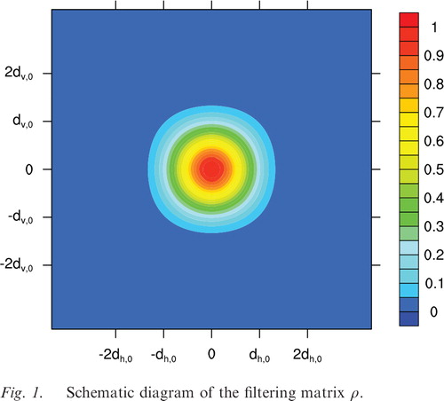
(x _a,i,h and x _a,i,v are the horizontal and vertical coordinates of x _a,i , respectively), contribute to the final grid analysis x _a,i . As a result of this, only those observation grids in the N×L _y matrix remain and constitute the N×L _y,g {L _y,g is the number of observation located in the region [eq. (24)]} local observation matrix , which accordingly leads to the simplification of eq. (23):25

We further implement the implicit localisation to eq. (25):26

which finally completes the formulations of the hybrid localisation for the PODEn4DVar. ρ _i is the filtering matrix for the model grid of x _b,i and its surrounding observation locations. Careful comparisons between eqs. (19) and (22–26) indicate that the two localisation schemes (i.e. the implicit localisation and the hybrid one proposed in this study) are actually equivalent: eqs. (23–26) jointly achieve the same function as the standard implicit localisation [eq. (19)]. The dimension of the local observation matrix in eqs. (25) and (26) is substantially lower than its counterpart of the original one in eq. (19), by which a lot of computational resources are thus released. In addition, the implementation of the local analysis is apt to be coded in parallelisation.

4. Evaluations within a shallow-water equation model

4.1. Shallow-water equation model

In this section, the PODEn4DVar with the hybrid localisation is evaluated by OSSEs with a 2-D shallow-water equation model (Qiu et al., 2007). The 2-D shallow-water equations are formulated in the f-plane by:27a 27b 27c

Here, f=7.272×10⁻⁵s⁻¹ is the Coriolis parameter; H=3000 m is the basic-state depth; h _s is the terrain height and is defined as:28

where h ₀=250 m for the true model or h ₀=0 m for the imperfect model, L _x =L _y =13 200 km are the lengths of two sides of the model domain, respectively, and the grid spacing is d=Δx=Δy=300 km. The model domain is a square with 45 × 45 grid points and its periodic boundary conditions at x=0 and L _x as well as y =0 and L _y are stipulated. The spatial derivatives are discretised by the second-order central finite difference scheme. The local time derivatives are discretised by using the two-step backward difference scheme of Matsuno (1966) to ensure the computation stability and restrain the effect of computational damping. The time step is Δt=360 s (=6 min). The model state vector is composed by the height h and the horizontal velocity components u and v at the grid points.

The “true” state is produced by integrating the “true” model (h ₀=250 m) with the following ICs at the very beginning of the integration (60 h before the starting time of the first data assimilation cycle):29a 29b

The model-produced “true” fields at t=0 are therefore achieved after 60 h integrations to the starting time of the first assimilation cycle. The “observations” are generated every 3 h by adding random noises to the above model-produced “true” fields at sparsely selected grids spaced every 3d=900 km in the x- and y-directions.

4.2. Experimental setup

In all the following OSSEs, the imperfect background state is produced by integrating the imperfect model (with h ₀=0 m) from t=−60 h [with the geostrophically balanced condition provided by eq. (29)]. Therefore, this background state is significantly different from the “true” state (not shown). Particularly, the spatially averaged root mean square (RMS) errors (calculated as differences between the model predicted background state and the “true” state) are 23.4 m, 1.53 and 2.58 m s⁻¹ for the h-, u- and v-fields, respectively.

The performance of the modified PODEn4DVar is examined in comparison to another En4DVar method (Liu et al., 2008), the LETKF (Hunt et al., 2007) and its 4-D case (4D-LETKF; Harlim and Hunt, 2007). Nevertheless, we will no longer involve the traditional 4DVar in the following experiments since its comparison with the previous version of PODEn4DVar (with no coupling strategy) has been discussed in Tian et al. (2008): Presumably, mainly a static background error covariance adopted in the standard 4DVar leads to its inferior performance. As aforesaid and also evaluated by Tian et al. (2011), the coupling strategy is really conducive to the improvement of assimilation performance. In consideration of this, we also implemented the proposed coupling strategy into both the En4DVar and the 4D-LETKF methods in our experiments. Thus, the two methods used here can be regarded as the modified versions of their original approaches. For the four assimilation methods, the ‘weight’ covariance inflation technique proposed by Zhang et al. (2004) is used to ‘relax’ or ‘weight’ the prior and update ensembles (the relaxation coefficient is set to α=0.9). In all the OSSEs, the time length of the data assimilation window is set to T=12 h. There are five observational levels in each assimilation window and the observational time interval is Δτ=3 h. Simulated observations are available in both the height and wind fields on a coarse grid and spaced every 3d=900 km in the x- and y-directions. The observation errors are uncorrelated for different variables and different points in space and time. The observation error standard deviations are 8 m for h and 0.9 m s⁻¹ for u and v. In addition, other standard parameter setups (also for the four assimilation methods) are the ensemble size N=100 and the covariance localisation Schur radius d _h,0=d _v,0=9.

4.3. Experimental results

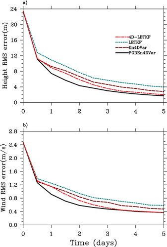
Figure 2 compares the performance of the PODEn4DVar with the En4DVar method, the LETKF and its 4-D case (4D-LETKF) under the perfect-model assumption (h ₀=250 m for the truth, forecast and assimilation runs). It shows that all the four methods behave considerably satisfactory in terms of overall low RMS errors, which is apparently attributed to the perfect-model assumption. The PODEn4DVar is the best performer among the four assimilation methods. It performs slightly better during the first assimilation window (0–12 h) and, after that, significantly better than the other three methods up to the end of the whole assimilation process. In the first assimilation window, the En4DVar shows almost identical performance with the 4D-LETKF because of their nearly same formulations except for the small differences in the ensemble analysis schemes: the En4DVar uses the most primitive ensemble analysis scheme while the 4D-LETKF updates its ensemble by means of a transform matrix in a square-root filter way (Hunt et al., 2007; Harlim and Hunt, 2007). Following this, under the perfect-model scenario, the superiority of the square-root analysis scheme in the 4D-LETKF beyond the primitive one adopted by the En4DVar appears more noticeable, which leads to the 4D-LETKF's lower RMS errors for both the height and wind fields than those of the En4DVar (Fig. 2a–b). In addition, the assimilation results also indicate that both the En4DVar and the 4D-LETKF perform substantially better than the LETKF. Intuitively, such phenomena are not difficult to be explained since the two former methods possess the basic advantages of 4DVar that the LETKF does not have. That is, they have the ability to simultaneously assimilate multiple-time observational data, and the physical model provides a temporal smoothness constraint. Moreover, their background error covairances are flow dependent and updated continuously since we have already upgraded the two methods by the coupling strategy that is originally adopted by the PODEn4DVar.

Fig. 2.  Spatially averaged (a) height RMS error and (b) wind RMS error for the four data assimilation methods [the PODEn4DVar (solid line), En4DVar (long-dashed line), LETKF (short-dashed line) and 4D-LETKF (dash-dot line)] without model error (h ₀=250 m), respectively.

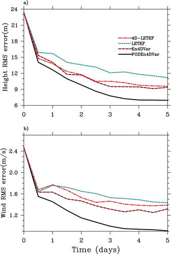
Another group of experiments with a severe model error is also conducted using a different maximum terrain height (h ₀=0 m) from that used in the truth simulation (h ₀=250 m). The truth run is used for verification and for generating observations. The experiment configurations are exactly the same as those for the perfect-model case. Figure 3 compares the performance of the four approaches with the imperfect forecast model (h ₀=0 m). Notably, in the presence of model error, the advantage of the PODEn4DVar over the other three methods becomes quite obvious, especially from the beginning of the second assimilation cycle to the end of the whole assimilation process. The same conclusion can be also obtained through the comparisons of their spatially mean RMS errors over the last assimilation cycle: the RMS errors for the PODEn4DVar are smallest for both the height and wind fields, respectively (only 6.94 m for the height and 0.90 m s⁻¹ for the wind). Since we have upgraded the 4D-LETKF approach by incorporating the coupling strategy, the only difference between the 4D-LETKF and our approach is whether the original ensemble coordinate system is optimised through the POD transformation or not. The results demonstrate that the POD-transformations adopted in the PODEn4DVar leads to its superior performance compared with the 4D-LETKF, especially under the imperfect-model assumption. The RMS errors produced by the PODEn4DVar and the 4D-LETKF methods averaged over the last assimilation cycle are increased from 6.94 to 9.57 m for the height and from 0.90 to 1.39 m s⁻¹ for the wind. Surprisingly, under the imperfect scenario, the En4DVar generally outperforms the 4D-LETKF a little, even though it uses the most primitive ensemble analysis scheme. Averaged over the last assimilation cycle, the RMS errors produced by the En4DVar and the 4D-LETKF methods are increased from 9.37 to 9.57 m for the height and from 1.32 to 1.39 m s⁻¹ for the wind.

Fig. 3.  Spatially averaged (a) height RMS error and (b) wind RMS error for the four data assimilation methods [the PODEn4DVar (solid line), En4DVar (long-dashed line), LETKF (short-dashed line) and 4D-LETKF (dash-dot line)] for the imperfect model (h ₀=0 m).

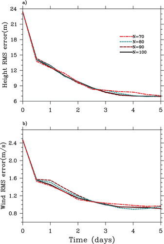
To discuss the impacts of the ensemble size on the PODEn4DVar assimilation results, four groups of experiments for the imperfect model (h ₀=0 m) using the PODEn4DVar method are conducted with the ensemble number N=90, 80, 70 and 60, respectively. Figure 4 shows that there are small differences among the four groups of the assimilation RMS errors with the ensemble number N=100, 90, 80 and 70, respectively. However, if the ensemble size is decreased to N=60, no convergence results are obtained (not shown). These experiments indicate that the PODEn4DVar can perform considerably robust as long as the ensemble size is not too small.

Fig. 4.  Spatially averaged (a) height RMS error and (b) wind RMS error for the PODEn4DVar for the imperfect model (h ₀=0 m) with the ensemble number N=100, 90, 80 and 70, respectively.

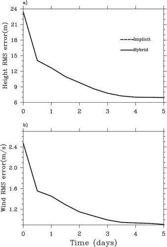
As has been noted previously, the purpose of this study is to alleviate the PODEn4DVar computational costs that are partially resulted from its localisation process and to code it by parallel programming easily without sacrificing any assimilation precision. To verify their equivalency of the implicit localisation and our hybrid one (actually the implicit one), we also compared the PODEn4DVar performances with the hybrid localisation scheme (referred to as “Hybrid”) and the implicit one (referred to as “Implicit”). Figure 5 demonstrates that the PODEn4DVar with the two localisation schemes (“Hybrid” and “Implicit”) can produce exactly the same assimilation results. Furthermore, for the two groups of experiments (both in serial programming), the ratio of the computational costs for the two schemes (“Hybrid” and “Implicit”) is about 0.93:1. Of course, this conclusion is not absolute and case-dependent because the scale of data assimilation varies greatly within different numerical models.

Fig. 5.  Spatially averaged (a) height RMS error and (b) wind RMS error for the PODEn4DVar with the hybrid localisation scheme (referred to as “Hybrid”) and the implicit one (referred to as “Implicit”) for the imperfect model (h ₀=0 m).

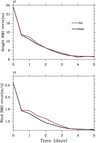
Finally, to investigate the choice of the original ensemble update method and the square root ensemble approach, we also designed another group of experiments using the PODEn4DVar with the original ensemble method (referred to as “Ori”) and the square root ensemble one (referred to as “New”) with the imperfect-model scenario, respectively. Figure 6 shows that the PODEn4DVar with the original ensemble update approach performs slightly worse than the square root ensemble case. Presumably, the original analysis update scheme tends to give more confidence to the analysis mean, which results in the narrower ensemble spreads and thus its inferior robustness.

Fig. 6.  Spatially averaged (a) height RMS error and (b) wind RMS error for the PODEn4DVar with the square root ensemble method (referred to as “New”) and the original one (referred to as “Ori”) for the imperfect model (h ₀=0 m).

5. Summary and concluding remarks

In this paper, the PODEn4DVar method proposed by Tian et al. (2008, 2011) is first upgraded by exploiting a square-root ensemble analysis scheme instead of its original one. This analysis scheme adjusts the model ensemble perturbations gradually by the PODEn3DVar (the 3D case of the PODEn4DVar) in the assimilation window through the proposed coupling strategy, which finally leads to its robust performance. Furthermore, a hybrid localisation approach is proposed with a view to alleviate the huge computational costs mainly resulting from its (PODEn4DVar) spatial localisation procedure. This methodology utilises ideas from both the implicit and the explicit localisation techniques. Particularly, this hybrid localisation can allow the analysis to be done more efficiently as a parallel computation. As far as the formulations are concerned, the modified PODEn4DVar is somewhat similar to the 4D-LETKF (Hunt et al., 2007; Harlim and Hunt, 2007). Nevertheless, two important characters (i.e. the POD-transformations to the MPs and OPs and the coupling strategy adopted in the PODEn4DVar) differentiate the PODEn4DVar from the 4D-LETKF and also another ensemble 4DVar method proposed by Liu et al. (2008), distinctly.

The robustness and potential merits of the modified PODEn4DVar are demonstrated by two sets of OSSEs performed with a 2-D shallow-water model. For comparisons, the En4Var, LETKF and 4D-LETKF are also adopted to conduct the same OSSEs under the same conditions. The main results are summarised as follows:

The method is robust even when the forecast model contains a significant bias error, and this is evaluated by the persistent convergence of the assimilation when the perfect model is replaced by the imperfect model.

The basic advantages of 4DVar imbedded in the three 4-D assimilation methods (PODEn4DVar, En4DVar and 4D-LETKF) lead to their superior performance compared to the LETKF.

The POD transformations conducted in the PODEn4DVar can transform its original ensemble coordinate system into an optimal one in the L ² norm (Ly and Tran, 2001, 2002), which makes the PODEn4DVar approach the best performer among the four assimilation methods involved in the OSSEs, especially when the forecast model is imperfect.

The hybrid localisation scheme proposed in this study is equivalent to the standard implicit one except for its easy parallel programming and lower computational costs.

The results obtained in this paper are encouraging. Furthermore, as explained in the introduction, we have exploited a WRF-PODEn4DVar radar data assimilation system based upon the proposed PODEn4DVar approach. On the basis of the hybrid localisation scheme proposed in this paper, parallel coding of the WRF-PODEn4DVar radar data assimilation system is ongoing.

6. Acknowledgements

This work was supported by the Knowledge Innovation Program of the Chinese Academy of Sciences (Grant No. KZCX2-EW-QN207), the National Natural Science Foundation of China (Grant No. 41075076) and the National Basic Research Program (Grant Nos. 2010CB428403 and 2009CB421407). Two anonymous reviewers are thanked for helpful comments and suggestions that improved both the presentation and the algorithms.

References

- Anderson J. L. An ensemble adjustment Kalman filter for data assimilation. Mon. Weather Rev. 2001; 129: 2884–2903.
- Bauer, P, Lopez, P, Benedetti, A, Salmond, D, Saarinen, S and co-authors. 2006. Implementation of 1D+4D-Var assimilation of precipitation affected microwave radiances at ECMWF II: 4D-Var. Q. J. R. Meteorol. Soc. 132, 2307–2332.
- Bormann N. Thepaut J. N. Impact of MODIS polar winds in ECMWF's 4DVAR data assimilation system. Mon. Weather Rev. 2004; 132: 929–940.
- Caya A. Sun J. Snyder C. A comparison between the 4DVAR and the ensemble Kalman filter techniques for radar data assimilation. Mon. Weather Rev. 2005; 133: 3081–3094.
- Cheng H. Jardak M. Alexe M. Sandu A. A hybrid approach to estimating error covariances in variational data assimilation. Tellus. 2010; 62A: 288–297.
- Courtier P. Talagrand O. Variational assimilation of meteorological observations with the adjoint vorticity equation II: numerical results. Q. J. R. Meteorol. Soc. 1987; 113: 1329–1347.
- Courtier P. Thepaut J. N. Hollingsworth A. A strategy for operational implementation of 4DVar using an incremental approach. Q. J. R. Meteorol. Soc. 1994; 120: 1367–1387.
- Evensen G. Sequential data assimilation with a nonlinear quasigeostrophic model using Monte Carlo methods to forecast error statistics. J. Geophys. Res. 1994; 99(C5): 10143–10162.
- Evensen, G. 2004. Sampling strategies and square root analysis schemes for the EnKF. Ocean Dyn. 54, 539–560. 10.3402/tellusa.v64i0.18375.
- Gaspari G. Cohn S. E. Construction of correlation functions in two and three dimensions. Q. J. R. Meteorol. Soc. 1999; 125: 723–757.
- Gauthier P. Tanguay M. Laroche S. Pellerin S. Morneau J. Extension of 3DVAR to 4DVAR: implementation of 4DVAR at the Meteorological Service of Canada. Mon. Weather Rev. 2007; 135(6): 2339–2354.
- Hamill T. M. Whitaker J. S. Snyder C. Distance-dependent filtering of background error covariance estimates in an ensemble Kalman filter. Mon. Weather Rev. 2001; 129: 2776–2790.
- Harlim J. Hunt B. R. Four-dimensional local ensemble transform Kalman filter: numerical experiments with a global circulation model. Tellus. 2007; 59A: 731–748.
- Houtekamer P. L. Mitchell H. L. Data assimilation using an ensemble Kalman filter technique. Mon. Weather Rev. 1998; 126: 796–811.
- Houtekamer P. L. Mitchell H. L. A sequential ensemble Kalman filter for atmospheric data assimilation. Mon. Weather Rev. 2001; 129: 123–137.
- Hunt B. R. Kostelich E. J. Ott E. Szunyogh I. Efficient data assimilation spatiotemporal chaos: a local ensemble transform Kalman filter. Physica D. 2007; 230: 112–126.
- Keppenne C. L. Data assimilation into a primitive-equation model with a parallel ensemble Kalman filter. Mon. Weather Rev. 2000; 128: 1971–1981.
- Le Dimet F. X. Talagrand O. Variational algorithms for analysis and assimilation of meteorological observations: theoretical aspects. Tellus. 1986; 38A: 97–110.
- Lewis J. M. Derber J. C. The use of the adjoint equation to solve a variational adjustment problem with advective constraints. Tellus. 1985; 37A: 309–322.
- Liu C. Xiao Q. Wang B. An ensemble-based four-dimensional variational data assimilation scheme. Part I: technique formulation and preliminary test. Mon. Weather Rev. 2008; 136: 3363–3373.
- Ly H. V. Tran H. T. Modeling and control of physical processes using proper orthogonal decomposition. Math. Comput. Model. 2001; 33: 223–236.
- Ly H. V. Tran H. T. Proper orthogonal decomposition for flow calculations and optimal control in a horizontal CVD reactor. Q. Appl. Math. 2002; 60: 631–656.
- Lorenc A. The potential of the ensemble Kalman filter for NWP: a comparison with 4DVar. Q. J. R. Meteorol. Soc. 2003; 129: 3183–3203.
- Matsuno T. Numerical integration of the primitive equations by a simulated backward difference method. J. Meteorol. Soc. Jpn. 1966; 44: 76–84.
- Ott, E, Hunt, B. R, Szunyogh, I, Zimin, A. V, Kostelich, E. J and co-authors. 2004. A local ensemble Kalman filter for atmospheric data assimilation. Tellus. 56A, 415–428.
- Park K. Zou X. Toward developing an objective 4DVAR BDA scheme for hurricane initialization based on TPC observed parameters. Mon. Weather Rev. 2004; 132(8): 2054–2069.
- Qiu, C, Shao, A, Xu, Q and Wei, L. 2007. Fitting model fields to observations by using singular value decomposition: an ensemble-based 4DVar approach. J. Geophys. Res. 112, D11105. 10.3402/tellusa.v64i0.18375.
- Rosmond T. Xu L. Development of NAVDAS-AR: nonlinear formulation and outer loop tests. Tellus A. 2006; 58(1): 45–58.
- Tian, X, Xie, Z and Dai, A. 2008. An ensemble-based explicit four-dimensional variational assimilation method. J. Geophys. Res. 113, D21124. 10.3402/tellusa.v64i0.18375.
- Tian X. Xie Z. Sun Q. A POD-based ensemble four-dimensional variational assimilation method. Tellus. 2011; 63A: 805–816.
- Whitaker J. S. Hamill T. M. Ensemble data assimilation without perturbed observations. Mon. Weather Rev. 2002; 130: 1913–1924.
- Xu Q. Generalized adjoint for physical processes with parameterized discontinuities. Part I: basis issues and heuristic examples. J. Atmos. Sci. 1996; 53(8): 1123–1142.
- Zhang F. Snyder C. Sun J. Tests of an ensemble Kalman filter for convective-scale data assimilation: impact of initial estimate and observations. Mon. Weather Rev. 2004; 132: 1238–1253.
- Zhang, F. Q, Zhang, M and Hansen, J. A. 2009. Coupling ensemble Kalman filter with four dimensional variational data assimilation. Adv. Atmos. Sci. 26(1), 1–8. 10.3402/tellusa.v64i0.18375.