Impacts of cloud flare-ups on hurricane intensity resulting from departures from balance laws

ABSTRACT

Cloud flare-ups along the inner eye wall of a hurricane lead to enhancement of cloud scale divergence, which in turn leads to a large local enhancement of the departure from balance laws and can lead to local supergradient winds. This scenario is tested using the results from a mesoscale microphysical model at horizontal resolution of 1.33 km for the simulation of hurricane Katrina. Rainwater mixing ratio tags growing cloud elements. The departure from balance laws includes terms such as the local, horizontal and vertical advections of divergence, divergence square and a term invoking the gradient of vertical velocity. It is noted that these terms collectively contribute to a substantial local enhancement of the departure from balance laws. Departures from balance laws are related to the radial gradient wind imbalances in a storm-centred coordinate. In this study, several examples, from the hurricane Katrina simulations, that display this scenario of rapid intensification are illustrated. Organisation of convection in the azimuthal direction seems important for the hurricane scale; cloud flare-ups away from such regions of azimuthal organisation fail to contribute to this scenario for the overall intensification of the hurricane.

• hurricane intensity
• hurricane modelling
• clouds within hurricanes
• flights in hurricanes
• hurricane dynamics
• inner core hurricane

1. Introduction

A number of external and inner core processes seem to impact the hurricane intensity. The outer angular momentum of inflowing air parcels in a hurricane, as it is depleted by various torques, such as the cloud torques, relate to the hurricane intensity (Krishnamurti et al., 2005). Numerous inner core processes also seem to have a large impact on the hurricane intensity. These include cloud microphysical processes (Braun and Tao, 2000; McFarquhar and Black, 2004; Rogers et al., 2007). Pattnaik and Krishnamurti (2007a, 2007b) noted sensitivities of hurricane intensity from processes such as the melting of snow, ice and graupel and the evaporation of falling hydrometeors. The eye wall replacement is yet another phenomenon that contributes to hurricane intensity changes. The importance of cloud flare-ups along the eye wall (Hennon, 2006) was noted as a factor that was often associated with the rapid intensification of a hurricane.

The importance of the oceanic heat content has been stressed by several authors (Jaimes and Shay, 2009). Their studies on the general region of the loop current of the Gulf of Mexico, from the analysis of Airborne Expendable Bathythermograph (AXBT) data sets, showed many mesoscale subsurface thermal features in the upper Gulf of Mexico waters. They noted impacts on intensity changes for hurricanes Katrina and Rita, of the year 2005, from the large heat content of the upper oceans.

Intensity changes have also been attributed to the intrusions of dry air and dust into the inner core of hurricanes. There are also several studies, Montgomery and Kallenbach (1997), Montgomery and Enagonio (1998), on the dynamics of the inner core where the passage of vortex Rossby waves and their interactions with the inner core convection have been related to intensity changes. Diagnostic studies based on data assimilated fields on mesoscales for hurricanes were examined by Simon et al. (2010), and they noted that a number of dynamical parameters exhibit large changes during periods of rapid intensity changes in hurricanes. These parameters included the vertical differential of heating in the complete potential vorticity (PV) equation, where heating generates lower tropospheric PV in the inner core of hurricanes. That increase in PV results in an increase of vorticity since static/thermodynamic stability decreases in these regions and accounts for an increase of storm intensity. Other factors in this diagnostic study included the energy exchange function between the divergent kinetic energy to rotational kinetic energy, the transformation of shear vorticity to the curvature vorticity in the inner core and the advections of the earth and relative angular momentum into the inner core of hurricanes in a storm relative frame of reference.

The present study examines model output from a high-resolution hurricane simulation that was performed by Davis et al. (2008). This was a study on the modelling of the intense phase of hurricane Katrina of the year 2005 at a horizontal resolution of 1.33 km. These simulations were reasonable in capturing the intensity and track of this hurricane during its passage over the Gulf of Mexico. An interesting outcome of an examination of the model output was a scenario where often cloud bursts along the inner wall of the model hurricane were accompanied by a growth of lower tropospheric convergence, a growth of departure from balance laws and a growth of supergradient winds. We shall describe these aspects of the model dynamics in the context of the rapid intensity change of hurricane Katrina.

In a recent modelling study of a hurricane, Smith and Montgomery (2008) compared the full mesoscale model evolutions with those from a balanced model in the planetary boundary layer and noted that the departures from the balanced model were quite large in the complete model that included the physical processes in its parameterisations. Their study focused on the limitations of balance models for a hurricane. Our results are consistent with their findings; however, this study is different from theirs in relating cloud bursts to the growth of gradient wind departures (GWDs) and the supergradient winds in the context of the rapid intensification issue.

Several important studies, Nguyen et al. (2008) and Gopalakrishnan et al. (2011), provide relevant background for the findings here. Nguyen et al. (2008) showed the importance of vertical hot towers via the sequence of cyclonic rotation of the hot towers and their eventual aggregation, whereas Gopalakrishnan et al. (2011) provided a thermal plume theory for the rapid intensification. These studies did not directly examine the possible low-level convergence beneath their elements. It is certainly possible that the cloud flare-up issue is related to these findings. An integrated study of all these elements is needed.

2. Model simulation of hurricane Katrina

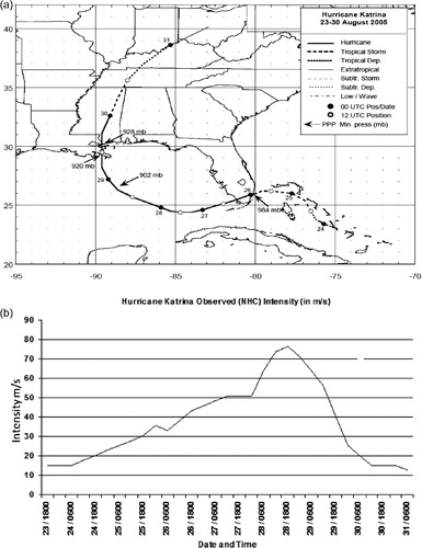
There have been several recent studies on hurricane Katrina that address predictive aspects of modelling (Bender et al., 2007; McTaggart-Cowan et al., 2007a, 2007b; Mainelli et al., 2008 and several others). Data sets from a recent study of Davis et al. (2008) that carried out experiments at a very high horizontal resolution for Katrina is utilised for this study. It is noted that their results for intensity, track and structure forecasts appeared reasonable when compared to the assimilated fields. In this section we shall describe a few aspects of this National Center for Atmospheric Research Weather Research and Forecasting/Advanced Research WRF (NCAR WRF/ARW) model and present some major results from this experiment for the forecasts of hurricane Katrina. The observational aspects of Katrina are well summarised in Knabb et al. (2005). The track and intensity of Katrina, provided by the National Hurricane Center, are presented in Fig. 1a,b. Katrina started moving northwestward along the western periphery of the ridge on 27 August 2005 and produced tropical-storm force winds and heavy rainfall over western Cuba. The eye wall sharpened into a well-defined ring by 0000 UTC 28 August, and in less than 12 hours Katrina became a Category 5 hurricane with winds reaching 145 knots (1 knot=0.5144 m/s) by 1200 UTC 28 August. In another 6 hours Katrina reached its peak intensity of 150 knots (1 knot=0.5144 m/s). The eye wall started eroding late on 28 August and Katrina weakened to a Category 3 hurricane with an intensity of 110 knots (1 knot=0.5144 m/s) when it made landfall near Buras, Louisiana. It finally made another landfall near Pearl River at the Louisiana/Mississippi border still as a Category 3 hurricane with 105 knots winds (1 knot=0.5144 m/s). This model carried an outer grid of 12 km horizontal resolution and movable inner grid domains of 4 km and 1.33 km. The Kain-Fritsch cumulus parameterisation (Kain and Fritsch, 1993; Kain, 2004) was used uniformly for the outer 12 km mesh; the inner high-resolution nests carried explicit clouds without any cumulus parameterisation. The model included a state-of-the-art cloud microphysics following Hong et al. (2004). For the planetary boundary layer, a first-order closure scheme was based on Noh et al. (2003). The surface drag follows the Charnock (1955) formula, where the water vapour fluxes at the surface were estimated following Carlson and Boland (1978) and the heat flux is based on the Skamarock et al. (2005) scheme. While most forecasts were started at 0000 UTC, some during landfall periods were initiated at 1200 UTC. Each of these Katrina forecasts with the WRF/ARW model utilised the initial states from the operational Geophysical Fluid Dynamics Laboratory (GFDL) forecasts that were available at the horizontal resolution of 1/6 degree latitude/longitude.

Fig. 1.  (a) Best track positions of Hurricane Katrina (Adapted from Knabb et al., 2005, Tropical Cyclone Report, Hurricane Katrina 20–30 August 2005). (b) Observed Intensity (NHC) for Hurricane Katrina in ms⁻¹.

2.1. Intensity prediction by the WRF/ARW model for hurricane Katrina

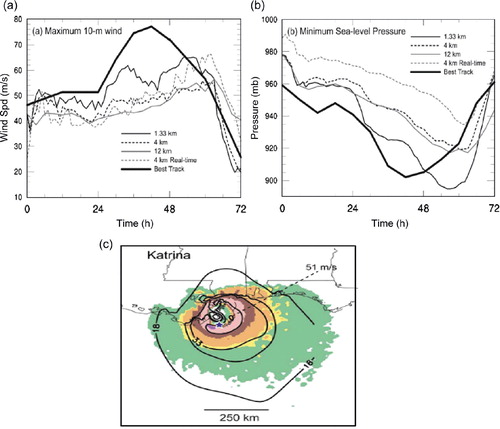
The results of 72-hour forecasts for the intensity of Hurricane Katrina are illustrated in Fig. 2a,b. These two illustrations, respectively, show the maximum 10-m winds and the minimum sea level pressure for the predicted hurricane. There are five sets of curves in these illustrations, which include forecasts made by the model at resolutions 1.33, 4 and 12 km for a real-time forecast effort at NCAR using the WRF/ARW, and the best estimates for validation provided by the National Hurricane Center. Although there was a phase shift by almost 12 hours in the best forecasts provided by the 1.33 resolution model, in general the highest resolution provided the best intensity forecasts. The maximum winds were experienced during the life cycle of Katrina on 28 August 2005 at 1800 UTC. The observed strongest winds and minimum sea level pressure were 76.5 m/s and 902 hPa, respectively. The corresponding numbers for the prediction at 1.33 km resolution were 67 ms⁻¹ and 897 hPa, respectively, when the model had peak intensity. Given this level of success from the mesoscale model we were motivated to carry out post-processing diagnostics of the model data that is described in Sections 3 and 4 of this article.

Fig. 2.  (a) Maximum 10-m wind and (b) minimum sea level pressure for forecasts of Katrina beginning 0000 UTC 27 August. Legend labels 1.33, 4 and 12 km refer to grid spacing of WRF ARW, version 2.1.2, using the Charnock drag relation. The forecast on a 12-km grid used the Kain–Fritsch parameterisation. The 4-km real time (grey dashed) refers to the forecast made in real time with an innermost nest of 4-km grid spacing. All retrospective forecasts were initialised with the GFDL initial condition. (c) The 10-m wind from WRF/AHW real-time forecasts (shaded) with contours of HWind analyses overlaid for hurricane Katrina. Predicted storm centre location at indicated valid times (below) is denoted by blue star in the figure. Wind fields from AHW forecasts have been shifted to observed locations to facilitate comparison. Model valid times is 1200 UTC 29 August (60-h forecast) (Adapted from Davis et al., 2008).

2.2. Prediction of 10 m winds

In Fig. 2c the 60 hour predicted winds, at 10 m, for Hurricane Katrina from the study of Davis et al. (2008) are shown. These predicted wind speeds are shown in colour (shaded), superimposed on top are the HWIND (contours) from hurricane Research Division (HRD). The HWIND is an in-house wind analysis product of HRD, which incorporates all the wind observations from a variety of observing platforms and develops an objective analysis of the distribution of winds in a hurricane (Powell and Houston, 1998; Powell et al., 1998). Basically the purpose of showing this superposition of wind strengths from the model and HWIND is to confirm that the model at the horizontal resolution of 1.33 km is able to describe a reasonable spread of the isotachs outwards from the centre of the hurricane. The model winds are at 1200 UTC on 29 August 2005, whereas the HWIND observations were centred at 1132 UTC on the same date. Overall we see a close match for the size and strengths of the predicted winds compared to these observed estimates.

Davis et al. (2008) also noted several other interesting features from the modelling. They found that the best wind fields were simulated at the inner core nest of 1.33 km, as compared to those at the 4 km and 12 km. They also displayed the model-based radar reflectivities for the 1.33 and 4 km inner nest and showed that the 1.33 km inner nested movable grid provided results that were close to those seen from reconnaissance aircraft radar for hurricane Katrina.

3. Implication of GWDs for hurricane intensity

The GWD as noted from a storm-centred local cylindrical coordinate is an important aspect of this study.

The full divergence equation can be written in the form (Fankhauser 1974):1

where V _θ is the tangential wind, V _r is the radial wind, D is the divergence, ω is the vertical velocity, FV _θ and FV _r denote the frictional forces per unit mass along the tangential and radial directions.

The underlined terms represent the balance equation (Haltiner and Williams, 1980). The other terms denote the rotational part non-linear balance (Krishnamurti, 1968) and is expressed by:2

It should be noted that the divergence equation for the non-linear balance is eq. (2), which is what is used to find the rotational part of the wind (i.e. the streamfunction here). However, the vorticity equation, scaled to the non-linear balance, retains parts of the twisting/tilting terms following Phillips (1963).

Next, a discussion of balance wind departures in local cylindrical storm-centred coordinates are presented. The complete radial equation of motion is expressed as:3

4

If GWD is equal to 0, then:4a

Equation (4a) represents the gradient wind equation (in storm-centred coordinate, along the radial direction).

where GWD denotes the gradient wind departure, that is:5

V _θ can be expressed by the relation:6

This includes the GWDs. This is a local value of the tangential wind from the complete radial wind equation in the presence of GWDs. Note that is generally<0 in the inner rain area (r<200 km, where r is positive outward), since the geopotential, z, increases outwards in a hurricane. The gradient wind, in this local storm-centred coordinate, is given by:7

For a hurricane in storm-centred coordinates the radial gradient wind equation is expressed by where , fV _θ and are all generally positive. The roots of this equation are:8

Note that the negative root of the radical is non-physical; hence there is only one positive root, that is for . This implies that applies for cyclonic motions. Note that there are no anomalous solutions of the radial gradient wind equation, that is there is only one normal solution. Thus, several possibilities exist because of the sign and magnitude of GWDs. If we have a non-physical solution. We are looking for different options for , which represents a physical solution. Since we can write the inequality in the form, .

The left-hand side is essentially positive definite, GWD<0 would always satisfy this condition. If GWD is positive and if the above inequality is satisfied we can still have a physical solution. A negative value of GWD contributes to a value of V _θ in eq. (5), which is supergradient; hence extreme negative values of GWD would go with large values of azimuthal motions, that is supergradient winds. A positive value of GWD can describe situations with subgradient winds.

Strong azimuthal motions, described by the complete radial equation of motion, are attributed to the (GWDs), which relate to large values of divergence. The non-linear balance and the radial gradient wind equation are equivalent since they both represent balanced conditions. It is easy to show that the rotational part of the gradient wind balance along the radial direction is equivalent to the radial part of the non-linear balance equation (see Appendix).

Departures from non-linear balance largely arise from horizontal and vertical advection of divergence and the divergence squared. If a flare-up of deep convection occurs near the eye wall of a hurricane, divergence (/convergence) increases, so do the departures from balance laws. Growth of negative departures leads to local supergradient winds. This follows from:9

GWD′ denotes all those terms of the complete divergence equation that are not in the non-linear balance equation (2). Likewise, GWD denotes all the terms of the complete radial wind equation that are not contained in the radial gradient wind equation (4a).

We have routinely mapped the field of GWD′ in the intensifying and decaying phases of hurricane intensity and noted that as divergence/convergence increases so do the GWDs. The GWD for the local cylindrical coordinate GWD is quite similar to GWD′. In principle, GWDs are computed from subtracting the gradient wind from the total wind. Our procedure, in the end, is exactly that. The analysis, based on the full non-linear balance equation and gradient wind equation, is presented here since it provides a better insight into this problem.

Both GWD′ and GWD denote balanced states of the atmosphere, one is the departure from the non-linear balance and the other is the departure from the radial gradient wind balance. To derive the latter from the former, one needs to take the rotational parts of the vector equation of motion and examine the radial (local cylindrical) resulting equation that yields the radial gradient wind equation (without any divergent components). That is the amount of equivalence one can demonstrate for these two balanced states. The neglected terms carry smaller magnitudes in the radial equation since the rotational dynamics is dominant. Those are, however, of interest because of systematic departures from the gradient wind balance during cloud flare-ups.

4. Example of cloud flare-up in the model output

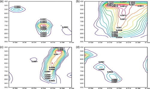
Hennon (2006) examined the relationship of cloud flare-ups and the intensity from data sets within hurricanes. Her study makes use of the rapid scan imagery from the GOES satellite and the aircraft reconnaissance-based winds (dropwindsonde and flight level). She examined as many as 344 cloud burst events during a three-year period and provided an exhaustive statistical analysis of these events with respect to hurricane size, geographical distributions of storms and frequencies of occurrence of rapid intensification. The flare-up of deep convection, along the inner eye wall of a hurricane determined, by using model-based fields of cloud water mixing ratio, the rain water mixing ratio, or the radar reflectivity estimated from the model predicted hydrometeors, is presented here. The typical life cycle of a deep convective cloud is of the order of a few hours. Figure 3 illustrates one such life cycle where the cloud grows, covering the deep troposphere in a matter of an hour, and decays in another hour. The cloud outline is provided by the 0.0001 kg kg⁻¹ isopleth. During the course of integration of hurricane Katrina, several such cloud growths along the inner eye wall of the hurricane were noted. Elsewhere in the outer radii some cloud growths that were seen in the model simulated radar reflectivity were also noted. We shall be addressing some of these in this article.

Fig. 3.  The life cycle of a deep convective cloud shown at different times (a) 1500 UTC 28 August 2005; (b) 1600 UTC 28 August 2005; (c) 1700 UTC 28 August 2005; (d) 1800 UTC 28 August 2005. The cloud outline is provided as the 0.0001 kg kg⁻¹ isopleth.

5. Examples of build-up of deep convection, divergence, departure from balance laws and supergradient winds

In Figs. 4, 5, 6 and 7, respectively, the hourly predicted histories of the vertically integrated liquid water mixing ratio (between surface and the 450 hPa level), the divergence at the 850 hPa level, the departure from the balance laws and the model-based total wind [which is also the solution of eq. (6), when applicable] are shown. These features can also be displayed by overlaying the four fields (geographically) on top of each other. These cover the hours 1500 UTC to 1800 UTC for 28 August 2005; these were 39 and 42 hours of forecasts. The scale below each illustration provides the range of values for each field, and the units are provided in the respective figure captions. At the horizontal resolution of 1.33 km these are robust fields in a developing hurricane. A strong relationship between the cloud water mixing ratios and the field of convergence is seen at the 850 hPa level. The fields of the departures from balance laws at the 850 hPa level also depict stronger values where the liquid water mixing ratios are large. They include the eye wall and the rain band regions of the model predicted hurricane Katrina when it was intensifying. The 10-m level (vertical level above the earth's surface) isotachs of the total wind from the model output in Fig. 7 show large hour-by-hour changes in the belt of the strongest winds. At those locations where GWD is negative, or small positive, and a root of eq. (6) is available, these isotachs also represent the solution based on eq. (5). Overall this is a robust isotach field during an intense phase of a hurricane, with the strongest winds in excess of 60 ms⁻¹.

Fig. 4.  The hourly time history of vertically integrated liquid water from surface to 450 hPa levels for (kg kg⁻¹) (a) 1500 UTC 28 August 2005; (b) 1600 UTC 28 August 2005; (c) 1700 UTC 28 August 2005; (d) 1800 UTC 28 August 2005.

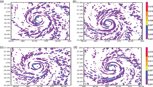
Fig. 5.  The typical hourly time history of divergence (s⁻¹) at the 850 hPa level. (a) 1500 UTC 28 August 2005; (b) 1600 UTC 28 August 2005; (c) 1700 UTC 28 August 2005; (d) 1800 UTC 28 August 2005.

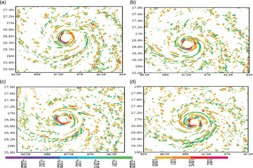
Fig. 6.  The typical hourly time history of non-balance (×10⁻⁵ s⁻²) at the 850 hPa level. (a) 1500 UTC 28 August 2005; (b) 1600 UTC 28 August 2005; (c) 1700 UTC 28 August 2005; (d) 1800 UTC 28 August 2005.

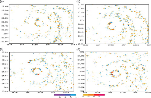
Fig. 7.  The typical hourly time history the intensity of hurricane (ms⁻¹). (a) 1500 UTC 28 August 2005; (b) 1600 UTC 28 August 2005; (c) 1700 UTC 28 August 2005; (d) 1800 UTC 28 August 2005.

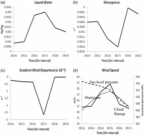
Figure 9 shows the hourly time evolution of parameters from Figs. 4, 5, 6 and 7 at a specific point where the model produced a sudden build-up of deep convection. These are based on hourly model output data sets. The location of these points is marked as A, B, C and D in Fig. 8 where the bursts of deep convection were noted. During these events we noted that the liquid water mixing ratio increases from roughly 0.001 kg kg⁻¹ to almost 0.006 kg kg⁻¹. The enhancement of lower tropospheric convergence at this location increased from roughly 5×10⁻⁴ to 4.5×10⁻³. The hourly data show these as rapidly increasing events. The departures from balance laws show a rapid increase from −0.5×10⁻⁵ to −2.5×10⁻⁵. During this event the observed wind increases from roughly 30 ms⁻¹ to 75 ms⁻¹. Figures 9, 10, 11 and 12 show such examples for cloud flare-up events. These effects of flare-ups to produce an intensification of the entire hurricane may take several hours since the flare-ups shown in Figs. 9, 10, 11 and 12 are local features that first occur at individual locations. A question of some interest is possible time lags among these parameters. We could not find a sufficient sample of cloud bursts to quantitatively say anything definitive about possible lags. These hourly data sets seem to suggest, from just four cases, that the bursts of deep convection precede the other parameters by roughly an hour. This could imply that the local increase of buoyancy, brought about by differential advection of temperature and/or moisture at different levels, could initiate this scenario resulting finally in a local growth of supergradient winds. To have a large part of a hurricane show rapid intensification may however require more than a single cloud burst. These four examples of Figs. 9–12 were all cloud elements that were located close to the inner eye wall of the predicted hurricane Katrina. These events occurred close to the time of rapid intensification of Katrina. The rapid intensification of Katrina to a Category 5 on the Saffir-Simpson scale storm occurred at around 1800 UTC on 28 August 2005.

Fig. 8.  Location of the points where deep convection was noted are indicated as letters A, B, C and D and a location outside the eye wall is marked with a letter N.

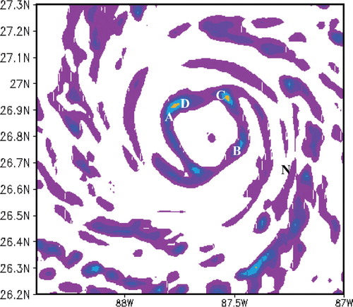
Fig. 9.  An example of hourly (along abscissa) changes, of the (a) cloud liquid water (kg kg⁻¹), (b) divergence s⁻¹, (c) gradient wind departures (×10⁻⁵ s⁻²) and the (d) wind speed (ms⁻¹) as solid line and sea level pressure marked as dashed line (hPa), along the ordinates, for the simulated hurricane Katrina. The azimuthal average wind is shown by short dashes and labelled as hurricane. These are results for a cloud flare up event indicated in Fig. 8 as A along the inner eye wall.

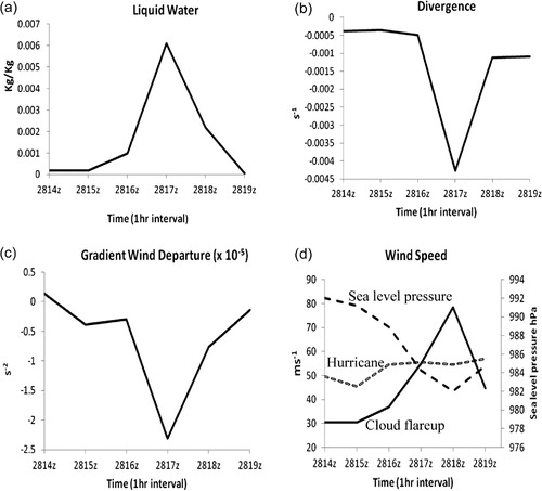
Fig. 10.  Same as Fig. 9, but for another selected cloud flare up event (B in Fig. 8).

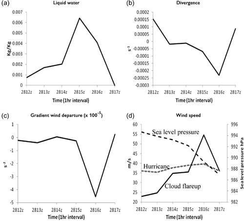
Fig. 11.  Same as Fig. 10, but for another selected cloud flare up event (C in Fig. 8).

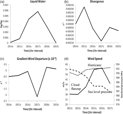
Fig. 12.  Same as Fig. 11, but for another selected cloud flare up event (D in Fig. 8).

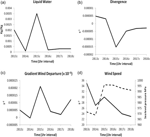
Figure 13 illustrates the results for a cloud burst event that occurred away from the inner eye wall at a radius of roughly 50 km from the model hurricane's centre. This is indicated with letter N in Fig. 8. The cloud burst was noted from the liquid water mixing ratio increasing from roughly 0.0001 kgkg⁻¹ to 0.0037 kgkg⁻¹ (Fig. 13a), over a two-hour period. The corresponding increase of convergence at the 850 hPa level is shown in Fig. 13b. In spite of the increase of convergence, this location carried largely a growth of positive values (Fig. 13c) for the departure from the gradient wind balance as the cloud burst occurred. The gradient wind equation that carries positive values for departures does not have a physical solution, and we cannot see a supergradient solution at this location. The model-based winds at this location are shown in Fig. 13d, which does not carry any perceptible growth of the wind related to the cloud burst. This shows that there are locations where we can see the scenario of cloud burst, growths of convergence, negative GWDs and generation of supergradient winds, and there are other locations where the GWDs carry an opposite sign, and at those locations no strengthening of winds is noted. We have examined nearly all the grid points of the model and noted these features.

Fig. 13.  An example of hourly (along abscissa) changes, (a) of the cloud liquid water (kg kg⁻¹), (b) divergence s⁻¹, (c) gradient wind departures (×10⁻⁵ s⁻²) and the (d) wind speed (ms⁻¹) as solid line and sea level pressure marked as dashed line (hPa) along the ordinates, for the simulated hurricane Katrina on 28 August 2005. This cloud element indicated as N in Fig. 8 is located well outside of the inner eye wall.

It is of interest to ask what signatures at sea level can be seen during the cloud flare-up events. For illustrating these features we have included the time history of the sea level pressure for the cloud burst events in Figs. 9d, 10d, 11d and 12d. The sea level pressure drops during the course of each such event. These features confirm that the cloud burst affects the sea level pressure and is a robust factor, as was also noted from the time history of the deep tropospheric θe (described later). The cloud burst is associated with the storm intensification as was noted in Figs. 9, 10, 11 and 12. The cloud burst is a robust tropospheric phenomenon, which leaves its signature in a number of parameters such as sea level pressure, and the deep vertical structures of θe and moisture. The sea level pressure starts to drop as a cloud burst begins and often keeps dropping as that cloud element grows. This is noted in all cases of cloud bursts that are presented here. The increase in wind speed and the dropping of pressure seem to go together. These are based on single grid points, where the cloud burst was tagged from the liquid water mixing ratio. Often the pressure continues to drop for roughly an hour after the maximum wind of the cloud burst was noted; this has to do with the overall size of the element that requires displaying several adjacent grid points. The entire field is not shown for convenience, but the important point is that a significant pressure drop is noted during the cloud burst. Such a feature was, however, not seen when a cloud grew well outside of the eye wall region (Fig. 13d). Here the pressure change with time has an entirely different signature with no relationship to the winds, which also did not display any intensification.

It is important to ask if the overall hurricane wind speed shows an intensification when the local wind speed strengths following a cloud burst. The azimuthally averaged wind is also plotted in panel (d) of Figs. 9, 10, 11, and 12 for the four cloud burst events. These are winds at the 10-m level. This azimuthal average wind is shown by short dashes and labelled as hurricane. In all instances of cloud burst an overall increase of the azimuthally averaged wind speed during the four events is noted. This suggests a contribution by the cloud flare-up events to the overall intensification of the model hurricane.

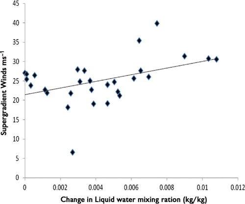
A scatter plot of points where the change in liquid water content is positive between two hours (1500 and 1600 UTC of 28 August 2005, when the hurricane was intensifying) with respect to supergradient winds is shown in Fig. 14. The abscissa in this diagram denotes the difference between the total wind from the model and the computed radial gradient wind that is a measure of the supergradient part of the total wind. The large supergradient winds carry amplitudes as much as 40 ms⁻¹. The computations of supergradient winds were done following eqs. (6) and (7). This scatter plot shows only those points where there was a simultaneous presence of large positive change of the liquid water content and of the supergradient winds. The scatter plot clearly suggests an increase of supergradient winds over regions where the liquid water content also showed a rapid increase. These computations were done to illustrate the relationship between cloud flare-ups and rapid intensification. While a single flare-up of a cloud along the inner eye wall may not be expected to cause the intensification of a hurricane, the simultaneous occurrences of several flare-ups could contribute to the generation of supergradient winds at several locations that can flow through advective process in a few matter of hours and contribute to intensification.

Fig. 14.  Scatter plot of points where the change in liquid water content (kg kg⁻¹) is positive between two hours 1500 UTC and 1600 UTC of 28 August 2005 when the hurricane was intensifying with respect to supergradient winds (ms⁻¹) at 1600 hours of 28 August 2005.

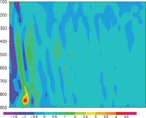
Figure 15 shows an azimuthally averaged radial height cross section of the GWDs. This illustration confirms the inherent nature of GWDs in the inner core of a hurricane. Hence dynamical studies of the imbalances are important for the hurricane intensity issue. The negative values of the GWDs abound in this azimuthal average, signify the presence of supergradient winds over such regions.

Fig. 15.  Azimuthally averaged radial height cross section of the gradient wind departures, in 10⁻⁵ s⁻² (pressure, in hPa, along ordinate and radial distance, in km, along the abscissa) for a cloud flare up event.

5.1. Evolution of temperature anomaly

The time history of the west to east cross section of the temperature anomaly (anomaly prepared with respect to the Jordan sounding for the hurricane season) is shown in Fig. 16 across one of the four cloud flare-up points. This flare-up point is located along the inner eye wall of the model predicted hurricane. A warm anomaly is clearly seen in all these sections with maximum amplitude of roughly 16°C, and the largest amplitude of the warming is located near the 250–300 hPa levels. This illustration confirms that the cloud flare-up plays a role in amplifying the warm core of the model hurricane. Collectively a number of such flare-ups (not shown here) seem very important for the intensification of the modelled hurricane Katrina.

Fig. 16.  Time history of the west to east cross section of the temperature anomaly (anomaly prepared with respect to the Jordan sounding for the hurricane season) for a cloud flare-up event: (a) 1430 UTC 28 August 2005; (b) 1530 UTC 28 August 2005; (c) 1630 UTC 28 August 2005; (d) 1730 UTC 28 August 2005.

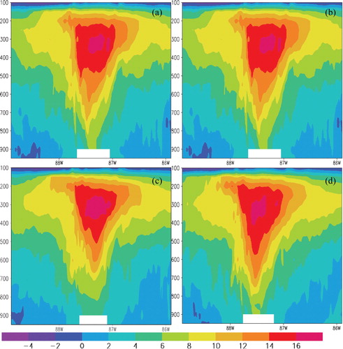
A related question is whether the azimuthally averaged cross section of the modelled hurricane shows a robust warm core, which is being strengthened during the occurrence of the cloud flare-ups. The time evolution of the azimuthally averaged cross section of the temperature anomaly covering the period of the cloud burst event is illustrated in Fig. 17. These sections show an expansion of the warm core radially with a robust thermal anomaly, near 16 °C, when the model hurricane Katrina was intensifying. One can thus relate the cloud flare-up process contributing to the intensification of the axisymmetric component of the hurricane.

Fig. 17.  Time history of the west to east cross section of the azimuthally averaged cross sections of temperature anomaly, in degree centigrade (pressure, in hPa, along ordinate and radial distance, in km, along the abscissa) for a cloud flare-up event: (a) 1430 UTC 28 August 2005; (b) 1530 UTC 28 August 2005; (c) 1630 UTC 28 August 2005; (d) 1730 UTC 28 August 2005.

5.2. Cloud burst carves out an eye like feature for the equivalent potential temperature

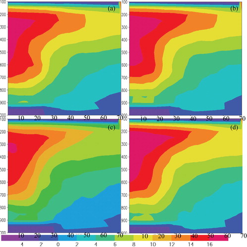
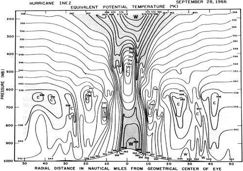
A time sequence of west to east vertical cross sections of the equivalent potential temperature θe, roughly one hour apart, across a cloud burst, are shown in Fig. 18. The well-known vertical cross section of θe for hurricane Inez, Hawkins and Imbembo (1976), is also shown in Fig. 19. The typical cross section shows a near constant θe profile along the vertical in the eye wall region and lobes of minimum θe on either side outside the eye wall that are located near the 600 hPa level. This is the region that is conditionally unstable, and the lower tropospheric inflowing air of the hurricane constantly provides that instability to the eye wall region where it is eroded by deep convective mixing. When a cloud burst occurs in such an unstable region, very soon that newly forming deep convection carves out an eye like feature, showing also the side lobes of the θe minimum. Here we show one example of a cloud burst, along the inner eye wall, that was illustrated earlier in Fig. 8. This sequence of illustrations of the θe cross sections of Fig. 18 clearly shows the cloud burst is attempting to reinforce by making a contribution that resembles Fig. 19. This suggests that robust cloud bursts reinforce the azimuthally organised convection towards strengthening the θe features of a hurricane eye region.

Fig. 18.  Time history of the west to east cross section of the equivalent potential temperature (units: degrees Kelvin) (pressure, in hPa, along ordinate and radial distance, in km, along the abscissa) for a cloud flare-up event: (a) 1430 UTC 28 August 2005; (b) 1530 UTC 28 August 2005; (c) 1630 UTC 28 August 2005; (d) 1730 UTC 28 August 2005.

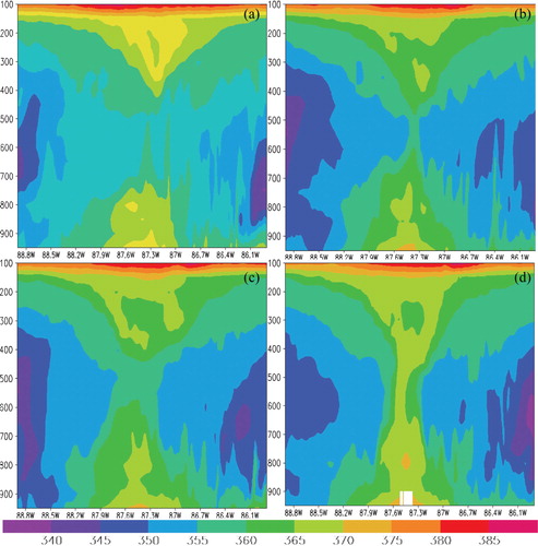
Fig. 19.  Vertical cross section of equivalent potential temperature for Hurricane Inez on 28 September 1966 (Hawkins and Imbembo, 1976).

5.3. Response of surface fluxes during cloud flare-ups

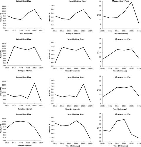
The fluxes of moisture, sensible heat and momentum all showed a response to the cloud flare-ups. In Fig. 20 we present the surface fluxes for each of the cloud flare-up events (previously presented in Fig. 8). Of interest here is the increase of surface fluxes during each of the flare-up events: 300–500 watts/m² enhancement of the latent heat fluxes 50–200 watts/m² enhancement of sensible heat fluxes and 2–6 Pa enhancement of momentum fluxes were seen during these cloud flare-up events. It was difficult to assess any systematic lags between the flare-up of the liquid water mixing ratios and the flare-ups of these surface fluxes; it appeared that at best those events were nearly simultaneous within a half-hour interval. The main message conveyed by these computations is that these flare-ups are deep tropospheric events involving surface fluxes and the entire thermodynamic structure of the equivalent potential temperature. A number of studies of Emanuel (1986, 1988, 1997) relate the maximum hurricane intensity and the hurricane intensification issues to surface latent heat fluxes and to the prevailing Sea Surface Temperatures (SST) anomalies. The cloud bursts can occur in consort with such processes at the lower boundary. That is a possibility worthy of further exploration. We have also seen buoyancy elements that are present near the cloud base level, with life times of the order of 12 hours that seem to be advected by the prevailing winds and precede the cloud flare-ups. Whether selectively some of these buoyancy elements are triggered by the surface physics has not been explored here.

Fig. 20.  An example of hourly (along abscissa) changes, of the latent heat flux (watts/m²), sensible heat flux (watts/m²), momentum flux (pa) as solid line, along the ordinates, for the simulated hurricane Katrina for the same locations shown in Figs. 9–12. These are results for a cloud flare up event along the inner eye wall.

6. Organisation of convection

The issue of organisation of convection along the azimuths of a model hurricane following our recent study, Krishnamurti et al. (2005), is addressed in this section. That method simply entails asking what the variances are for any variable at the different azimuthal wave numbers. This analysis is generally performed along the inner eye wall region of a hurricane. The azimuthal harmonic analysis is done for variables such as the tangential velocity, rain or cloud water mixing ratios, or the model hydrometeor's implied radar reflectivity. The results show that a mature hurricane is largely explained by azimuthal wave numbers 0, 1, 2 (85% of the total azimuthal variance). This simply means that single deep convective cloud elements that may erroneously seem to be contributors for azimuthal wave numbers 24 or 25 (based on their scales of a few kms) are in fact organised along with other cloud elements along the azimuth, and they end up directly contributing to the variance for the very low wave numbers 0, 1 and 2. Single cloud bursts often contribute to the increase of the hurricane scale azimuthal variance, where the hurricane scale is identified by low azimuthal wave numbers 1, 2 and 3. This implies an organisation of convection on the hurricane scale.

Some three to four deep mesoconvective systems distributed around the hurricane provides this large variance for these low wave numbers in the azimuthal direction. Does that single cloud burst require other clouds around the azimuth in order to contribute to the strong variance for these primary hurricane scales? There is also the possibility that while one cloud burst occurs, if the other clouds around the azimuth are undergoing a decaying phase, then the hurricane scale may not exhibit a rapid intensification on the hurricane scale.

The cloud bursts occur over the regions of strong cyclonic shear along the inner eye wall region. An azimuthal Fourier analysis to extract the variances for each wave number in this belt is performed here. That was done with and without the inclusion of cloud element separately to qualitatively ask what the contributions to the variance analysis was from this element. The exclusion calculation is to simply set to zero in the cloud water mixing ratio where the growing element was located. The question being asked here is whether a cloud burst in the inner core directly contributes to the enhancement of the hurricane scale variances and whether the absence of that cloud element would have ended up reducing that variance.

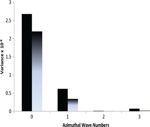
Figure 21 illustrates the variances around the radius 10–20 km for the liquid water mixing ratio for 28 August 1700 UTC when a cloud burst was occurring. These are shown for the azimuthal wave number 0, 1, 2 and 3. Also shown in this illustration are the variances when that single cloud burst was omitted (by setting the liquid water mixing ratios to zero). The bar on the left shows the results when the cloud burst is included and the bar on the right are results when it is removed. It is clear that the hurricane scale (wave numbers 0–2) variances are reduced when the cloud burst is excluded. This suggests that a single cloud burst, in the right place, can contribute to the hurricane scale variances. It should be noted that the scale of individual flare-ups are of the order of 5 km or less. Those flare-ups do not project on to low azimuthal wave numbers. Although cloud flare-ups, appear to be local events around the eye wall, the large variance in wave number 0 shows clearly that the axisymmetric component does acquire an importance during these events. This suggests that these cloud flare-ups can influence the entire storm. The axisymmetric component of the hurricane's response to the scenario of cloud burst and related parameters of this study strongly suggest that these findings may have a strong relationship to the findings of Emanuel (1986, 1988, 1997) and Montgomery (1997). Those deserve further studies.

Fig. 21.  Variances for the azimuthal harmonics 0, 1, 2 and 3 for the case where a cloud element was growing along the inner eye wall (shown by dark bars). Also shown are variances when the liquid water mixing ratio of the cloud element was put to zero.

These illustrations convey an important message for hurricane model initialisation. The fields of GWDs clearly show an organisation, in the azimuthal direction, which is quite similar to that of the radar imagery. This implies that the GWDs are an integral part of the hurricane's life cycle and are very intimately related to the clouds that grow within a hurricane. Hence, an initialisation of the GWDs, rather than a gradient wind balance, is what is required to start off a model forecast properly. This also has important implications for the initial spin up in mesoscale numerical weather prediction of hurricanes.

7. Why the flare-ups?

From the model output, at the 1.33 km resolution and at intervals of every hour, it was possible to see an azimuthal pattern of buoyancy. The buoyancy is defined as follows:10

where r _l is the liquid water mixing ratio, and and, respectively, denote virtual temperature values inside a cloud (where r _l >0.1 g/kg) and outside a cloud (where r _l <0.1 g/kg). The virtual temperature T _v is defined as:

where T denotes air temperature, r _v is the mixing ratio of water vapour and ɛ is the ratio of molecular weights of water vapour and dry air (ɛ=0.622).

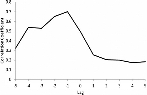
A sequence of four panels in Fig. 22 shows the hourly field of buoyancy (ms⁻²) at the 850 hPa level for 28 August 2005. These are computed from the model output fields. They show that the structure of the buoyancy is somewhat similar to that of the liquid water mixing ratio, but not exactly the same. Regions of large buoyancy move around the storm, clearly from advective effects. When regions of large buoyancy arrive over regions of clouds, as determined from the liquid water mixing ratios, some of these clouds show flare-ups. Figure 23 illustrates the lag correlations (along ordinate) between the buoyancy (at 850 hPa level) and the liquid water mixing ratio (vertically integrated from surface to the 450 hPa level). The abscissa denotes the lag in hours. Minus sign denotes liquid water leading the buoyancy. This illustration shows that the liquid water mixing ratio lead the buoyancy by an hour in this model forecast of hurricane Katrina.

Fig. 22.  The hourly depictions of Buoyancy (ms⁻²) at 850 hPa level. (a) 1500 UTC 28 August 2005; (b) 1600 UTC 28 August 2005; (c) 1700 UTC 28 August 2005; (d) 1800 UTC 28 August 2005.

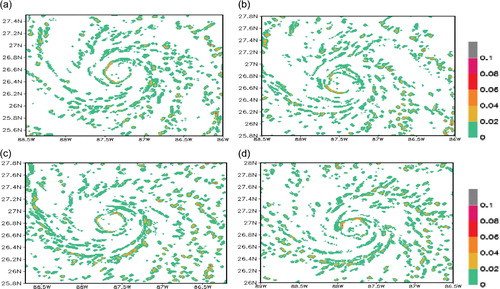
Fig. 23.  Lag correlations (along ordinate) between the buoyancy, at 850 hPa level) and the liquid water mixing ratio (vertically integrated from 950 to the 450 hPa level). The abscissa denotes the lag in hours. Minus sign denotes liquid water leading the buoyancy.

8. Conclusions and future work

In this study, the model output from a hurricane simulation, Davis et al. (2008), at a high horizontal resolution of 1.33 km is utilised to carry out post-processing. The findings show a scenario where cloud flare-ups along the inner eye wall are associated with the local growth of the lower tropospheric convergence, growth of the departures from balance laws and the generation of local supergradient winds. It is also noted that the overall rapid intensification of hurricane Katrina (from the model output) required an organisation of such convection around the inner eye wall for low wave numbers in the azimuthal direction. Growth of isolated deep convection away from the eye wall do not seem to contribute to the azimuthal variances for low wave numbers and, therefore, do not seem to support the above scenario.

An important contribution of this article is the solution of the complete storm-centred radial gradient wind equation, which includes the GWDs; this provides local tangential wind solutions that can be supergradient. That happens wherever these departures are large and negative, and these are a part of the scenario of cloud bursts, divergence, departures from balance laws and the supergradient winds. A collection of several such events along the inner eye wall can contribute to an overall intensification of the hurricane.

The cloud flare-ups in the model were noted to be rather robust features; they contribute to the well-known, near-constant, θe profiles of a hurricane in the vertical. They also augment the surface fluxes of momentum, sensible and latent heat. Furthermore vertical cross sections and time sections of the temperature anomaly show that the cloud burst incidents contribute to the maintenance of the warm core (residing near 250–300 hPa levels) of the hurricane. When the lags of various fields were examined in the context of the flare-up, it was noted that the cloud liquid water leads the buoyancy by about one hour around the inner eye wall. The other parameters such as divergence, GWDs and the maximum winds did not exhibit any perceptible lag with respect to buoyancy. The liquid water mixing ratio carries some elements with large values, and those can be followed on hourly panels of liquid water mixing ratio; it is possible to see buoyancy elements flaring up when large liquid water elements arrive over such regions. Thus a possible scenario for rapid intensification, suggested by this model output, is that strong tangential winds advect strong pockets of liquid water mixing ratio, which in turn enhance the local buoyancy of cloud elements that show a flare up, the scenario of GWDs and the generation of supergradient winds follows. The azimuthally averaged features discussed above also carry some of these signatures.

In that context it is worthwhile stating that the NASA field experiment, Genesis and Rapid Intensification Processes (GRIP), from summer 2010 was designed to provide observations for hurricane intensity studies. During that experiment there were two aircraft deploying WIND LIDAR inside hurricanes. Besides that Rapid Scan winds, i.e. cloud tracked winds, from GOES geostationary satellites were obtained. The aircraft, along with a plethora of dropwindsondes, provided as many as several thousand wind vectors in three dimensions in the inner core of the observed hurricanes. Several of these aircraft carried radar to monitor the radar reflectivity. Thus we expect to carry out an observational validation of the aforementioned scenario of cloud bursts leading to rapid intensification using the GRIP data.

This article addresses only one small aspect of the hurricane intensity issue. Research on this topic has increased considerably in recent years. There is a broad range of issues that are being considered for the rapid intensity changes of a hurricane. The ongoing research by the community of scientists will eventually address all of the issues for a coherent understanding of hurricane intensity and its changes.

The prediction of rapid intensification is a difficult issue even for mesoscale models that carry a high enough resolution to resolve the inner core of hurricanes. Mesoscale models carry many uncertainties that arise from data problems, data assimilation, lateral boundary conditions, parameterisation of physical and microphysical processes, treatment of the upper oceans and the handling of aerosols such as dust. There are a host of basic fields and derived variables that seem to provide some clues for possible intensity changes over short periods of time. These include the well-cited parameters such as the wind shear, warm SST anomalies, heat content of the upper ocean and intrusions of dust and dry air into the inner core. These fields are routinely examined during operational forecasts by the National Hurricane Center. In addition to these there are other promising parameters that can be derived from the model's initial fields that could provide short range guidance for rapid intensity changes. Examining these parameters over the lower troposphere, Simon et al. (2010) noted, from an examination of all of the hurricanes during a three-year period, that rapid intensity changes were related to the growth or decay of these parameters. To these we can add the cloud bursts and growth of departures from balance laws as yet another possible parameter. These fields are presently being calculated from model assimilated fields; the model itself, because of the deficiencies, is not able to predict rapid intensity changes. Thus, as future work, we suggest the possible use of statistical techniques, where the intensity changes could be related to the base fields and to the parameters such as those cited above and their time rates of changes as well. Prior to the further advancements of mesoscale modelling such an approach may prove useful for the prediction of short-term rapid intensity changes.

Acknowledgements

This research has been supported by NASA grant NNX09AC37G.

10. Appendix

By starting from the equation of motion:A1

where Φ=gh, is the geopotential and F denotes the frictional force per unit mass, one forms the complete divergence (D) equation,A2

where V _ψ, V _χ are the rotational and divergent winds.

If we start with the assumption that the divergent part of the wind is zero then we obtain the balance equation:A3

where ψ is the stream function.

If we now go back to eq. (A1) and transform the scalar horizontal velocity components u, v to a local storm-centred cylindrical coordinate about a reference location of storm centre x ₀, y ₀, we obtain a complete radial equation of motion:A4

The local gradient wind balance in storm-centred coordinates retain the formA5

This is obtained by the same approximation as are used in deriving the non-linear balance equation (A3). Since eqs. (A3) and (A5) both represent balance under the constraint of non divergence they bear a relationship to each other.

References

- Bender M. A. Ginis I. Tuleya R. Thomas B. Marchok T. The operational GFDL coupled hurricane–ocean prediction system and a summary of its performance. Mon. Wea. Rev. 2007; 135: 3965–3989. 10.3402/tellusa.v64i0.18399.
- Braun S. A. Tao W. K. Sensitivity of high-resolution simulations of Hurricane Bob (1991) to planetary boundary layer parameterizations. Mon. Wea. Rev. 2000; 128: 3941–3961. 10.3402/tellusa.v64i0.18399.
- Carlson T. N. Boland F. E. Analysis of urban-rural canopy using a surface heat flux/temperature model. J. Appl. Meteor. 1978; 17: 998–1013. 10.3402/tellusa.v64i0.18399.
- Charnock H. Wind stress on a water surface. Quart. J. Roy. Meteor. Soc. 1955; 81: 639–640. 10.3402/tellusa.v64i0.18399.
- Davis, C, Wang, W, Chen, S. S, Chen, Y, Corbosiero, K and co-authors. 2008. Prediction of landfalling hurricanes with the advanced hurricane WRF model. Mon. Wea. Rev. 136, 1990–2005. 10.3402/tellusa.v64i0.18399.
- Emanuel K. A. An air–sea interaction theory for tropical cyclones. Part I: steady-state maintenance. J. Atmos. Sci. 1986; 43: 585–604. 10.3402/tellusa.v64i0.18399.
- Emanuel K. A. The maximum intensity of hurricanes. J. Atmos. Sci. 1988; 45: 1143–1155. 10.3402/tellusa.v64i0.18399.
- Emanuel K. A. Some aspects of hurricane inner-core dynamics and energetics. J. Atmos. Sci. 1997; 54: 1014–1026. 10.3402/tellusa.v64i0.18399.
- Fankhauser J. C. The derivation of consistent fields of wind and geopotential height from mesoscale rawinsonde data. J. Appl. Meteor. 1974; 13: 637–646. 10.3402/tellusa.v64i0.18399.
- Gopalakrishnan, S. G, Marks, F, Zhang, X, Bao, J.-W, Yeh, K.-S and co-authors. 2011. The experimental HWRF system: a study on the influence of horizontal resolution on the structure and intensity changes in tropical cyclones using an idealized framework. Mon. Wea. Rev. 139, 1762–1784. 10.3402/tellusa.v64i0.18399.
- Haltiner G. J. Williams R. T. Numerical Weather Prediction and Dynamic Meteorology. John Wiley and Sons.1980; 477.
- Hawkins H. F. Imbembo S. M. The structure of a small, intense hurricane, Inez. Mon. Wea. Rev. 1976; 99: 427–434. 10.3402/tellusa.v64i0.18399.
- Hennon, P. A. 2006. The role of ocean in convective burst: implications for tropical cyclone intensification. PhD Dissertation, Graduate School, Ohio State University.
- Hong S.-Y. Dudhia J. Chen S.-H. A revised approach to ice microphysics process for the bulk parameterization of clouds and precipitation. Mon. Wea. Rev. 2004; 132: 103–120. 10.3402/tellusa.v64i0.18399.
- Jaimes B. Shay L. K. Mixed layer cooling in mesoscale oceanic eddies during hurricanes Katrina and Rita. Mon. Wea. Rev. 2009; 12: 4188–4207. 10.3402/tellusa.v64i0.18399.
- Kain J. S. The Kain–Fritsch convective parameterization: an update. J. Appl. Meteor. 2004; 43: 170–181. 10.3402/tellusa.v64i0.18399.
- Kain, J. S and Fritsch, J. M. 1993. Convective parameterization for mesoscale models: The Kain–Fritsch scheme. The representation of cumulus convection in numerical models. Amer. Meteor. Soc. Meteor. Monogr., No. 24, . 165–170.
- Knabb, R. D, Brown, D. P and Rhome, J. R. 2005. Tropical cyclone report Hurricane Katrina 23–30 August 2005. NCEP Rep. In National Hurricane Center, Miami, Florida. Online at: http://www.nhc.noaa.gov/pdf/TCR-AL122005_Katrina.pdf.
- Krishnamurti T. N. A diagnostic balance model for studies of weather systems of low and high latitudes, Rossby numbers less than. Mon. Wea. Rev. 1968; 96: 197–207. 10.3402/tellusa.v64i0.18399.
- Krishnamurti, T. N, Pattnaik, S, Stefenova, L, Vijayakumar, T. S. V, Mackey, B. P and co-authors. 2005. On the hurricane intensity issue. Mon Wea Rev. 133, 1886–1912. 10.3402/tellusa.v64i0.18399.
- Mainelli M. M. DeMaria M. Shay L. K. Goni G. Application of oceanic heat content estimation to operational forecasting of recent Atlantic Category 5 Hurricanes. Wea. Forecasting. 2008; 23: 3–16. 10.3402/tellusa.v64i0.18399.
- McFarquhar G. M. Black R. A. Observations of particle size and phase in tropical cyclones: implications for mesoscale modeling of microphysical processes. J. Atmos. Sci. 2004; 61: 422–439. 10.3402/tellusa.v64i0.18399.
- McTaggart-Cowan R. Bosart L. F. Gyakum J. R. Atallah E. H. Hurricane Katrina 2005. Part I: complex life cycle of an intense tropical cyclone. Mon. Wea. Rev. 2007a; 135: 3905–3926. 10.3402/tellusa.v64i0.18399.
- McTaggart-Cowan R. Bosart L. F. Gyakum J. R. Atallah E. H. Hurricane Katrina 2005. Part II: evolution and hemispheric impacts of a diabatically generated warm pool. Mon. Wea. Rev. 2007b; 135: 3927–3949. 10.3402/tellusa.v64i0.18399.
- Montgomery M. T. Enagonio J. Tropical cyclogenesis via convectively forced vortex Rossby waves in a three-dimensional quasigeostrophic model. J. Atmos. Sci. 1998; 55: 3176–3207. 10.3402/tellusa.v64i0.18399.
- Montgomery M. T. Kallenbach R. J. A theory for vortex Rossby waves and its application to spiral bands and intensity changes in hurricanes. Quart. J. Roy. Meteor. Soc. 1997; 123: 435–465. 10.3402/tellusa.v64i0.18399.
- Nguyen V. S. Smith R. K. Montgomery M. T. Tropical cyclone intensification and predictability in three dimensions. Quart. J. Roy. Meteor. Soc. 2008; 134: 563–582. 10.3402/tellusa.v64i0.18399.
- Noh Y. Cheon W. G. Hong S. Y. Raasch S. Improvement of the K-profile model for the planetary boundary layer based on large eddy simulation data. Bound.-Layer Meteor. 2003; 107: 421–427. 10.3402/tellusa.v64i0.18399.
- Pattnaik S. Krishnamurti T. N. Impact of cloud microphysical processes on hurricane intensity, part 1: control run. Meteorol. Atmos. Phys. 2007a; 97: 117–126. 10.3402/tellusa.v64i0.18399.
- Pattnaik S. Krishnamurti T. N. Impact of cloud microphysical processes on hurricane intensity, part 2: sensitivity experiments. Meteorol. Atmos. Phys. 2007b; 97: 127–147. 10.3402/tellusa.v64i0.18399.
- Phillips, N. A. 1963. Geostrophic Motion. Reviews of Geophysics. WashingtonDC, 1 ( 2), 123–176.
- Powell M. D. Houston S. H. Surface wind fields of 1995 Hurricanes Erin, Opal, Luis, Marilyn, and Roxanne at landfall. Mon Wea. Rev. 1998; 126: 1259–1273. 10.3402/tellusa.v64i0.18399.
- Powell M. D. Houston S. H. Amat L. R. Morisseau-Leroy N. The HRD real-time hurricane wind analysis system. J. Wind Engineer. Indust. Aerodyn. 1998; 77&78: 53–64. 10.3402/tellusa.v64i0.18399.
- Rogers R. F. Black M. L. Chen S. S. Black R. A. An evaluation of microphysics fields from mesoscale model simulations of tropical cyclones. Part I: comparisons with observations. J. Atmos. Sci. 2007; 64: 1811–1834. 10.3402/tellusa.v64i0.18399.
- Simon A. Krishnamurti T. N. Ross R. Martin A. Relationship of rapid intensification of tropical cyclones to dynamical/thermodynamical parameters. Marine. Geodesy. 2010; 33: 4.10.3402/tellusa.v64i0.18399.
- Skamarock, W. C, Klemp, J. B, Dudhia, J, Gill, D. O, Barker, D. M and co-authors. 2005. A description of the Advanced Research WRF version 2. NCAR Tech. Note TN-468+STR, 88.
- Smith R. K. Montgomery M. T. Balanced boundary layers used in hurricane models. Q. J. R. Meteorol. Soc. 2008; 134: 1385–1395. 10.3402/tellusa.v64i0.18399.