Simultaneous global and limited-area ensemble data assimilation using joint states

ABSTRACT

We propose a data assimilation scheme that simultaneously produces the analyses for a global model and an embedded limited-area model, considering forecast information from both models. The purpose of the proposed approach is twofold. First, we expect that the global analysis will benefit from incorporation of information from the higher resolution limited-area model. Second, our method is expected to produce a limited-area analysis that is more strongly constrained by the large-scale flow than a conventional limited-area analysis. The proposed scheme minimises a cost function in which the control variable is the joint state of the global and the limited-area models. In addition, the cost function includes a constraint term that penalises large differences between the global and the limited-area state estimates. The proposed approach is tested by idealised experiments, using ‘toy’ models introduced by Lorenz in 2005. The results of these experiments suggest that the proposed approach improves the global analysis within and near the limited-area domain and the regional analysis near the lateral boundaries. These analysis improvements lead to forecast improvements in both the global and the limited-area models.

• ensemble data assimilation
• ensemble Kalman filter
• joint states
• limited area
• Lorenz model

1. Introduction

We consider data assimilation in the scenario where we have a global model and a limited-area model, which more accurately represents some smaller scale processes, defined in a subregion inside the global region. We aim to produce analyses for both the global and the limited-area models by a single data assimilation process using information from both models. We hope that both the global and the limited-area forecast accuracy will benefit from estimating the initial state of the two models jointly. Our proposed method, which we call the ‘joint-state method’, is based on introducing an observation function and a cost function that both depend on the joint state. The minimiser of this cost function, which provides the analysis for both models, can be found using either a variational or a sequential algorithm. Our proposed scheme would most likely be of potential interest for centres where both global and limited-area forecasts and analyses are prepared.

Similar previous attempts in the literature (Guidard and Fischer, 2008; Dahlgren and Gustafsson, 2012) focused on the narrower objective of propagating information from a pre-computed global analysis into the limited-area data assimilation process, not only through the lateral boundary conditions but also by imposing a constraint on the limited-area analysis of the large-scale features of the atmospheric flow inside the limited-area domain. The motivation for those efforts was the general experience of the numerical weather prediction centres that a limited-area analysis provides a lower quality representation of the large-scale features of the atmospheric flow (e.g. baroclinic waves) than the host global analysis, which provides the lateral boundary conditions for the limited-area model. This behaviour of the limited-area analysis is usually explained by the effects of aliasing the large-scale information contained in the observations on the shorter scales present in the limited-area analysis; the inability of the limited-area analysis systems to gainfully assimilate satellite radiance observations, due to the lack of efficient strategies for observation bias correction in the limited-area setting; and the effects of ignoring the observations outside the limited-area domain [a review of the different techniques that have been considered by the different authors for imposing a large-scale constraint based on the global analysis on the limited-area analysis can be found in Guidard and Fischer (2008)].

The new aspect of our approach is that the global analysis is prepared simultaneously with the limited-area analysis, that is, the limited-area model information can affect the global analysis. As will be shown, this approach leads to improvements, not only in the limited-area analysis but also in the global analysis. To our knowledge, the only data assimilation system that uses higher resolution model information from an inner limited-area domain is the Data Assimilation Research Testbed implementation of the Weather Research and Forecasting Model (WRF/DART; Anderson et al., 2009). In that system, the state at a given location is represented by the highest resolution nest available at that location and the analysis for the lower resolution outer nests is obtained by an interpolation of the higher resolution analysis to the lower resolution grid of the outer nests (personal communication; Chris Snyder, 2012). Such analyses can be used as the initial conditions of two-way nested limited-area weather forecasts, which have been shown to have major benefits even for such challenging forecast problems as the prediction of the intensity of tropical cyclones (Zhang et al., 2011). The algorithm we propose could also be extended to prepare an analysis for a limited-area system using multiple nests. The simple approach used by WRF/DART can be considered a special case of such an extension.

To test our global/regional assimilation technique, we design a global/regional forecast system based on two ‘toy’ models proposed by Lorenz (2005). We obtain analyses for the toy model system by finding the minimiser of the cost function with the help of the Local Ensemble Transform Kalman Filter (LETKF) algorithm, which was proposed by Ott et al. (2004) and Hunt et al. (2007). The LETKF algorithm, like other localisation methods, makes use of the assumed locality of atmospheric interactions and, on that basis, performs and combines analyses in relatively small overlapping regions. This greatly facilitates numerical data assimilation. While the ‘toy’ model system that we use mimics the realistic situation in a way that is overly simplified in many respects, it allows for a speedy code development and the execution of a large number of numerical experiments, which would not be possible with a more realistic system. We note that the LETKF scheme, similar to other ensemble-based data assimilation schemes that have been successfully implemented on operational models (e.g. Whitaker and Hamill, 2002), was initially tested on the toy model called model 1 in Lorenz (2005).

We compare the accuracy of the analyses and forecasts obtained by our joint-state method and the accuracy of the global and limited-area analyses and forecasts that were obtained separately. Hereafter, we refer to the latter approach as separate analysis method. We find that better forecasts are produced using the joint-state method than the separate analysis method. While this positive result with the toy model does not guarantee that our approach will work in a realistic setting, we believe that it is sufficiently encouraging to make the significant investment of effort required by an implementation on a realistic system in the near future.

The organisation of the article is the following. Section 2 introduces the atmospheric toy models that we use. Section 3 describes the data assimilation schemes by the joint-state method and the separate analysis method. Section 4 describes how the regional model is coupled to the global model at the boundaries of the subregion during the integration phases of analysis cycles, and how we choose some parameter values of the system. Section 5 compares the results of our joint-state method to those of the separate analysis method. Section 6 shows the dependence of the analysis errors of our joint-state method on its parameters, with and without model error. Section 7 gives further discussion and summarises our conclusions.

2. True model, global model and regional model

Lorenz (2005) introduced three simple, spatially discrete, one-dimensional models that have proven to be useful for testing weather data assimilation methods. Here, we will use Lorenz model 2 (which shows smooth propagating waves) and the more refined Lorenz model 3 (which shows small-scale activities on top of smooth waves). Lorenz model 3 is the following equation for the evolution of a scalar state variable Z _n at spatial location n,1

where n is an integer, n=0, 1,…, N−1, t is time, K, b, c and F are parameters, and a periodic boundary condition (Z _N =Z₀) is used. The convention of index counting starting from 0 is used throughout this article. N-component vectors X and Y are defined as2 3 4 5

where the prime notation on Σ′ signifies that the first and the last terms in the summation are divided by two, and I is a parameter. The bracket of any two vectors X and Y is defined as6

when K is even, and Σ′ is replaced by Σ when K is odd; J=K/2 when K is even, and J=(K−1)/2 when K is odd. Model 3 reduces to model 2 when I=1. In particular, for I=1, eq. (2) yields X _n =Z _n , which by eq. (3) implies that Y _n =0. Thus, after changing notation, n→m and Z _n →Z _m , we obtain7

where m is used to denote a point on the coarser grid of the global model. Lorenz (2005) defined 5 d to be the time unit in the equations considering the damping time. We follow this convention in this article.

We use Lorenz model 3 with parameter values N=960, K=32, b=10, c=0.6, F=15 and I=12 to generate our simulated true dynamics, and Lorenz model 2 with N=240, K=8, F=15 for the global model defined at every fourth grid point of the true model (n=0, 4, 8, …, 956). Thus, the grid points for eq. (7) occur at m=n/4, where n=0, 4, 8, …, 956. Note that like Lorenz (2005) we kept N/K to be 30 to make roughly 7 waves in both model 3 and model 2. We assume that, between analyses, eq. (7) for Z _m gives an approximation of the dynamical evolution of Z _n (t) at the grid points n=4m. When referring to locations or lengths of regions, we use the coordinate system of the true model throughout this article (n=0, 1, …, 959). For the regional model, we define a subregion extending from n=n ₀=240 to n=n ₁=720 grid and use Lorenz model 3 with the same parameter values as the true model. To integrate this regional model, we must evaluate the bracket quantities on the right hand side of eq. (1) defined by eq. (6). For n too close to n ₀ (n ₁), this involves X, Y and Z values at grid points outside the subregion, n<n ₀(n>n ₁). Also, from eq. (2), X _n in the regional model (and hence also Y _n ) depends on Z _n′ values in n′<n ₀(n′>n ₁) if n is within a distance I of n ₀ (n ₁). To evaluate these quantities, we use estimates of the required values of Z _n′ obtained from linear interpolation of the global values Z _m onto the n-grid. These interpolations essentially play the role of boundary conditions for the regional model.

The spatiotemporal average of the ‘true’ state is about 2.75, whereas the spatiotemporal average of the global model state is about 2.73. In addition, the spatiotemporal average of the state of the regional model (coupled to the global model) is about 2.83. (The global model bias is less than 1%, whereas the regional model bias is less than 3%.) These numbers suggest that we can expect model bias to make only a small contribution to the state estimation error, especially in the case of the global model. Thus, the primary role of the state-update step of the data assimilation will be to correct transient errors in the background.

3. Data assimilation

We selected 15 evenly spaced observation points starting from n=0 (n=0, 64, 128, …, 896). Note that all the observation points are at grid points defined in the global model. We construct simulated observations by adding random noise drawn from independent Gaussian distributions of standard deviation 1 to the true state values at the observation points. The standard deviation 1 of the observational noise can be compared with the standard deviation 5.7 of the climatological distribution of the true state.

We compare two data assimilation methods. The first method does data assimilation for the global model and the regional model separately, whereas the second method, which we call the joint-state method, forms a combined state from the global model and the regional model and does data assimilation on the combined state. The intuition motivating our second method is that we expect the global and the regional estimates will both benefit from information exchange between them. We use LETKF for both methods. See Hunt et al. (2007) for an explanation of LETKF.

For the separate analysis method, we use LETKF without much modification. For the global analysis, at each grid point n=4m defined in the global model, we define a local patch [n−s, n+s] of size 2s+1 regional grid points, where for this article we use s=40. We use the Ensemble Transform Kalman Filter (ETKF) to obtain an analysis for the 2s/4+1=21 global state values in each patch. This yields local patch analyses for each ensemble member. As done by others (e.g. Hunt et al., 2007), we then use these patch analyses to form the global analysis states for each ensemble member by defining the value of the global ensemble field at each point m=n/4 to be the analysis state value of that ensemble member in the centre of patch n=4m. For the regional analysis, at each grid point n defined in the regional model, we define a local patch, limiting the size near the two boundaries of the subregion so that the local patch is defined only inside the subregion, use ETKF and take the patch analysis value at grid point n. Thus, the global local patches always have size 2s+1, but the regional local patches have variable sizes depending on n. For n located in the subregion and also far away from the boundaries, the regional local patch has size 2s+1, whereas for n near the boundaries (n+s>n ₁ or n−s<n ₀), the regional local patch is the intersection, , and has a size less than 2s+1.

For the joint-state method, we use the same local patch size, s=40. For each grid point n defined either in the global model or in the regional model, we define a global local patch and a regional local patch (where, as before, the regional patch is the intersection, , which for some n=4m will be empty). For each such grid point n, we define a vector by taking state values of the global local patch and by taking state values of the regional local patch, and we then form a local joint-state vector x ⁽ⁿ⁾ by concatenating and , i.e.8

We also form a local observation vector by taking observations in the local patches (from grid point n–s to n+s).

We seek an analysis that, in the subregion, combines the global state, the regional state and the observations. It is not possible to constrain all three fields to be close to each other with a single quadratic term in the cost function that the analysis minimises. Three-way coupling can be achieved in a variety of ways; we choose to include a term that couples a linear combination of the global and regional states to the observations, and a term that couples the global and regional states to each other. Specifically, we define a local cost function J ⁽ⁿ⁾( x ⁽ⁿ⁾) for grid point n as follows,9

where and are the local mean and the covariance matrix of the background ensemble, respectively, and R is the covariance matrix of the observation noise. H ⁽ⁿ⁾( x ⁽ⁿ⁾) is a local observation operator defined as10

where j(i) is the observation location of the i ^th observation in the local patch, x _g,j(i) is the global state value at location j(i), and x _r,j(i) is the regional state value at location j(i). is a vector that consists of the state values of the global state at the grid points defined both in the global and the regional local patches. Similarly, is a vector that consists of the state values of the regional state at the grid points defined both in the global and the regional local patches. Furthermore, κ and λ are parameters. We remark that the WRF/DART approach corresponds to the special case κ=0 and λ=1, with the state in the outer nest replacing the state of the global system. However, we found that when κ=0, the global state tends to diverge from the regional state in the middle of the local region. To be effective, the value of κ should make the magnitude of the third term in the cost function comparable to the other two terms. In this sense, we can think of κ as having units of an inverse variance, but in practice we determine the value of κ by tuning.

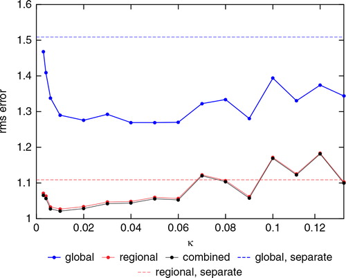
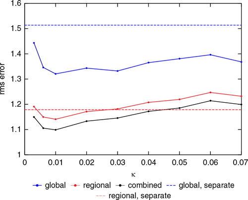
Fig. 4.  Rms analysis error versus κ. λ is fixed at 0.9. The blue, red and black curves show the global, regional and combined rms errors, respectively. The blue and red horizontal dashed lines show the global and the regional rms errors from the separate analysis method. The values were averaged over 40 000 analysis cycles discarding the first 1000 cycles.

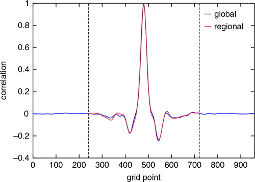
Fig. 7.  Rms analysis error versus κ with λ =0.7. A model error was introduced to the regional model by using F=14 in Lorenz model 3. The blue and red horizontal dashed lines show the global and the regional rms errors from the separate analysis method. The values were averaged over 80 000 analysis cycles discarding the first 1000 cycles.

The cost function of Guidard and Fischer (2008) is similar to ours, except that their control variable is the state of the limited-area model instead of the joint state. An equally important difference between their approach and ours is that we determine the value of x ⁽ⁿ⁾ that minimises the cost function J ⁽ⁿ⁾( x ⁽ⁿ⁾) with the LETKF algorithm (Hunt et al., 2007), whereas they use an incremental variational approach. The advantage of the ensemble-based approach is that it automatically accounts for the covariance between the uncertainties in the estimates of the global and the limited-area states, whereas the variational approach requires making strong assumptions about the covariance. The trade-off we take is that the estimate of all covariances, including the covariances between the different components of the limited-area state and between the different components of the global state, are limited to the low-dimensional state spanned by the ensemble perturbations in the ensemble-based approach, whereas a variational approach can seek the minimiser in a much higher dimensional space.

In general, if our technique were to be applied in an operational setting, the grid points of the global and the regional models within the subregion will not coincide. In that case, to calculate the third term in J ⁽ⁿ⁾( x ⁽ⁿ⁾), an interpolation from the grid points of the regional model to the grid points of the global model or vice versa could be employed before the values of the regional and the global models are subtracted. Similarly, in an operational setting, the observations are not at grid points, and H ⁽ⁿ⁾ would then include interpolation, and R would include a representativeness error component (Lorenc, 1986).

4. Implementation of the joint-state method for Lorenz models

We define a smoothed regional state for the initial condition of the regional model for integration between analysis times as follows. After the analysis phase, we define spatial transition intervals of length 10 starting from the boundaries and ending inside the subregion. We then modify the regional analysis values in the transition intervals by taking weighted linear averages of the global analysis values and the regional analysis values. We do this to make the transition between the global model and the regional model smooth at the boundaries. A similar approach is often used in the form of a ‘sponge region’ in limited-area models. For n such that 0≤n<10, we modify the regional ensemble members by11 12

where and are the values of the k ^th global and regional ensemble members at grid point n, respectively. The global state values are linearly interpolated to the fine grid points of the regional model in this sponge region. The subregion for the regional model is [n ₀, n ₁]=[240, 720].

After performing the above smoothing process, we integrate each global and regional ensemble member for 6 h using a fourth-order Runge-Kutta method, dividing 6 h into 48 time steps. We integrate the global ensemble members independent of the regional ensemble members. For the integration of the regional ensemble members, we use the necessary interpolated values of the corresponding global ensemble members outside the subregion at each Runge-Kutta time step to synchronise the global and the regional model at the boundaries.

Before we tested the joint-state method and the separate analysis method, we ran analysis cycles with 40 ensemble members using the global and the regional models separately and found that multiplicative covariance inflation factors of 0.024 and 0.02 for the global and the regional analyses, respectively, produce the lowest rms state estimate errors. We henceforth use these values in our data assimilations. For the joint-state method, we found that λ=0.9 and κ=0.04 in eqs. (9) and (10) give relatively low rms state estimate errors compared to other combinations of values for λ and κ, and use these values for the joint-state method in this section. Section 6 shows the parameter dependence of the rms errors.

Finally, we assess the length scale of background error correlations by calculating the climatological (time-averaged) correlations of the background ensemble of the joint-state method without localisation at each grid point with respect to the middle grid point of the limited-area domain. Fig. 1 shows the correlation values averaged over 20 000 analysis cycles using 720 ensemble members as a function of the grid point.

Fig. 1.  Correlations of the background ensemble of the joint-state method without localisation as a function of the grid point. Seven hundred and twenty ensemble members were used. The values were averaged over 20 000 analysis cycles.

The blue and red curves show the correlation structures of the global and the regional background ensembles, respectively. The figure shows that the climatological correlation length is similar for the two systems and is smaller than the size of the limited-area domain. Based on the correlation length of the figure, we use the local patch size of 2×40+1 for the localisation.

5. Space dependence of the rms error

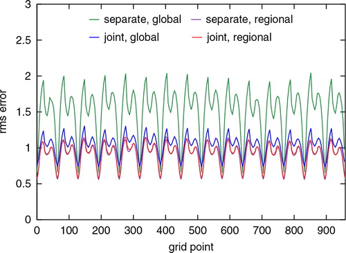
Among the effects that the joint-state method has relative to the separate analysis method are: (1) the global analysis is influenced by the comparison of the higher quality regional background to the observations and (2) the regional analysis is directly affected by observations outside the subregion during the analysis cycle, not just via the coupling with the global model during the forecast step. To assess separately effect (1), we first tested the separate analysis method and the joint-state method without boundaries. That is, we used the whole region for both the global and regional models. Thus, there is no coupling between the global model and the regional model at the boundaries during the integration phases. Then for the separate analysis method, the data assimilation cycles for the two models are completely independent, except that they use the same observations. For the joint-state method, the coupling between the global and regional models occurs only at the analysis phases. Figure 2 shows the rms errors of state estimates given by the means of the ensemble members as a function of the grid point.

Fig. 2.  Rms analysis errors of the separate analysis and the joint-state analysis using the whole region for both the global and the regional models. In this and the subsequent figures, the rms error values were averaged over enough cycles to give stable values. In the case of present figure, the rms-error values were averaged over 100 000 analysis cycles, discarding the values of 1000 initial cycles. The green and the purple colours correspond to the global and the regional values obtained using the separate analysis method. The blue and the red colours correspond to the global and the regional values obtained using the joint-state method. The purple and the red lines are close to each other.

The values were averaged over 100 000 analysis cycles, discarding the values of 1000 initial cycles. The green and the purple colours correspond to the global and the regional values obtained from the separate analysis method. The blue and the red colours correspond to the global and the regional values obtained from the joint-state method. Error minima occur at the observation points. The figure shows that the two regional rms errors are almost the same, whereas the global rms errors from the joint-state method are much lower than the global rms errors of the separate analysis case indicating that, as one would expect, the information from the regional model substantially improved the estimate of the global model.

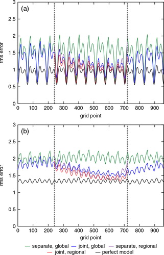
Now, we take a subregion [n ₀, n ₁]=[240, 720] and introduce coupling between the global model and the regional model at the two boundaries during the integration phase. Figures 3(a) and 3(b) show the rms errors of the analysis and of a 1-d forecast, respectively, using the same colour scheme as in Fig. 2.

Fig. 3.  Rms errors of (a) the analysis (b) 1 d forecast of the separate analysis and the joint-state analysis. The colour scheme is the same as in Fig. 2. The additional black curves show the rms-error values when assimilations were done globally using the true model (Lorenz model 3). The two vertical dashed lines at grid points 240 and 720 indicate the boundaries of the subregion. The rms-error values were averaged over 100 000 analysis cycles.

The two vertical dashed lines at grid points 240 and 720 indicate the boundaries of the subregion. As a baseline, the additional black curves show the rms-error values in the perfect model scenario in which the forecast model was the true model (Lorenz model 3) which was used globally throughout the entire space. We view this as setting a standard for the best that could ever be done. These figures show that the joint-state method performs better than the separate analysis method for both global and regional predictions. We note that the global forecast obtained from the joint-state method is better than the corresponding one from the separate analysis method even outside the subregion. This can be explained by the fact that the better global state estimates inside the subregion at the analysis phases can make better forecasts outside the subregion during the integration phases, and these better forecasts outside the subregion can make the regional forecasts better inside the subregion by providing better information at the boundaries during the integration phases. We also note that the global analysis improvements that result from the use of the joint-state method are greater to the right of the subregion than to its left. This is consistent with the fact (Lorenz, 2005; Yoon et al., 2010) that, for these models, waves (and hence the information they carry) have group velocities that are predominantly rightward.

We also computed the rms analysis and forecast errors by replacing temporal averaging by spatiotemporal averaging over the global and in the limited-area domains for the global system, and in the limited-area domain for the regional system. For this error statistic, the joint-state method reduces the analysis error by 18% over the global domain and by 24% in the limited-area domain for the global analysis, and by 6% for the regional analysis. The related error reductions for the ‘1 d’ forecast are, respectively, 15%, 19% and 5%. These numbers suggest that the global analysis and forecast benefit more than the limited-area analysis and forecast from the joint-state approach. In addition, the analysis improvement leads to a ‘1 d’ forecast improvement that is only slightly smaller in magnitude than the analysis improvement.

6. Parameter dependence of the rms error

We now investigate the κ and λ dependencies of the rms errors, averaged over both space and time, of the analysis ensemble mean. Figure 4 shows the global, regional and combined rms errors as a function of κ varying from 0.003 to 0.13 when λ is fixed at 0.9. The global rms errors were calculated at all the grid points of the global model. The regional rms errors were calculated at all the grid points of the regional model. The combined rms errors were calculated over the subregion only, using the linear combination in the observation operator eq. (10), applied to the analysis means (with the global mean interpolated to the regional model grid). The values were averaged over 40 000 analysis cycles discarding the first 1000 cycles. The figure shows that the rms error has a broad minimum roughly lying in the range 0.01<κ<0.06. The regional ensemble blew up during the forecast step before 40 000 cycles, when κ was less than 0.003.

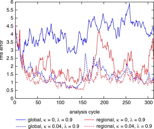
Figure 5 shows the global and the regional rms errors as a function of the analysis cycle when κ=0, λ=0.9 and when κ=0.04, λ=0.9 just before the forecast step for regional ensemble with κ=0 failed at cycle 314. By this time, the global and regional states had become decorrelated at the boundaries, and the regional model integration diverged. The figure shows that the global rms errors with κ=0 are as bad as the rms errors when the true state is estimated by a random climatological state, suggesting that the introduction of the κ-term in the cost function is essential in the joint-state method.

Fig. 5.  Rms analysis error versus analysis cycle. The solid blue and red correspond to the global and the regional rms errors when κ=0, λ=0.9. The dashed blue and red correspond to the global and the regional rms errors when κ=0.04, λ=0.9.

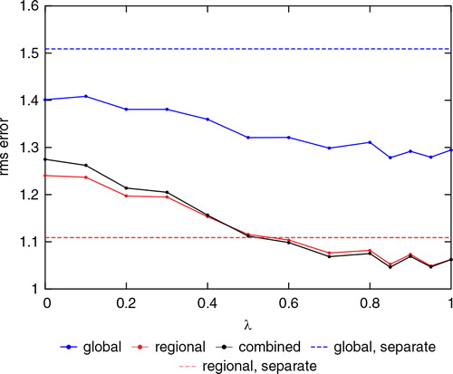
Figure 6 shows the global and the regional rms errors as a function of λ varying from 0 to 1 when κ is fixed at 0.04. The figure shows that the rms errors decrease as λ increases in general, but this pattern is not clear when the range of λ is from 0.8 to 1.

Fig. 6.  Rms analysis error versus λ. κ is fixed at 0.04. The blue, red and black curves show the global, regional and combined rms errors, respectively. The blue and red horizontal dashed lines show the global and the regional rms errors from the separate analysis method. The values were averaged over 200 000 analysis cycles discarding the first 1000 cycles.

Since the regional model is identical to the model generating the ‘truth’ in our results thus far, it is not surprising that values of λ near 1 are optimal. To illustrate that values of λ significantly less than 1 can be advantageous in the presence of model error, we consider a case where the regional model has an error in the large-scale forcing. We introduced such an error by using F=14 in Lorenz model 3 for the regional model (compared with F=15 used for the truth run). Figure 7 shows the global, regional and combined rms errors as a function of κ with λ=0.7. The figure shows that the minimum rms errors occur around κ=0.01.

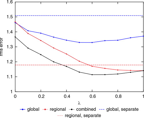
Figure 8 shows the global, regional and combined rms errors as a function of λ with κ=0.01. The figure shows that the minimum global, regional and combined rms errors occur around λ=0.6, 1.0 and 0.6, respectively. This suggests that in the presence of regional model error, using a linear combination of the global and the regional model states as in eq. (10) is better able to fit the observations than the regional state alone (λ=1) and results in better global analyses.

Fig. 8.  Rms analysis error versus λwith κ=0.01. A model error was introduced to the regional model by using F=14 in Lorenz model 3 for the regional model. The blue and red horizontal dashed lines show the global and the regional rms errors from the separate analysis method. The values were averaged over 200 000 analysis cycles discarding the first 1000 cycles.

To investigate the robustness of our results on the reduction of the rms analysis and forecast errors due to the joint-state approach, which we presented at the end of section 5, we compute the same statistics for the case where model error is present. The reduction of the error is 10% over the global domain and 14% in the limited-area domain for the global analysis, and 3% for the limited-area analysis. The same numbers for the ‘1 d’ forecasts are, respectively, 8%, 11% and 4%. While the presence of model error leads to a reduction of the analysis and forecast improvements, the general conclusions are the same as for the model-error-free case: the error reduction is larger for the global than the limited-area system and the reduction in the ‘1 d’ forecast error is comparable to that in the analysis (even slightly larger for the limited-area system).

7. Discussion and conclusion

In this article, we formulated a joint-state method for regional forecasting. Using simulations employing simple models, we have numerically tested our method by comparing analysis and forecast results obtained using our method with results obtained using a separate analysis method. We found that the global analysis and forecast in the whole region and the regional analysis and forecast in the subregion are both noticeably improved when the joint-state method is used compared to when the separate analysis method is used. The improvements are larger for the global than the limited-area system.

We also studied the κ and λ dependence of the rms error from the joint-state method with and without a regional model error. We found that a value of κ greater than 0 is necessary to keep the global and regional states synchronised. Our results suggest that values of λ between 0.5 and 1 are most appropriate, and that values of λ less than 1 can be advantageous when there is error in both the global and the regional models.

This work suggests several topics for future work. Most important, will the encouraging results from experiments using our Lorenz model set-up continue to apply when tests on real situations are done? What are the benefits of applying our coupled analysis scheme to situations with multiple (perhaps overlapping) regional analyses? What is the optimal formulation of the observation operator and the constraint term in a realistic setting? In particular, how should one handle an observation operator that is not a simple linear interpolation in space (e.g. an observation operator for a satellite radiance)? Is it beneficial to filter the smaller scales from the states in the constraint terms, similar to the approach of Guidard and Fischer (2008), or to include only the vorticity components of the state vector, similar to the approach of Dahlgren and Gustafsson (2012)?

8. Acknowledgements

Comments provided by Dr. Chris Snyder of NCAR and three anonymous reviewers on an earlier version of the manuscript helped improve the presentation of our work.

This work was supported by NSF grant ATM-0935538 and ONR grant N000140910589.

References

- Anderson, J, Hoar, T, Raeder, K, Liu, H, Collins, N and co-authors. 2009. The data assimilation research testbed: a community facility. Bull. Amer. Meteor. Soc. 90(9), 1283–1296. 10.3402/tellusa.v64i0.18407.
- Dahlgren P. Gustafsson N. Assimilating host model information into a limited area model. Tellus A. 2012; 64: 15836.10.3402/tellusa.v64i0.18407.
- Guidard V. Fischer C. Introducing the coupling information in a limited-area variational assimilation. Q. J. R. Meteorol. Soc. 2008; 134: 723–735. 10.3402/tellusa.v64i0.18407.
- Hunt B. R. Kostelich E. J. Szunyogh I. Efficient data assimilation for spatiotemporal chaos: a local ensemble transform Kalman filter. Physica D. 2007; 230(1–2): 112–126. 10.3402/tellusa.v64i0.18407.
- Lorenc A. C. Analysis methods for numerical weather prediction. Q. J. R. Meteorol. Soc. 1986; 112: 1177–1194. 10.3402/tellusa.v64i0.18407.
- Lorenz E. N. Designing chaotic models. J. Atmos. Sci. 2005; 62: 1574–1587. 10.3402/tellusa.v64i0.18407.
- Ott, E, Hunt, B. R, Szunyogh, I, Zimin, A. V, Kostelich, E. J and co-authors. 2004. A local ensemble Kalman filter for atmospheric data assimilation. Tellus. 56A, 415–428.
- Whitaker J. S. Hamill T. M. Ensemble data assimilation without perturbed observations. Mon. Wea. Rev. 2002; 130: 1913–1924.
- Yoon Y. Ott E. Szunyogh I. On the propagation of information and the use of localization in ensemble Kalman filtering. J. Atmos. Sci. 2010; 67: 3823–3834. 10.3402/tellusa.v64i0.18407.
- Zhang F. Weng Y. Gamache J. F. Marks F. D. Performance of convection-permitting hurricane initialization and prediction during 2008–2010 with ensemble data assimilation of inner-core airborne doppler radar observations. Geophys. Res. Lett. 2011; 38: L15810.10.3402/tellusa.v64i0.18407.