Using AIRS retrievals in the WRF-LETKF system to improve regional numerical weather prediction

ABSTRACT

In addition to conventional observations, atmospheric temperature and humidity profile data from the Atmospheric Infrared Sounder (AIRS) Version 5 retrieval products are assimilated into the Weather Research and Forecasting (WRF) model, using the local ensemble transform Kalman filter (LETKF). Although a naive assimilation of all available quality-controlled AIRS retrieval data yields an inferior analysis, the additional enhancements of adaptive inflation and horizontal data thinning result in a general improvement of numerical weather prediction skill due to AIRS data. In particular, the adaptive inflation method is enhanced so that it no longer assumes temporal homogeneity of the observing network and allows for a better treatment of the temporally inhomogeneous AIRS data. Results indicate that the improvements due to AIRS data are more significant in longer-lead forecasts. Forecasts of Typhoons Sinlaku and Jangmi in September 2008 show improvements due to AIRS data.

• data assimilation
• numerical weather prediction
• ensemble Kalman filter
• satellite sounding data

1. Introduction

Along with the recent increase of remote-sensing capabilities from space, satellite data assimilation has been playing a crucial role in numerical weather prediction (NWP). The continual improvement in global satellite coverage has helped advance global NWP, while the world's operational NWP centres have also made major efforts in research and development on satellite data assimilation. The direct assimilation of brightness temperature or radiances of satellite sounding instruments was a milestone, but in parallel, considerable efforts have been devoted to developing and improving the retrieval algorithms as an alternative approach to maximising the use of the sounding instruments.

The Atmospheric Infrared Sounder (AIRS), on board the Aqua spacecraft launched in May 2002 by the National Aeronautics and Space Administration (NASA), is a hyperspectral infrared sounder with 2378 channels covering the thermal infrared spectrum from 3.7 to 15 µm (Aumann et al., 2003). It is challenging to find an efficient and effective way of using these O(1000)-channel data for NWP compared with other sounder instruments such as the Advanced Microwave Sounding Unit (AMSU)-A, which has only 15 channels. Naive assimilation of brightness temperature data from all 2378 channels is usually prohibitive, mainly due to the cost of radiative transfer computations for each profile and channel. Since the 2378 channels are mostly redundant for NWP, operational systems thus far assimilate less than O(100) of selected channels, mostly in clear-sky conditions, and have shown significant improvement in global NWP (Le Marshall et al., 2006; McNally et al., 2006). In this context, channel selection plays an important role and has been studied (e.g. Fourrié and Thépaut, 2003) based on an information content analysis (e.g. Rodgers, 2000).

Alternatively, retrieval algorithms have been developed to derive the best estimate of atmospheric profiles from satellite sounder instruments. The most recent AIRS Version 5 retrieval product (Susskind, 2007, 2011) contains useful atmospheric profiles over partially cloudy areas in addition to clear-sky areas (Susskind et al., 2003, 2006). In full overcast conditions, no retrieval data are available. Reale et al. (2008) pioneered using the AIRS Version 5 retrieval temperature data, without using humidity, and reported significant positive impact on forecast skill with the NASA global data assimilation system, the GEOS-5. In addition, Reale et al. (2009) reported that the AIRS Version 5 temperature data over partially cloudy areas played a crucial role in improving the analysis and forecast of the Tropical Cyclone Nargis (2008).

In regional NWP, satellite data are expected to play a less important role than in global NWP. This is partly due to the representativeness of satellite sounding data, which are typically available a few times a day with a footprint on the order of a few tens of kilometres, which is too coarse to resolve the evolution of mesoscale weather. In addition, regional NWP usually focuses on populated areas, where a variety of non-satellite observing systems exist, while global NWP greatly benefits from satellite observations in data sparse regions such as over the ocean. Yet Wu et al. (2006) used the AIRS retrieval products over clear-sky areas for regional data assimilation with the Pennsylvania State University-National Center for Atmospheric Research fifth-generation non-hydrostatic mesoscale model known as MM5, a predecessor of the Weather Research and Forecasting (WRF) model, and obtained better analysis of the Saharan Air Layer, which contributed to better capturing of the formation of Hurricane Isabel in 2003.

Advantages of using retrieved profile data in data assimilation include its ease of implementation due to the absence of radiative transfer computations in the observation operator. In addition to this technical advantage, retrieval products crystallise the experience and knowledge that specialists of the AIRS team have accumulated over years of working toward the best possible use of the O(1000) channels. Assimilating retrieval products could automatically incorporate this intelligence.

However, there are difficulties of using retrievals, such as unknown error correlations and their treatment in data assimilation. Retrieved profiles are expected to have significant error correlations, since satellite sounding instruments observe vertically integrated values with sensitivity to relatively wide atmospheric layers. Also, applying the same retrieval algorithm to each profile may introduce horizontally correlated errors due to possible systematic errors in the retrieval process. Estimating and including such error correlations in data assimilation are not trivial and constitute one of the main reasons why the direct assimilation of brightness temperature or radiances is the choice of operational systems, since it is often considered to be more reasonable to assume uncorrelated errors between different channels. Miyoshi et al. (2012) found that including observation error correlations explicitly in data assimilation could help improve the analysis accuracy significantly. However, in this study the observation error correlations are assumed to be zero, as in many other studies on satellite data assimilation.

Both temperature and humidity profile data from the AIRS Version 5 retrievals are assimilated into the WRF model (Skamarock et al., 2005), using the local ensemble transform Kalman filter (LETKF, Hunt et al., 2007). Miyoshi and Kunii (2012) developed the WRF-LETKF system and assimilated real conventional observations successfully in the case of Typhoon Sinlaku in 2008 in the Northwestern Pacific. This study adds the AIRS data to this system and investigates their impact, but does not address the relative impact of AIRS in the presence of other satellite sounders such as AMSU. To assimilate AIRS data effectively, the adaptive inflation method developed by Miyoshi (2011) is enhanced. Section 2 describes experiments and the enhanced adaptive inflation. Section 3 presents the results of forecast improvements due to AIRS data. Section 4 focuses on AIRS impact on tropical cyclone forecasts. The final section deals with summary and discussion.

2. Experiments and enhanced adaptive inflation

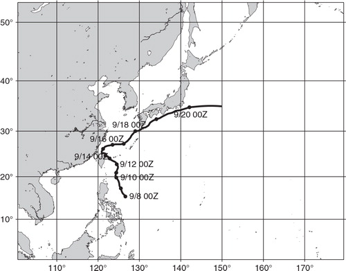
Miyoshi and Kunii (2012) performed experiments with the WRF-LETKF system and obtained a stable performance with realistic analyses compared with the National Centers for Environmental Prediction (NCEP) operational final analysis (FNL). This study employs the WRF-LETKF system with essentially the same configurations. The Advanced Research WRF (ARW) Version 3.2 is configured with a 60 km resolution and a domain spanning the Northwestern Pacific region (Fig. 1). The 40 vertical model levels extend up to 10 hPa at the model top. The experimental period starts on 6 August 2008, allowing about a one-month spin-up for Typhoon Sinlaku, a storm with its genesis in early September and that reached maturity around 10–12 September before making landfall in northern Taiwan on 13 September. Figure 1 shows the best track of Sinlaku, provided by the Regional Specialized Meteorological Center (RSMC) Tokyo – Typhoon Center (refer to Japan Meteorological Agency 2008 for the detailed description of Sinlaku). The ensemble size is fixed at 40 members, and the localisation parameters are chosen to be 400 km in the horizontal (~1460 km radius of influence), 0.4 in the ln p vertical coordinate (~1.46 radius of influence), and 3 h in time. The data assimilation cycle interval is 6 h.

Fig. 1.  Computational domain and the best track of Sinlaku.

Variance inflation (Anderson and Anderson, 1999) addresses the issue of variance underestimation, a typical problem in ensemble Kalman filter applications to NWP. The WRF-LETKF system can use two types of inflation methods: fixed multiplicative inflation and adaptive inflation (Anderson, 2007, 2009; Li et al., 2009; Miyoshi, 2011). Daley (1992) and Desroziers et al. (2005) derived the innovation statistics, which compare the forecast-minus-observation departures D (i.e. innovations) with forecast ensemble spread P and observation errors R: intuitively, D=P+R. This mathematical description is not rigorous or precise but is good for intuitive illustration – refer to Daley (1992) and Desroziers et al. (2005) for precise descriptions. Since the ensemble Kalman filter generally tends to underestimate the forecast ensemble spread P, usually D>P+R. To correct the mismatch, P is inflated by a factor of a to satisfy ideally D=aP+R. The fixed multiplicative inflation method uses a tuned constant inflation factor a. Alternatively, the adaptive inflation method estimates a adaptively using the innovation statistics at each analysis step at each grid point. To reduce the sampling noise at each step, the estimate a is temporally smoothed, so that the adaptive inflation factor adjusts slowly in time. In general, the underestimation of the ensemble spread P is very sensitive to the observing density. When the observations are dense (i.e. many observations in a given area), the ensemble spread is reduced excessively, that is, P becomes too small. Therefore, adaptive inflation will strongly depend on the observing density. The current adaptive inflation method of Miyoshi (2011), implemented in the present WRF-LETKF system, assumes temporal homogeneity of observing networks. Since Miyoshi and Kunii (2012) found that the adaptive inflation method generally outperformed the fixed multiplicative inflation method with this WRF-LETKF system, this study employs adaptive inflation.

Two experiments are performed: one with the NCEP PREPBUFR observation dataset (Keyser, 2010) and the other with additional AIRS retrievals. We call the experiment without AIRS data ‘CTRL’, and the one with AIRS data ‘AIRS’. Both CTRL and AIRS experiments use the same conventional observations from the NCEP PREPBUFR data downloaded from the University Corporation for Atmospheric Research (UCAR) online data server. The NCEP PREPBUFR data include upper-air soundings from radiosondes and dropsondes (ADPUPA), surface stations (ADPSFC), ships and buoys (SFCSHP), aircrafts (AIRCFT), and various types of remote sensing of winds (PROFLR, VADWND, SATWND, SPSSMI, QKSWND). The six-character codes of the observation types are defined in the PREPBUFR Table 1.a (Keyser, 2010). Only the AIRS experiment uses the AIRS Version 5 retrieval data downloaded from the NASA webpage (http://disc.sci.gsfc.nasa.gov/AIRS/data-holdings/). Among the various AIRS retrieval products, the AIRS Level-2 retrieval product based on AIRS and AMSU – AIRX2RET – is used in this study. AMSU is on the same spacecraft and collocated with AIRS and is included in the derivation of the retrieval data. The retrieval data are available over both land and ocean; Susskind et al. (2011) show that the retrieval data are generally less accurate over land. Readers interested in further details on the AIRS Version 5 retrieval data are referred to Susskind et al. (2011). This dataset includes 28 vertical levels, a subset of the more complete AIRX2SUP product that has 100 levels and which is what Reale et al. (2009) used. The retrieval product contains ‘best’ and ‘good’ quality flags; only the AIRS data with the ‘best’ quality are used in this study. The AIRS data are assimilated in the LETKF system exactly in the same manner as conventional observations, since each retrieved profile datum has its own specific location (longitude, latitude, and pressure level), observed value, and observation error standard deviation, and these are exactly what the LETKF system requires for conventional observations.

All quality-controlled AIRS retrieval data were initially assimilated as additional profile observations. This naive assimilation of AIRS retrievals was not successful mainly due to the high spatial density of AIRS data (about a 45 km resolution at nadir) relative to the model resolution (60 km) and probably because of significant observation error correlations between nearby profiles. The additional AIRS data clearly degraded the analyses and forecasts, although the data assimilation cycle performed stably. Therefore, a simple thinning algorithm is applied, so that one out of nine profiles is regularly selected for data assimilation. The horizontal thinning helps reduce the data density to be equivalent to a 135 km resolution, slightly more than twice the 60 km model resolution, and this probably also helps reduce the effect of the horizontal observation error correlations. The average number of AIRS data is greatly reduced from 140000 to be about 15000 per 6 h in the Northwestern Pacific domain and is comparable to the number of conventional observations (~22000 per 6 h).

However, assimilating the thinned AIRS data did not improve the analysis, or even worse, degraded the analysis significantly. A problematic behaviour was found in the time series of the analysis ensemble spread, which showed unrealistically large diurnal variations. This turned out to be tied to the large difference of the number of observations assimilated at 0000, 0600, 1200, and 1800 UTC. More specifically, the average number of AIRS data assimilated in the Northwestern Pacific domain was about 5000 per 6 h at 0000 and 1200 UTC, versus about 26000 per 6 h at 0600 and 1800 UTC (with these numbers obtained after applying the one-out-of-nine thinning). As previously mentioned, the different number of observations suggests different inflation factors at each time of day, but the adaptive inflation method of Miyoshi (2011) assumes temporally homogeneous observing networks and allows only slow adjustments in time.

This temporal inhomogeneity of AIRS coverage motivates and requires enhancing the adaptive inflation method. Kang et al. (personal communication) had a similar problem with their observing systems simulation experiments (OSSE) with simulated satellite data, and they found that ‘leap-frogging’ the adaptive inflation estimates, namely, defining separate inflation fields every 12 h, solved the problem of the large diurnal variations of ensemble spread and improved the analysis accuracy significantly. In this study, since the observing locations are unique to each time of the day, four different adaptive inflation fields are defined, corresponding to each assimilation time of 0000, 0600, 1200 and 1800 UTC. After applying this enhancement of adaptive inflation technique, the results started to show improvement due to the addition of AIRS data.

3. General verification results

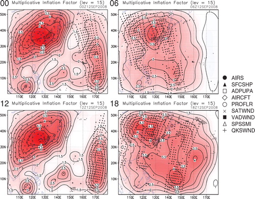
The observing locations per 6-h period and the corresponding adaptive inflation fields are shown in Fig. 2. Although Fig. 2 shows a single date (12 September), other dates show very similar patterns because the adaptive inflation fields vary slowly in time and because both conventional and AIRS observation locations are very similar on other dates. At 0000 and 1200 UTC, the AIRS observations are located only near the eastern boundary, where corresponding inflation values are as large as 3.5 (i.e. 250% covariance inflation). By contrast, significantly lower inflation is found in the eastern area at 0600 and 1800 UTC. At all four times, the largest inflation values appear in the northwestern quadrant near the Korean peninsula. Particularly larger inflation values of over 5.0 (400%) appear at 0000 and 1200 UTC, when radiosonde observations (RAOB) are available. Although only a few RAOB are available at 0600 and 1800 UTC, AIRS data have good coverage over land, making the inflation values nearly as large as those at 0000 and 1200 UTC.

Fig. 2.  Adaptive inflation fields (contours enhanced by shading) and assimilated observations (marked as described in the legend) at the 15th model level (~500 hPa) at 0000 (top left), 0600 (top right), 1200 (bottom left), 1800 (bottom right) UTC on 12 September 2008. The legend shows the observing types with six-character codes as defined in PREPBUFR Table 1.a (Keyser, 2010), except for the closed circles showing AIRS data.

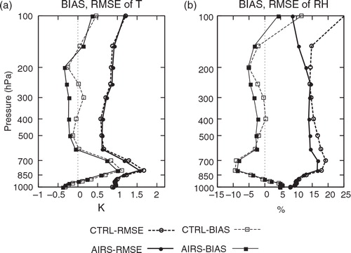
Since AIRS data add a significant number of observations of temperature and humidity profiles, we first investigate the analysis differences due to the inclusion of AIRS data. Figure 3 shows mean differences and RMS differences of the analyses of the CTRL and AIRS experiments relative to the NCEP FNL. The NCEP FNL is interpolated to the same 60 km grid of the WRF-LETKF system prior to taking the differences. The temperature analyses show cold biases due to AIRS data by about 0.5 K around 300 hPa, although the RMS fit to NCEP FNL shows no significant change due to AIRS data (Fig. 3a). If we look at humidity analysis differences (Fig. 3b), the RMS fit to NCEP FNL is significantly better at almost all levels due to AIRS data. This is not surprising since NCEP FNL assimilates AIRS radiances, and because AIRS data are the significant source of humidity observations in addition to RAOB. Fig. 3b also shows that AIRS data bring generally dry biases, particularly at 400, 300, 250, and 100 hPa levels. Although the AIRS data have different geographical distributions at 0000, 0600, 1200, and 1800 UTC, the horizontal patterns of the analysis differences cannot be distinguished between different analysis times, probably because the forecast-assimilation cycle results in smooth transitions in time.

Fig. 3.  Mean differences (squares) and RMS differences (circles) of (a) temperature analyses (K) and (b) relative humidity analyses (%) for CTRL (dashed) and AIRS (solid) experiments relative to NCEP FNL, averaged over 27 days from 1 to 27 September 2008. Squares and circles indicate mean errors and RMSE, respectively.

In order to assess the impact of AIRS data on forecasts, 72 h forecasts are verified relative to RAOB and NCEP FNL. The NCEP FNL is interpolated to the same 60 km grid of the WRF-LETKF system prior to verification. Here, deterministic 72 h forecasts are initiated from the most probable ensemble-mean analyses. The lateral boundary conditions for the 72 h forecasts are provided by the NCEP Global Forecasting System (GFS) forecasts in all experiments. An advantage of using NCEP FNL as a reference is its spatial homogeneity, whereas RAOB are mostly deployed from stations over land. In addition, NCEP FNL is independent of the WRF-LETKF cycle, whereas RAOB are assimilated in the WRF-LETKF cycle. The root mean square errors (RMSE) and mean errors are computed for 27 days from 1 to 27 September, which is comparable to the typical verification period of operational developments of regional NWP systems.

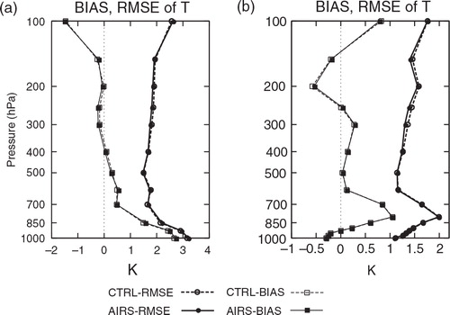
Figure 4 shows 72 h temperature forecast verifications, indicating slight but consistent improvement due to AIRS data in the middle to upper troposphere. In the lower troposphere, we find very little impact due to AIRS data.

Fig. 4.  72 h forecast verifications relative to (a) radiosonde observations and (b) NCEP FNL for temperature (K) for CTRL (dashed) and AIRS (solid) experiments, averaged over 27 days from 1 to 27 September 2008. Squares and circles indicate mean errors and RMSE, respectively.

Similar vertical profile figures as Fig. 4 are obtained for other variables and other forecast lead times. In order to look at many forecast times in a single figure, relative improvement is plotted by colour shading, so that a panel of Fig. 4 is now a single column of coloured circles as indicated by green boxes in Figs. 5 and 6. Here, the relative improvement was defined as follows:

Fig. 5.  Relative improvement (%) of RMSE due to AIRS data for (a) zonal wind, (b) meridional wind, (c) temperature, and (d) specific humidity. The RMSEs are relative to radiosonde observations. The positive values (red) correspond to improvement due to AIRS data. The green box corresponds to Fig. 4 (a). The number of observations used for the verifications at each level is about 600, except for temperature and humidity at 1000 hPa which have about 300 observations.

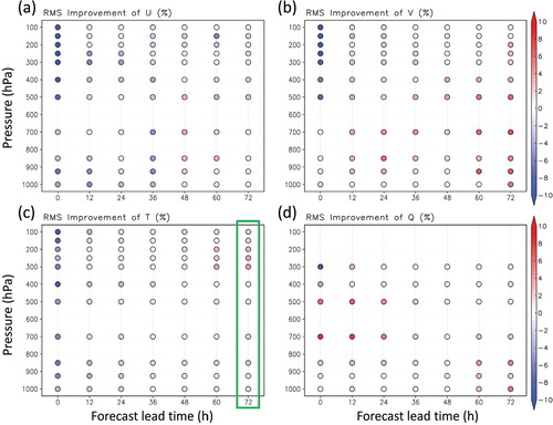
Fig. 6.  Similar to Fig. 5, but the RMSEs are relative to NCEP FNL, and (d) shows relative humidity instead of specific humidity. The green box corresponds to Fig. 4 (b).

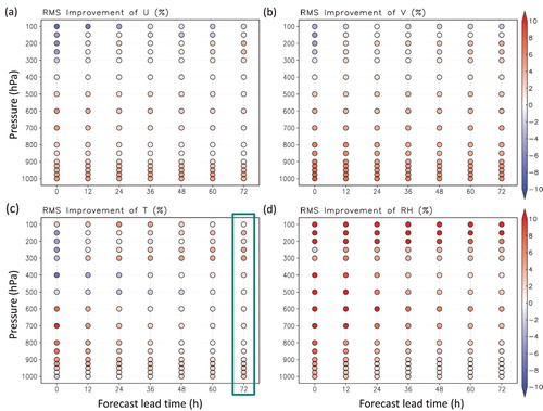
Figures 5 and 6 show the verifications relative to RAOB and NCEP FNL, respectively. The number of RAOBs used for the verifications at each level is about 600, except for temperature and humidity at 1000 hPa which have about 300 observations. When the surface pressure at the station is below 1000 hPa, no temperature or humidity observations are available for verification. At the analysis time (0 h forecast lead), the verifications relative to RAOB show mostly negative impact due to AIRS data (Fig. 5). This agrees with our expectations, since RAOB data are already assimilated in CTRL, and additional AIRS data would likely make the analysis fields closer to the AIRS data, and therefore, away from RAOB. Consequently, if we verify the analysis fields relative to RAOB, the additional AIRS data would result in larger RMSE. As forecast time progresses, we find generally more positive impacts due to AIRS data. Humidity verifications show positive impact from the beginning and will be discussed later.

The general tendency of more positive impacts of AIRS data in longer-lead forecasts is also apparent in the verifications relative to NCEP FNL (Fig. 6). Here, the lower troposphere shows general improvement due to AIRS at the analysis time (0 h forecast lead). Since NCEP FNL assimilates AIRS radiances, adding AIRS data may make the analyses closer to NCEP FNL. The advantage of adding AIRS data appears much clearer when verified relative to NCEP FNL than to RAOB, probably because of the contribution from the large area over the ocean. Wind fields are not observed by AIRS, but show significant improvements in Fig. 6. This is generally true for the verification relative to RAOB with respect to the meridional wind (Fig. 5b), but this is not clear for the zonal wind (Fig. 5a).

The humidity forecasts show general improvements both in Figs. 5 (d) and 6 (d). This is encouraging since AIRS data are a significant additional source of humidity observations, whereas in the CTRL experiment RAOB are almost the only source of humidity observations. The fact that even at the analysis time the humidity fields become closer to RAOB implies that the humidity fields in the forecast-analysis cycle would be generally improved. Namely, without AIRS data, the humidity fields may not be constrained well due to limited humidity observations, so that the additional AIRS data may constrain the humidity analysis better and result in a better fit to RAOB data. In fact, humidity verifications show consistent improvements at almost all forecast lead times and relative to both RAOB and NCEP FNL, with only a small number of exceptions.

4. AIRS impact on tropical cyclone forecasts

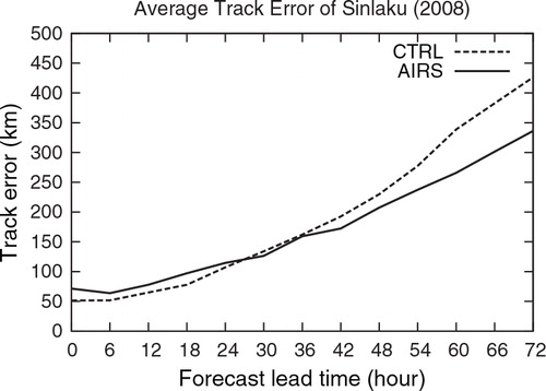
The general improvements in longer-lead forecasts shown in the previous section are more evident in tropical cyclone forecasts. This is demonstrated by Fig. 7, in which a single case of Sinlaku's track forecasts shows much improvement in longer-lead forecasts when using analyses that have assimilated AIRS data. It is difficult to find improvement in forecasts shorter than 36 h, but after that, the discrepancy of the forecast tracks becomes more and more apparent. Although Fig. 7 shows only a single case, the results are very similar on other dates. In fact, on average over 28 initial times during a week from September 8 to 14, we find essentially the same result (Fig. 8). Although during the initial 36-h forecasts the advantage of adding AIRS data is not significant, it becomes more apparent in longer-lead forecasts. Note that the model's grid spacing is 60 km, so that the average track error is less than the grid spacing up to about 12 h forecasts. The improvement of the average track error due to the addition of AIRS data reaches nearly 100 km in 72 h forecasts.

Fig. 7.  72 h forecast tracks of Sinlaku, initialised at 0600 UTC 12 September 2008 for the CTRL (blue) and AIRS (red) experiments. The black curve shows observed best track in the same period. Closed and open circles show the central position every 6 h.

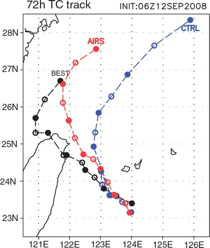
Fig. 8.  72 h forecast track errors (km) of Sinlaku of the CTRL (dashed) and AIRS (solid) experiments, averaged over 28 samples from 8 to 14 September 2008.

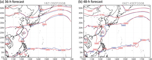
Sinlaku's track forecasts shown in Fig. 7 would likely be driven by the large-scale flow of the northwestern boundary of the subtropical Pacific high. We find the corresponding large-scale features in 500 hPa geopotential height fields (Fig. 9). Up to the 36 h forecast, little difference is found between CTRL and AIRS. However, for the 48 h forecast, we find a noticeable difference in the northwestern edge of the Pacific high; the 5880 m contour extends to the west in AIRS, corresponding to the delayed recurvature of Sinlaku. This suggests that AIRS data would have improved large scales, which have slower response, perhaps explaining the results that the AIRS impact was generally more apparent in longer-lead forecasts. We note that the lateral boundary conditions are identical in both AIRS and CTRL experiments, so that the larger scales beyond what is represented within the model domain must have come from the NCEP GFS boundary conditions.

Fig. 9.  500 hPa geopotential height forecasts (m) at (a) 36 h and (b) 48 h forecast lead times initialised at 0600 UTC 12 September 2008 for the CTRL (blue) and AIRS (red) experiments.

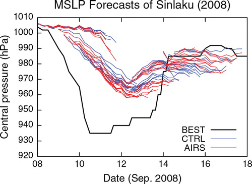
Sinlaku's intensity forecasts are also substantially improved by the assimilation of AIRS data. Apparently, the 60 km resolution is too coarse to resolve Sinlaku's inner structure. Kunii et al. (2012) found that inner-core observations were not useful at this resolution using the WRF-LETKF system; this generally agrees with previous studies (e.g. Aberson, 2008; Weissmann, et al. 2011). Yet, Fig. 10 shows significant advantages of using AIRS data in Sinlaku's central pressure forecasts. Although the deep structure of Sinlaku are not well captured, the forecasts with AIRS data show better agreement with the best track data, particularly the stronger stage before the landfall in Taiwan, and the weakened stage after the landfall, around 11 to 15 September.

Fig. 10.  72 h minimum central pressure forecasts of Sinlaku of the CTRL (blue) and AIRS (red) experiments, each line corresponding to different initial times (total 28 initial times from 8 to 14 September). The observed best track is shown by the black line.

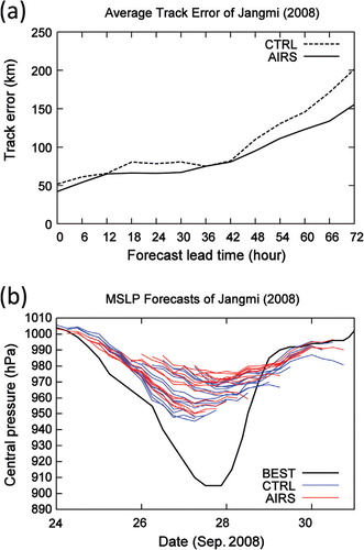
For investigating the case-dependency of the above results, similar verifications are examined for the case of Typhoon Jangmi. Jangmi formed about 1000 km east of the Philippines on 24 September 2008, developed consistently at a relatively rapid rate for two days to reach its minimum central pressure of 905 hPa on 27 September, and made its landfall in Taiwan on 28 September. Figure 11 shows the comparison of the track and intensity forecasts between AIRS and CTRL. Similarly to Sinlaku, AIRS data show a positive impact on the track forecasts, particularly for longer-lead forecasts after 48 h (Fig. 11a). The 72 h track forecasts are improved by about 50 km on average, almost one grid spacing. However, the improvement of intensity forecast is unclear (Fig. 11b). In the early stage of the development up to 25 September, AIRS shows clear improvement of intensity forecasts. However, after 26 September, when Jangmi develops its intensity deeper than about 950 hPa, AIRS shows consistently weaker typhoon forecasts than the CTRL. Further discussion about intensity forecasts requires higher-resolution experiments, which are to be a subject of future research.

Fig. 11.  Similar to Figs. 8 and 10, but for Typhoon Jangmi (2008). (a) 72 h forecast track errors (km) averaged over 16 samples from 24 to 27 September, and (b) 72 h minimum central pressure forecasts, each line corresponding to different initial times (total 16 initial times from 24 to 27 September).

5. Summary and discussion

This study showed that assimilation of both temperature and humidity profile data from the AIRS Version 5 retrieval products using the WRF-LETKF system improved regional NWP, particularly for humidity and in longer-lead forecasts. Also, track forecasts of Typhoons Sinlaku and Jangmi were substantially improved due to the inclusion of AIRS data. In order to obtain these improvements, additional developments of horizontal data thinning and enhancing adaptive inflation played an essential role. The improvements obtained in this study generally agree with previous studies that showed improvement of NWP skills due to AIRS data (Le Marshall et al., 2006; McNally et al., 2006; Wu et al., 2006; Reale et al., 2008, 2009), and suggest the usefulness of AIRS data in regional NWP.

Although this study employed a relatively low 60 km resolution, the results showed a potential for improving the intensity forecasts of Tropical Cyclones (TC). Typhoon Sinlaku had the peak intensity of 935 hPa, and the addition of AIRS data resulted in consistently improved intensity forecasts, although, as expected, the 60 km resolution yielded a systematically shallower typhoon. In the case of Typhoon Jangmi, Jangmi had the even stronger peak intensity of 905 hPa, and the additional AIRS data did not improve intensity forecasts after Jangmi became deeper than about 950 hPa. More cases are necessary to draw general conclusions on what impact AIRS data may have on TC intensity forecasts. Also, higher-resolution experiments are essential to resolve mesoscale processes within the TC inner structure, which would have an important role in changing TC intensity. Such further investigations remain the subject of future research.

Another limitation of this study is the absence of other satellite sounder and imager data. This study focused on the impact of AIRS retrieval data on top of conventional observations. Operational NWP usually assimilates AMSU and other sounder and imager instruments of different spacecraft, so the impact of AIRS in the presence of these other satellite data may be of interest to the operational community. Adding more satellite data is an important future extension of this study.

In the course of the developments in this study, three major issues appeared and remain to be fully explored: intelligent data thinning, treatment of observation error correlations, and fundamental treatment of temporally inhomogeneous observing networks. This study employed a simple, regular selection of one out of nine observations. This can be improved by either using adaptive observation strategies to select the most helpful locations (e.g. Ochotta et al., 2005), or a super-observation strategy which synthesises a super-observation by combining multiple nearby observations (e.g. Lorenc, 1981). These intelligent thinning methods are widely applicable to other types of dense observations, and a number of previous studies exist. Also, this study assumed uncorrelated observation errors. As mentioned in introduction, proper inclusion of observation error correlations in data assimilation is an important issue that can lead to more wisely using retrieval information. As for treating temporally inhomogeneous observing networks, this study employed an ad-hoc approach of “leap-frogging” of adaptive inflation, following the success of Kang et al. (personal communication). Fundamental theoretical development of relaxing the assumption of temporally-fixed observing networks in adaptive inflation is an important subject of future research.

6. Acknowledgements

The authors thank Steven Greybush and other members of the UMD Weather-Chaos Group, Oreste Reale of NASA/GSFC, and Sharan Majumdar of University of Miami for fruitful discussions. The NCEP PREPBUFR observation data were obtained from the UCAR data server, while several missing files were kindly provided by Daryl Kleist of NCEP. This study was supported by the Office of Naval Research (ONR) grant N000141010149 under the National Oceanographic Partnership Program (NOPP).

References

- Aberson S. D. Targeted observations to improve operational tropical cyclone track forecast guidance. Mon. Wea. Rev. 2003; 131: 1613–1628. 10.3402/tellusa.v64i0.18408.
- Anderson J. L. An adaptive covariance inflation error correction algorithm for ensemble filters. Tellus. 2007; 59A: 210–224.
- Anderson J. L. Spatially and temporally varying adaptive covariance inflation for ensemble filters. Tellus. 2009; 61A: 72–83.
- Anderson J. L. Anderson S. L. A Monte Carlo implementation of the nonlinear filtering problem to produce ensemble assimilations and forecasts. Mon. Wea. Rev. 1999; 127: 2741–2758.
- Aumann, H. H, Chahine, M. T, Cautier, C, Goldberg, M. D, Kalnay, E and co-authors. 2003. AIRS on the Aqua mission: Design, science objectives, data products, and processing systems. IEEE Trans. Geosci. Remote Sens. 41, 253–264. 10.3402/tellusa.v64i0.18408.
- Daley R. Estimating model-error covariances for application to atmospheric data assimilation. Mon. Wea. Rev. 1992; 120: 1735–1746.
- Desroziers G. Berre L. Chapnik B. Poli P. Diagnosis of observation, background and analysis-error statistics in observation space. Quart. J. Roy. Meteor. Soc. 2005; 131: 3385–3396. 10.3402/tellusa.v64i0.18408.
- Fourrié N. Thépaut J.-N. Evaluation of the AIRS near-real-time channel selection for application to numerical weather prediction. Quart. J. Roy. Meteor. Soc. 2003; 129: 2425–2439. 10.3402/tellusa.v64i0.18408.
- Hunt B. R. Kostelich E. J. Szunyogh I. Efficient data assimilation for spatiotemporal chaos: a local ensemble transform Kalman filter. Physica. D. 2007; 230: 112–126. 10.3402/tellusa.v64i0.18408.
- Japan Meteorological Agency. 2008. Annual Report on the Activities of the RSMC Tokyo – Typhoon Center (2008). 80. Online at: http://www.jma.go.jp/jma/jma-eng/jma-center/rsmc-hp-pub-eg/AnnualReport/2008/Text/Text2008.pdf.
- Kang, J.-S, Kalnay, E, Miyoshi, T, Liu, J and Fung, I. (personal communication) Estimation of surface carbon fluxes with an advanced data assimilation methodology. In preparation.
- Keyser, D. 2010. PREPBUFR Processing at NCEP. Online at: http://www.emc.ncep.noaa.gov/mmb/data_processing/prepbufr.doc/document.htm.
- Kunii, M, Miyoshi, T and Kalnay, E. 2012. Estimating impact of real observations in regional numerical weather prediction using an ensemble Kalman filter. Mon. Wea. Rev. 140, 1975–1987. DOI:10.3402/tellusa.v64i0.18408.
- Le Marshall, J, Jung, J, Derber, J, Chahine, M, Treadon, R and co-authors. 2006. Improving global analysis and forecasting with AIRS. Bull. Amer. Meteor. Soc. 87, 891–894. 10.3402/tellusa.v64i0.18408.
- Li H. Kalnay E. Miyoshi T. Simultaneous estimation of covariance inflation and observation errors within an ensemble Kalman filter. Quart. J. Roy. Meteor. Soc. 2009; 135: 523–533. 10.3402/tellusa.v64i0.18408.
- Lorenc A. C. A global three dimensional multivariate statistical interpolation scheme. Mon. Wea. Rev. 1981; 109: 701–721.
- McNally, A. P, Watts, P. D, Smith, J. A, Engelen, R, Kelly, G. A and co-authors. 2006. The assimilation of AIRS radiance data at ECMWF. Quart. J. Roy. Meteor. Soc. 132, 935–957. 10.3402/tellusa.v64i0.18408.
- Miyoshi, T. 2011. The Gaussian approach to adaptive covariance inflation and its implementation with the local ensemble transform Kalman filter. Mon. Wea. Rev. 139, 1519–1535. DOI:10.3402/tellusa.v64i0.18408.
- Miyoshi, T and Kunii, M. 2012. The local ensemble transform Kalman filter with the Weather Research and Forecasting model: experiments with real observations. Pure and Appl. Geophys. 169, 321–333. DOI:10.3402/tellusa.v64i0.18408.
- Miyoshi, T, Kalnay, E and Li, H. 2012. Estimating and including observation error correlations in data assimilation. Inverse Problems in Science and Engineering. OI:10.3402/tellusa.v64i0.18408.
- Ochotta, T, Gebhardt, C, Saupe, D and Wergen, W. 2005. Adaptive thinning of atmospheric observations in data assimilation with vector quantisation and filtering methods. Quart. J. Roy. Meteor. Soc. 131, 3427–3437. DOI:10.3402/tellusa.v64i0.18408.
- Reale, O, Susskind, J, Rosenberg, R, Brin E, Liu E and co-authors. 2008. Improving forecast skill by assimilation of quality-controlled AIRS temperature retrievals under partially cloudy conditions. 35, L08809.10.3402/tellusa.v64i0.18408.
- Reale, O, Lau, W. K, Susskind, J, Brin E, Liu E and co-authors. 2009. AIRS impact on the analysis and forecast track of tropical cyclone Nargis in a global data assimilation and forecast system. Geophys. Res. Lett. 36, L06812.10.3402/tellusa.v64i0.18408.
- Rodgers, C. D. 2000. Inverse Methods for Atmospheric Sounding: Theory and Practice. World Scientific, Singapore. pp. 256.
- Skamarock, W. C, Klemp, J. B, Dudhia, J, Gill, D. O, Barker, D. M and co-authors. 2005. A Description of the Advanced Research WRF Version 2. NCAR Tech. Note TN-468+STR, 88. pp.
- Susskind, J. 2007. Improved atmospheric sounding and error estimates from analysis of AIRS/AMSU data. 6684, 66840M. DOI:10.3402/tellusa.v64i0.18408.
- Susskind, J. 2011. Improved temperature sounding and quality control methodology using AIRS/AMSU Data: The AIRS Science Team Version 5 retrieval algorithm. Proc. SPIE. 49, 883–907. DOI:10.3402/tellusa.v64i0.18408.
- Susskind J. Barnet C. Blaisdell J. M. Retrieval of atmospheric and surface parameters from AIRS/AMSU/HSB data in the presence of clouds. IEEE Trans. Geosci. Remote Sens. 2003; 41: 390–409. 10.3402/tellusa.v64i0.18408.
- Susskind, J, Barnet, C, Blaisdell, J, Iredell, L, Keita, F and co-authors. 2006. Accuracy of geophysical parameters derived from Atmospheric Infrared Sounder/Advanced Microwave Sounding Unit as a function of fractional cloud cover. IEEE Trans. Geosci. Remote Sens. 111. D09S017.10.3402/tellusa.v64i0.18408.
- Weissmann, M, Harnisch, F, Wu, C. C, Lin, P. H, Ohta, Y and co-authors. 2011. The influence of assimilating dropsonde data on typhoon track and mid-latitude forecasts. J. Geophys. Res. 139, 908–920. 10.3402/tellusa.v64i0.18408.
- Wu, L, Braun, S. A, Qu, J. J and Hao, X. 2006. Simulating the formation of Hurricane Isabel (2003) with AIRS data. Mon. Wea. Rev. 33, L04804.10.3402/tellusa.v64i0.18408.