A hybrid nudging-ensemble Kalman filter approach to data assimilation. Part I: application in the Lorenz system

ABSTRACT

A hybrid data assimilation approach combining nudging and the ensemble Kalman filter (EnKF) for dynamic analysis and numerical weather prediction is explored here using the non-linear Lorenz three-variable model system with the goal of a smooth, continuous and accurate data assimilation. The hybrid nudging-EnKF (HNEnKF) computes the hybrid nudging coefficients from the flow-dependent, time-varying error covariance matrix from the EnKF's ensemble forecasts. It extends the standard diagonal nudging terms to additional off-diagonal statistical correlation terms for greater inter-variable influence of the innovations in the model's predictive equations to assist in the data assimilation process. The HNEnKF promotes a better fit of an analysis to data compared to that achieved by either nudging or incremental analysis update (IAU). When model error is introduced, it produces similar or better root mean square errors compared to the EnKF while minimising the error spikes/discontinuities created by the intermittent EnKF. It provides a continuous data assimilation with better inter-variable consistency and improved temporal smoothness than that of the EnKF. Data assimilation experiments are also compared to the ensemble Kalman smoother (EnKS). The HNEnKF has similar or better temporal smoothness than that of the EnKS, and with much smaller central processing unit (CPU) time and data storage requirements.

• ensemble Kalman filter (EnKF)
• nudging
• hybrid data assimilation
• error spikes
• dynamic analysis
• Lorenz system

1. Introduction

Data assimilation combines the observations and the forecast by a numerical weather prediction model to produce an analysis. The analysis is considered as the best estimate of the current state of the atmosphere. Thus, an important objective of the data assimilation is to develop optimal methods to assimilate the observations to provide the best possible analysis and initialisation for the forecast model.

The ensemble Kalman filter (EnKF) is currently a popular data assimilation method. The EnKF was first proposed by Evensen (1994) in an oceanographic application and has subsequently been implemented in atmospheric applications (e.g. Houtekamer and Mitchell, 1998; Anderson, 2001; Whitaker and Hamill, 2002). The EnKF uses the statistical properties of an ensemble forecast to estimate the flow-dependent background error covariances. These flow-dependent background error covariances determine how an observation affects the model variables. Then, a new analysis ensemble with the statistics to minimise the analysis error is produced. By contrast, the three-dimensional variational method (3DVAR; Sasaki, 1970; Lorenc, 1986; Courtier et al., 1998), which assimilates observations sequentially and is computationally efficient, generally adopts a homogeneous and stationary background error covariance. The four-dimensional variational method (4DVAR; Lorenc, 1986; Thepaut et al., 1993), which finds the trajectory that best fits the past and present observations, generally requires a tangent linear model and adjoint model to estimate the actual flow-dependent error structure. Therefore, the EnKF is becoming increasingly popular compared to 3DVAR and 4DVAR methods, because it is able to efficiently compute the flow-dependent background error covariances from an ensemble forecast without requiring a tangent linear model and adjoint model (e.g. Houtekamer and Mitchell, 1998; Fujita et al., 2007).

To combine the advantages of EnKF and variational data assimilation methods, several hybrid data assimilation schemes have been studied. For example, a hybrid EnKF–3DVAR has been discussed by Hamill and Snyder (2000), in which the background error covariances are a linear combination of the stationary covariances used in 3DVAR and flow-dependent covariances computed from a short-range ensemble forecast. A hybrid ensemble transform Kalman filter (ETKF; Bishop et al., 2001)–3DVAR has been proposed by Wang et al. (2008a, b). The hybrid ETKF–3DVAR combines the ensemble covariances with the static covariances used in 3DVAR, incorporates these covariances during the variational minimisation by the extended control variable method and maintains the ensemble perturbations by the ETKF. An ensemble-based 4DVAR (En4DVAR), developed by Liu et al. (2008), uses an ensemble forecast to provide the flow-dependent background error covariances and performs 4DVAR optimisation without tangent linear and adjoint models.

However, the EnKF is an intermittent data assimilation approach, where observations are processed in small batches intermittently in time. The intermittent nature of the EnKF often causes discontinuities/error spikes around the observation times (e.g. Hunt et al., 2004; Fujita et al., 2007). Juckes and Lawrence (2009) reported similar ‘discontinuities’ in the forward and backward Kalman filter analyses. Duane et al. (2006) also found that the Kalman filter algorithm has some ‘desynchronisation bursts’ at times of regime transitions between the Lorenz and ‘reversed Lorenz’ phases. Thus, the EnKF can produce discontinuities between the forecast and the analysis estimates. These discontinuities can introduce a shock at the model restart stage and cause spurious high-frequency oscillations and possibly lead to data rejection (Bloom et al., 1996; Ourmieres et al., 2006). Also because of the discontinuities, the ability of the EnKF to provide a time-continuous and seamless analysis is not guaranteed.

A time-continuous, seamless meteorological field is preferred in many applications, especially for use in driving air-quality and atmospheric-chemistry models (e.g. Stauffer et al., 2000; Tanrikulu et al., 2000; Otte, 2008a, b). Improved meteorological conditions and seamless meteorological background fields can also improve the simulation of transport and dispersion (e.g. Deng et al., 2004; Deng and Stauffer, 2006). Thus, it is hypothesised here that if the EnKF could be applied gradually in time, a dynamic analysis where data assimilation is applied throughout a model integration period would be produced, and the intermittent discontinuities and error bursts would be reduced.

The discontinuous nature of the analysis increments of the EnKF is recognised and discussed by Bergemann and Reich (2010) using a Lorenz system. They proposed a ‘mollified’ EnKF, which is able to damp the spurious high-frequency adjustment processes caused by the discontinuous EnKF. They note that the term ‘mollification’ introduced by Friedrichs (1944) denotes families of smooth functions that approach the Dirac delta function as the width of the time window approaches zero. In the ‘mollified’ EnKF, each ensemble member assimilates the observations by the continuous EnKF with a mollified Dirac delta function at every time step within a time window.

A hybrid nudging-EnKF (HNEnKF) is proposed here with the same purpose as the mollified EnKF. The HNEnKF applies the EnKF gradually in time by directly combining the EnKF with nudging. Compared to the mollified EnKF that calculates the nudging coefficients from the background error covariance and observational cost function at every time step and updates each ensemble member gradually in time, the HNEnKF computes the EnKF gain matrix once at the observation time and uses this EnKF gain matrix over the nudging time window within the nudging coefficients for one control member only. Therefore, the HNEnKF proposed here is more computationally efficient and may be more practical than the mollified EnKF for more complex models.

Nudging, also known as Newtonian Relaxation, is a continuous data assimilation method that relaxes the model state towards the observations by adding artificial terms to the prognostic equations (Hoke and Anthes, 1976). The artificial terms are proportional to the difference between the observations and the model state. Nudging is designed to be applied at every time step, allowing the corrections to be relatively small and applied gradually within a time window around the observation times (Stauffer and Seaman, 1990, 1994). Nudging has been used in many data assimilation applications (e.g. Stauffer and Seaman, 1990, 1994; Stauffer et al., 1991; Seaman et al., 1995; Leidner et al., 2001; Otte et al., 2001; Deng et al., 2004; Deng and Stauffer, 2006; Schroeder et al., 2006; Dixon et al., 2009; Ballabrera-Poy et al., 2009). However, it is typically used with ad hoc nudging coefficients and spatial weighting functions based on experience and experimentation. Adjoint parameter-estimation approaches have also been investigated using simple models to determine the optimal coefficients (Zou et al., 1992; Stauffer and Bao, 1993). When ensemble forecasts are available, the ensemble and the EnKF may provide a more practical alternative for determining the nudging coefficients.

Similar to nudging, the incremental analysis update (IAU; Bloom et al., 1996; Ourmieres et al., 2006; Lee et al., 2006) and the ensemble Kalman smoother (EnKS; Cohn et al., 1994; Evensen and van Leeuwen, 2000) are also continuous data assimilation methods. The IAU method incorporates the analysis increments into the model integration in a gradual manner as a state-independent forcing term (Bloom et al., 1996). Comparatively, the nudging adds a state-dependent forcing term into the model integration, because the state variables used in the additional nudging terms vary with time. Therefore, IAU does not consider the changes to the difference between the observation and the model state (the innovation) during the model integration. Thus nudging rather than IAU is chosen here as a means of applying the EnKF gradually in time.

The EnKS uses the EnKF solution as the first guess for the analysis and applies future observations backwards in time using the ensemble covariances. As an extension of EnKF, the EnKS is a continuous data assimilation method, and it uses an ensemble forecast to compute both the spatial and temporal error covariances. Thus, we treat the EnKS (Evensen and van Leeuwen, 2000; Whitaker and Compo, 2002; Khare et al., 2008) as the ‘gold standard’ against which to measure the success of other data assimilation methods as a benchmark.

The goal of this current study is to demonstrate that one can combine the advantages of the EnKF approach to data assimilation with the temporal smoothness of the continuous nudging approach. The HNEnKF proposed here uses nudging-type terms to apply the EnKF gradually in time in order to minimise the insertion shocks. The HNEnKF also has the ability to provide both the direction and the coupling strength from the EnKF to the nudging approach. Therefore, it is hypothesised that this hybrid combination of data assimilation methods should perform better than either method applied separately. To investigate the hypothesis that a continuous and seamless analysis can be produced if the EnKF is applied gradually in time, the proof of concept of this HNEnKF is first undertaken here in Part I using the Lorenz three-variable system (Lorenz, 1963).

The Lorenz three-variable model has served as a test bed for examining the properties of various data assimilation methods when used in systems with strongly non-linear dynamics (e.g. Evensen and van Leeuwen, 2000; Yang et al., 2006; Chin et al., 2007; Auroux and Blum, 2008; Pu and Hacker, 2009). The data assimilation techniques force a slave simulation towards a master simulation that represents the truth. This is similar to the approach taken by Yang et al. (2006), who extended the nudging approach from a single constant direction to a dynamically evolving direction given by either the bred vector or the singular vector when coupling the slave to the master. The coupling strength (nudging coefficient) necessary to achieve synchronisation between the slave and master simulations was tested over a wide range of values (1–100), but without any consideration of the relative size of the nudging term to the physical terms in the model equations and the potential creation of insertion noise. In this present study, several different data assimilation approaches are applied to the slave system. In addition to measuring the resulting error, the smoothness of the slave system is also measured using a new metric.

The general methodology of this HNEnKF is discussed in Section 2. Section 3 describes the Lorenz three-variable model system and the application of the HNEnKF in this system. Section 4 introduces the evaluation plan and performance metrics, and the experimental design is discussed in Section 5. Section 6 presents and discusses the results. Conclusions are summarised in Section 7. The HNEnKF is further explored in a two-dimensional shallow-water model in Part II (Lei et al., 2012). The investigation of the HNEnKF in this two-part study will set the stage for the implementation of HNEnKF in the three-dimensional Weather Research and Forecasting (WRF) model: its results will be presented in another paper (accepted by Q. J. R. Meteorol. Soc.).

2. General methodology for the HNEnKF approach

The evolution of a dynamical system can be represented as:1

where x and f are the state vector and dynamics function of the system, respectively.

Given an observation y ^o, the analysis step of the EnKF consists of the following update (Evensen, 1994):2

where x ^f is the model forecast or background, x ^a is the analysis, H is the observation operator that transforms or interpolates the model forecast variable to the observation variable and location and K is the gain matrix of the EnKF. This gain matrix is defined as:3

where B is the covariance matrix of background errors and R is the covariance matrix of observation errors.

On the other hand, the basic form of a dynamical data assimilation system using traditional nudging can be written as:4

wherein the time derivative and model physics terms are as in eq. (1), but a new term is added to relax or nudge the model background towards the observations. In eq. (4), G is the nudging magnitude matrix and w is the nudging spatial-temporal weighting coefficient used to apply the innovation (observation minus the model background, y ^o – HX) in observation space and time to the model grid cell and time step. The product of G and w is defined here as the nudging coefficient matrix.

The traditional nudging data assimilation scheme uses a nudging coefficient matrix with non-zero diagonal elements and zero off-diagonal elements; thus, innovations from one variable do not directly affect the others in the current time step. The nudging term is also kept small compared to the physical term, f(x), so that the model dynamics still play a major role in the data assimilation. The nudging coefficient matrix is often specified by experience and experimentation (e.g. Stauffer and Seaman, 1994) to emulate the error covariance, the correlation in the error at the observation location with that in a spatial region/temporal window about the observation site/observation time.

Compared to the intermittent data assimilation scheme EnKF, the HNEnKF method introduced here combines the continuous data assimilation of nudging with the flow-dependent weighting of EnKF to achieve a flow-dependent, continuous and gradual data assimilation. The HNEnKF builds the gain matrix of the EnKF into the nudging magnitude matrix (Kalata, 1984; Painter et al., 1990), which provides flow-dependent/time-dependent nudging coefficients to the traditional nudging. In other words, the HNEnKF achieves the analysis of the EnKF gradually by combining it with nudging.

For the HNEnKF data assimilation scheme presented here, the nudging magnitude matrix G in eq. (4) is a function of the EnKF gain matrix. Since the nudging assimilates the observed state gradually via the model tendency equations, the EnKF gain matrix should be modified in order to be applied to the nudging magnitude matrix. Thus, the nudging magnitude matrix in the HNEnKF method takes the form:5

where t _w has the units of inverse time and must be made a function of the nudging weighting coefficient w, in order to spread the magnitude of the EnKF gain matrix to every nudging time step. Thus, the definition of t _w can vary as long as its unit remains inverse time and it is a function of the nudging weighting coefficient.

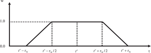
Specifically, in the Lorenz three-variable model system, the nudging weighting coefficient w only varies in time because the model state has no spatial extent. The Stauffer and Seaman (1990) trapezoidal function, as shown in Fig. 1, is used for this temporal weighting w. In Fig. 1, t is the model time, t ^o is the observation time and τ _N is the half-period of the nudging time window. Given τ _N, w and the time step Δt, the function t _w in eq. (5) is defined as the inverse of the sum of the nudging temporal weighting coefficient in the half-period of the nudging time window:6

Fig. 1.  The temporal weighting function w of nudging, where t is the model time, t ^o is the observation time and τ _N is the half-period of nudging time window (after Stauffer and Seaman, 1990).

Thus, the nudging strength summed from the start of nudging to the observation time equals the EnKF gain. After the observation time, the nudging term, the product of the nudging weights and the innovation, becomes smaller in magnitude as the nudging temporal weighting coefficient decreases, and the combined effects of the model's physical forcing and the data assimilation can further reduce the innovation. Linear model tests confirm that the nudging term decreases after the observation time, and the total increment during the nudging time window of the HNEnKF is less than 10% larger than that of the EnKF (not shown).

Compared to traditional nudging, this HNEnKF takes advantage of ensemble forecasts to obtain a flow-dependent/time-dependent background error covariance matrix that can be used to compute a flow-dependent/time-varying nudging coefficient matrix. The HNEnKF approach can also be used to extend the nudging magnitude matrix to include the inter-variable influence of innovations via non-zero off-diagonal elements. This additional coupling between the observations and the multivariate state may lead to more accurate adjustment of the background to observations than the traditional nudging approach. Therefore, the HNEnKF is an advancement beyond the current capabilities of traditional nudging.

3. Model description and methodology for the Lorenz system

As a test bed for data assimilation, the non-linear Lorenz three-variable model system offers the advantages of computational simplicity and strong non-linear interactions among variables (Lorenz, 1963). The model consists of three coupled and non-linear ordinary differential equations:7

where the parameters are set to the standard values that produce a chaotic regime: σ=10, r=28, b=8/3 (Lorenz, 1963).

For the HNEnKF approach, the system [eq. (7)] becomes:8

where each G is an element in the nudging magnitude matrix G in eq. (4). In the traditional nudging approach, only the diagonal elements of the nudging magnitude matrix are non-zero. In contrast, for the HNEnKF, all elements of this matrix can be non-zero. Compared to the adaptive nudging in Yang et al. (2006), here the EnKF gain matrix is used to provide both nudging direction and nudging strength.

The general procedures of the HNEnKF are shown in Fig. 2. The ensemble state contains ensemble members that are used to calculate the hybrid nudging magnitude matrix. The nudging state is a single member that assimilates observations by nudging with the hybrid nudging coefficients. The method for creating the initial conditions of the nudging state and ensemble state is described in Section 5. Both the ensemble state and nudging state are integrated forward until an observation is available. The observations are denoted by the arrows. When an observation is available, the EnKF gain matrix K is first computed from the ensemble forecast of the ensemble state, and then the hybrid nudging magnitude matrix G(K, t _w) is provided to the nudging state. The nudging state then assimilates the observation via eq. (8) using these hybrid nudging coefficients. The trapezoid around the observation in the nudging state defines the nudging time window. Meanwhile the ensemble state assimilates the observation by the EnKF. After both the nudging state and ensemble state finish assimilating the observation at the observation time, the ensemble members are shifted by the difference between the ensemble mean and the nudging state. This results in a new ensemble state centred on the nudging state. Thus, the ensemble spread of the ensemble state has been updated by the EnKF, and the ensemble mean of the ensemble state is defined to be the same as that of the nudging state at the observation time. Finally, both the ensemble state and the nudging state are integrated forward simultaneously. This procedure cycles when the next observation becomes available.

Fig. 2.  Schematic showing the procedures of the HNEnKF approach. The trapezoid around the observation denotes the temporal nudging weighting function over the nudging time window.

4. Evaluation plan and performance metrics

We are not aware of any previous studies that provide a metric to quantitatively measure the discontinuities/error spikes resulting from the intermittent data assimilation method EnKF. It is suggested here that the average root mean square (RMS) error that is widely used in the data assimilation literature should not be the only measure of success because it may not reflect the model's retention of data following the assimilation. Thus, a new metric is proposed here to quantitatively measure the error spikes/discontinuities following data assimilation.

This metric, defined as the discontinuity parameter (DP), is the average absolute value of the RMS error difference over the observation times, where the RMS error difference is the difference between the RMS error at one time step before the observation time and that at the observation time:9

where the RMSE denotes the RMS error, the subscript i represents the time step when an observation is available and M is the total number of the observation times.

As shown by eq. (9), the larger values of DP represent the larger error spikes/discontinuities and stronger imbalances caused by data assimilation. The DP of the EnKF can be large if the EnKF makes strong and instantaneous changes to the model state. The DP of the HNEnKF, on the other hand, can be much smaller than that of the EnKF if the HNEnKF effectively applies the EnKF gradually in time during the nudging time window as designed. Therefore, both the RMS error and DP will be used to evaluate the data assimilation methods, since the RMS error measures the success of a data assimilation method to fit the observations, and the DP measures the error spikes/discontinuities caused by a data assimilation method.

5. Experimental design

The truth state is obtained by integrating the equations in eq. (7) from a true initial value (1.508870, −1.531271 and 25.46091). Observation errors chosen randomly from a Gaussian distribution with mean zero and variance 1.0 are added to the true state (the master) to obtain the simulated observations. The signal to noise ratios1 of variables x, y and z are 62.98, 81.38 and 72.75, respectively. The observations of all three variables are available. The observation frequency for data assimilation is one per 25 time steps by default, and then it is varied to one per 10 and one per 50 time steps as sensitivity experiments. Similarly, adding a random error to the true initial value produces a simulated initial value to emulate the real atmosphere, because the true initial value is unknown in the real atmosphere. This simulated initial value is used as the initial condition of the nudging state as shown in Fig. 2. By adding random errors from a Gaussian distribution with mean zero and variance 1.0 to the simulated initial value, the initial values for an ensemble are derived. Similarly, these initial values are used as the initial conditions of the ensemble state as shown in Fig. 2. The ensemble size is set to 100, because the performance of the EnKF saturates quickly as the ensemble size increases in the Lorenz three-variable model system (Chin et al., 2007), and 100 members is the maximum ensemble size used in the sensitivity study of EnKF to the ensemble size in Pu and Hacker (2009). Experiments are first performed using a perfect model assumption. Then, a stochastic process following Evensen (1997) is added to the model equations to simulate the model error. The model error covariance is defined to be diagonal with variances (2.00, 12.13 and 12.31) for the three equations in eq. (7) (Evensen, 1997; Evensen and van Leeuwen, 2000). Both the perfect and imperfect models are integrated in time using a fourth-order Runge-Kutta time difference scheme with a time step Δt=0.01. We found that using a smaller time step of 0.001 does not change the results.

To eliminate the effects of start-up transients, the slave Lorenz system from the simulated initial value and the ensemble are integrated for 1000 time steps before beginning to assimilate the observations as in Yang et al. (2006). During the data assimilation phase, the EnKF, EnKS, traditional nudging, IAU and HNEnKF are each integrated for 3500 time steps. The first 500 time steps of the data assimilation cycle are discarded similar to Yang et al. (2006), and then the following 3000 time steps with data assimilation are used for analysis.

The results in the 3000-step period set-up may vary with initial conditions; therefore, a set-up consisting of 100 random initial conditions has also been designed and performed. This set-up chooses 100 initial conditions randomly from the first 1000 time step integration of the true initial value, adds random errors with mean zero and variance 1.0 to the randomly chosen 100 initial conditions, respectively, and then assimilates observations by the different data assimilation approaches for 1500 time steps following each initial condition. The first 500 time steps of data assimilation are again discarded, and then the following 1000 time steps of data assimilation are used for analysis.

The experimental design used for the 3000-step period set-up and the 100 random initial conditions set-up with both the perfect and imperfect models is shown in Table 1. The Control (CTRL) integrates the model forward without assimilating any observations. The following two experiments assimilate the observations by the EnKF and EnKS, respectively. In the traditional nudging approach, the diagonal elements of G are set to 10.0 (Yang et al., 2006). The IAU method assimilates the observations using the traditional IAU, in which the IAU interval is the same as the analysis interval and the analysis increment is the difference between the observation and the model forecast (Bloom et al., 1996). The last two experiments assimilate the observations by the HNEnKF with diagonal elements (HNEnKF-D) and all elements of the hybrid nudging magnitude matrix (HNEnKF-A), respectively. Experiment HNEnKF-D is closer to the traditional nudging (Experiment Nudging), since neither of them have inter-variable influence of innovations via non-zero off-diagonal elements of the nudging magnitude matrix. The average RMS errors of the CTRL and the six data assimilation experiments compared to the truth in the 3000-step period set-up are calculated with all three variables at each time step. They are similarly computed for the 100 random initial conditions set-up that has a 1000-step period for each initial condition. In addition, the new metric DP, which measures the error spikiness, is also computed for the two set-ups.

Table 1. Experimental design

Experiment name	Experiment description
CTRL	Assimilate no observations
EnKF	Assimilate observations by EnKF
EnKS	Assimilate observations by EnKS
Nudging	Assimilate observations by traditional nudging (diagonal terms only in eq. (8) with nudging coefficients of 10)
IAU	Assimilate observations by IAU
HNEnKF-D	Assimilate observations by HNEnKF with diagonal elements only of the hybrid nudging magnitude matrix
HNEnKF-A (HNEnKF)	Assimilate observations by HNEnKF with all elements of the hybrid nudging magnitude matrix

6. Results

6.1. Comparison of the HNEnKF with and without off-diagonal elements

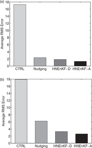
The differences between the HNEnKF with only the diagonal elements of the hybrid nudging magnitude matrix and the HNEnKF with all elements of the hybrid nudging magnitude matrix are first explored. The average RMS errors of CTRL using no data assimilation, traditional nudging and the two HNEnKF approaches during the 3000-step period using both the perfect and imperfect model are shown in Fig. 3. The traditional nudging and HNEnKF approaches produce much smaller average RMS errors than the CTRL. Thus, the results of CTRL will not be shown in the following discussions. Compared to the HNEnKF with all elements of the hybrid nudging magnitude matrix (Experiment HNEnKF-A), the HNEnKF with only diagonal elements of the hybrid nudging magnitude matrix (Experiment HNEnKF-D) produces results closer to the traditional nudging. Nonetheless, the HNEnKF-D has smaller average RMS errors than the traditional nudging. This suggests that there is some advantage to using flow-dependent/time-dependent background error covariance from the ensemble forecast to provide the nudging coefficients. Moreover, the HNEnKF-A has even lower average RMS errors than the HNEnKF-D. Thus, the effectiveness of the HNEnKF-A to extend the nudging magnitude matrix to include inter-variable influences via non-zero off-diagonal elements is also demonstrated. This additional coupling from the inter-variable (off-diagonal) statistics leads to more accurate adjustment of background to the observation than does the traditional nudging method.

Fig. 3.  The average RMS errors for the 3000-step dynamic-analysis period set-up for the control run without data assimilation, traditional nudging and two kinds of HNEnKF approaches described in Table 1 for (a) perfect model and (b) imperfect model.

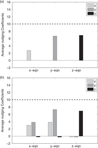
To further demonstrate the effectiveness of the HNEnKF using flow-dependent/time-dependent background error covariance from the ensemble forecast to provide the hybrid nudging coefficients, the average values of the hybrid nudging coefficients of the two HNEnKF approaches are shown in Fig. 4. The diagonal hybrid nudging coefficients are smaller and within an order of magnitude of the traditional nudging coefficients. For Experiment HNEnKF-A (Fig. 4b), the diagonal nudging coefficients are generally larger than the off-diagonal ones, and the off-diagonal coefficients relating to z are much smaller than those off-diagonal elements of x and y. These findings are consistent with the results of Yang et al. (2006). Also note that the off-diagonal terms can be negative because they are not really nudging terms and because the off-diagonal corrections do not directly involve the predictive variable of the equation. Thus, the utility of the EnKF gain matrix to provide time-dependent information to the hybrid nudging coefficients has been demonstrated.

Fig. 4.  The average hybrid nudging coefficients in the 3000-step period set-up in each equation for (a) experiment HNEnKF-D and (b) experiment HNEnKF-A. The dashed line denotes the magnitude of the nudging coefficient used in the traditional nudging approach.

From the discussions above, the HNEnKF schemes have the flow-dependent/time-dependent hybrid nudging coefficients computed from the ensemble forecast. The HNEnKF-A experiment extends the nudging coefficients to non-zero off-diagonal elements and produces smaller average RMS error compared to HNEnKF-D. Therefore, the focus will be on HNEnKF-A from this point forward, and the HNEnKF-A experiment is denoted by HNEnKF in the following sections.

6.2. Sensitivity of the data assimilation methods to observation frequency

In addition to comparing the results from Experiment HNEnKF to other data assimilation approaches in Experiments Nudging, IAU, EnKF and EnKS, the sensitivity of these data assimilation approaches to observation frequency is studied. The comparisons among these data assimilation approaches may vary due to different observation frequencies, since the ensemble spread has different time scales to grow given the different observation frequencies, and the nudging may have difficulties adjusting to the evolving state with more frequent observations. Higher-frequency observations can produce larger observational tendencies that may require the nudging coefficients to be increased for the model to approach a faster evolving observation, and this would violate the important assumption that the nudging terms are relatively small and thus impede the model adjustment process. The default observation frequency used in Section 6.1 is one per 25 time steps. The other observation frequencies used here are one per 10 time steps and one per 50 time steps. The effects of the different data assimilation schemes (Table 1) with different observation frequencies are investigated here within the 3000-step period set-up.

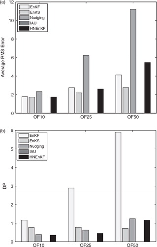
Figure 5a shows the average RMS errors over all time steps for each data assimilation method with different observation frequencies under the perfect model assumption. As discussed earlier, the average RMS error is not the only measurement of success for a dynamic analysis, because it may not best reflect the error spikes or temporal smoothness of the data assimilation. As defined in Section 4, the DP for this group of experiments is also computed, and it is shown in Fig. 5b.

Fig. 5.  The average performance metrics over the 3000-step dynamic-analysis period set-up for the different data assimilation methods described in Table 1 with various observation frequencies of one per 10 time steps (OF10), one per 25 time steps (OF25) and one per 50 time steps (OF50), under a perfect model assumption for (a) RMS error and (b) DP. Smaller values are more desirable for both metrics.

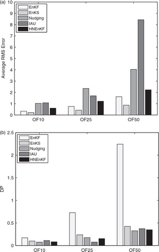
Experiment HNEnKF produces lower RMS errors than Experiment Nudging and IAU for all three observation frequencies, especially when the observation frequency is one per 50 time steps. Thus, the use of flow-dependent/time-dependent nudging coefficients appears to be helpful in reducing the RMS error when the observations are sparse in time. Although Experiment HNEnKF has somewhat larger RMS errors than Experiments EnKF and EnKS, Experiment HNEnKF has closer and similar values of DP to the EnKS and has much smaller values of DP than the intermittent EnKF. The continuous data assimilation experiments, EnKS, Nudging, IAU and HNEnKF, have fewer/smaller discontinuities than the intermittent data assimilation experiment EnKF. Therefore, the HNEnKF combines the advantages of Nudging and EnKF, because it produces smaller RMS errors than the traditional nudging and has better values of DP than the EnKF.

Figure 6 shows the average RMS error and DP for each data assimilation method for the three different observation frequencies within the 3000-step period set-up using an imperfect model (see Section 5). The IAU becomes unstable after adding model errors; therefore, its results are not shown. Bergemann and Reich (2010) also report instability problems with their hybrid IAU method over long data assimilation cycles. Experiment HNEnKF produces lower average RMS errors than traditional nudging, which is similar to the result in the perfect model. The HNEnKF produces similar average RMS errors to the EnKF and EnKS when the observation frequency is one per 10 time steps and one per 25 time steps, but somewhat larger average RMS error for one per 50 steps. One reason that the HNEnKF has somewhat larger average RMS error than the EnKF and EnKS with observation frequency of one per 50 time steps may be: in this highly non-linear Lorenz three-variable model system, the nudging may not perform well when the system is at transitions, 2 since the model state may evolve too quickly to be corrected by the gradual nudging forcing within the nudging time window. However, as shown in Fig. 6b, the HNEnKF has lower values of DP than the EnKF, suggesting smaller discontinuities than the EnKF. Moreover, the HNEnKF has similar or even better DP than the EnKS when the model is imperfect.

Fig. 6.  Same as Fig. 5, except for the imperfect model.

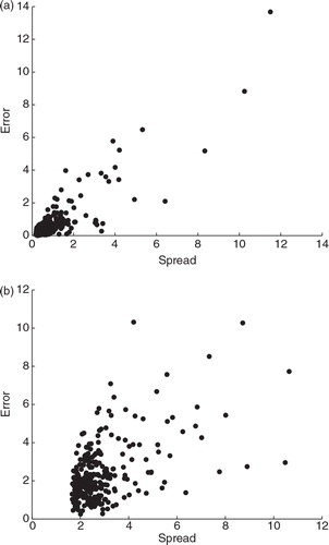
To ensure the EnKF and HNEnKF function properly, the ensemble spread is compared to the forecast error in the EnKF. The ensemble forecast spread and forecast RMS error of the ensemble mean are computed at the observation time but before assimilating the observation. When the observation frequency is one per 25 time steps, the ensemble spread and forecast error are computed every 25 time steps, and their comparisons are shown in Fig. 7. For both perfect and imperfect models, the ensemble spread generally agrees with the forecast error, although the ensemble spread has more variance with the forecast error when the model error is introduced. Generally, the ensemble spread is linearly correlated with the forecast error and the slope of the ‘best-fit’ line is approximately 1. Similar results are obtained for the other observation frequencies (not shown). We conclude that the ensemble spread provides a reasonable estimate of the forecast error in the EnKF and HNEnKF experiments, and, therefore, the EnKF functions with proper ensemble spread.

Fig. 7.  The ensemble spread and error of the 3000-step period set-up using an observation frequency one per 25 time steps. (a) Perfect model and (b) imperfect model.

As discussed in this section, with a perfect model the HNEnKF produces smaller RMS errors than the traditional nudging, although it has somewhat larger RMS errors than the EnKF. Moreover, the HNEnKF has much smaller values of DP than the EnKF and closer values of DP to the EnKS. When model error is introduced, the HNEnKF produces similar RMS errors to the EnKF except when the observation frequency is one per 50 time steps, and it also has much lower values of DP than the EnKF. Therefore, the HNEnKF is able to retain the advantages of the EnKF and produce better temporal smoothness, although it sometimes has somewhat larger RMS errors than the EnKF.

6.3. Sensitivity of the data assimilation methods to initial conditions

Results in Sections 6.1 and 6.2 are based on a 3000-step period set-up as in Yang et al. (2006). However, the results may vary over different periods and different initial conditions. Therefore, a statistical set-up with 100 random initial conditions is performed for both perfect and imperfect models in this section as described in Section 5.

Tables 2 and 3 show the average RMS error and DP of the different data assimilation schemes, with the default observation frequency in the 100 random initial conditions set-up for the perfect model experiment. As shown by Table 2, Experiment HNEnKF under the perfect model assumption produces smaller average RMS errors than traditional nudging and IAU, but larger average RMS errors than the EnKF and the EnKS. A paired Student's t-test is performed to examine if the average RMS errors are significantly different among the data assimilation methods. The null hypothesis is that the two data assimilation methods produce the same average RMS error. A p-value, which is the probability of observing a value at least as extreme as the test statistic under the null hypothesis, less than 0.05 rejects the null hypothesis, indicating that the average RMS error of the data assimilation method in the row is significantly different from that of the data assimilation method in the column. The results of the paired Student's t-test of the average RMS error are also shown in Table 2. The differences among the data assimilation methods are all significant. The Nudging, IAU, HNEnKF and EnKS experiments have significantly better DP than the intermittent data assimilation method EnKF (Table 3). Moreover, the HNEnKF has slightly better, but significantly different DP, than the EnKS as shown in Table 3.

Table 2. The average RMS error in the 100 random initial conditions set-up for the data assimilation methods described in Table 1 with the default observation frequency (one per 25 time steps) for the perfect model

	EnKF	EnKS	Nudging	IAU	HNEnKF
EnKF	0.84	+	+	+	+
EnKS		0.48	+	+	+
Nudging			2.70	+	+
IAU				1.66	+
HNEnKF					1.54

There is significant difference (+) and no significant difference (−).

Table 3. Same as Table 2, except for the DP

	EnKF	EnKS	Nudging	IAU	HNEnKF
EnKF	0.74	+	+	+	+
EnKS		0.20	+	−	+
Nudging			0.22	−	+
IAU				0.20	+
HNEnKF					0.16

Tables 4 and 5 are the same as Tables 2 and 3, except that the results are for the imperfect model. As mentioned in Section 6.2, the IAU becomes numerically unstable when model error is introduced, so its results are not shown. The HNEnKF produces slightly smaller but significantly different average RMS error than either Nudging or EnKF, although it has larger average RMS error than the EnKS (Table 4). Moreover, Table 5 indicates that the HNEnKF has much smaller values of DP than the EnKF and slightly smaller but significantly different values of DP than the EnKS, while the traditional nudging experiment (Nudging) produces the best values of DP. Therefore, the results obtained in the 100 random initial conditions set-up in this section are generally consistent with those in the 3000-step period set-up as discussed in Section 6.2. Moreover, the results from this section based on the paired Student's t-test with a 95% confidence level demonstrate that the conclusions from the 3000-step period set-up (Section 6.2) are generally valid.

Table 4. Same as Table 2, except for the imperfect model

	EnKF	EnKS	Nudging	IAU	HNEnKF
EnKF	2.73	+	−		+
EnKS		1.87	+		+
Nudging			3.01		+
IAU
HNEnKF					2.64

Table 5. Same as Table 4, except for the DP

	EnKF	EnKS	Nudging	IAU	HNEnKF
EnKF	2.96	+	+		+
EnKS		0.58	+		+
Nudging			0.36		+
IAU
HNEnKF					0.50

6.4. Nudging coefficients constraints

The underlying assumption for nudging, as stated by Stauffer and Seaman (1990, 1994), is that the nudging terms should be constrained to be smaller than the model's physical terms in order to retain the physical properties and dynamic balance/inter-variable consistency of the system. For this highly non-linear Lorenz three-variable model system, the nudging terms may need to be larger when the system is at transitions. The synchronisation of the master (truth run) with the slave (model with coupling/nudging terms) in Yang et al. (2006), using a coupling strength that varies from 1 to 100, may violate this assumption. Thus, the nudging coefficient constraints for the HNEnKF are investigated further here.

Figure 8 shows the average ratios of the nudging terms over the sum of the physical terms in each equation in the 3000-step period set-up of HNEnKF under the perfect model assumption. The ratio of the y nudging term in the y-equation is 0.13, which is slightly larger than 0.1 (an order of magnitude difference in the magnitudes of the nudging term and physical terms). The other nudging terms have ratios smaller than 0.1.

Fig. 8.  The average ratios of the hybrid nudging terms in each equation compared with the sum of the physical terms for the 3000-step period set-up for Experiment HNEnKF. The dashed line denotes a ratio of 0.1, where the nudging term is an order of magnitude smaller than the sum of the physical forcing terms.

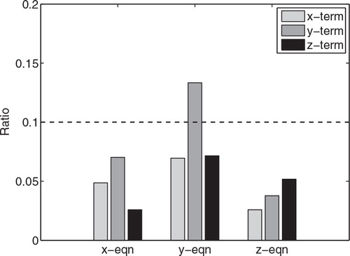
Thus Experiment HNEnKF is generally able to make small and effective innovations to the model background to correct the model trajectory, as shown by the smaller average RMS errors compared to the Experiment Nudging. It can also minimise the insertion noise and produce smaller (better) DP compared to the EnKF. Any nudging-type approach, including our HNEnKF should consider the magnitude of the nudging terms relative to the physical forcing terms, so that dynamic balance and consistency are retained in addition to reducing the RMS errors compared to the truth state. Hollingsworth et al. (1986) discussed a similar criterion, which requires the magnitude of the analysis increment to be smaller than that of the forecast increment.

6.5. Computational efficiency

The HNEnKF experiment is shown to produce similar or slightly better average RMS errors to the EnKF for the imperfect model but better DP than the EnKF in general. It also produces similar or even better values of DP compared to the gold standard EnKS. However, the EnKS is much more CPU-intensive than the HNEnKF and also requires greater storage proportional to the total number of analysis times over which the statistics are to be applied. Although all the EnKF, HNEnKF and EnKS experiments have an ensemble forecast that is more expensive than a single model run as used in Experiments Nudging and IAU, the EnKS applies future observations backward to the initial time, which adds even more computational cost for calculating the temporal error correlations compared with the EnKF and HNEnKF. This is also the reason that the EnKS requires greater storage than the EnKF and HNEnKF – the ensemble spread at each analysis time (here every time step) needs to be stored and is used to compute the temporal error correlations.

Table 6 shows the CPU time cost of the various data assimilation schemes with the default observation frequency in the 100 random initial conditions set-up. The Nudging and IAU experiments have the smallest CPU time cost, because they do not include an ensemble forecast. The HNEnKF has similar CPU time cost to the EnKF, but the EnKS has a CPU time cost more than 200 times that of the EnKF and HNEnKF. Thus, the HNEnKF produces somewhat larger average RMS error than the EnKS and similar or better DP to the EnKS, but with substantially reduced CPU time and storage costs.

Table 6. Total CPU time cost of different data assimilation schemes with the default observation frequency in the 100 initial conditions set-up

Experiment	EnKF	EnKS	Nudging	IAU	HNEnKF
CPU time (s)	16	3414	4	5	16

7. Conclusions

A new HNEnKF data assimilation approach that produces time-continuous, seamless dynamic analyses over a fixed period is explored here using the Lorenz three-variable system with both perfect and imperfect models. The HNEnKF approach allows the EnKF to be applied gradually in time via nudging-type terms. The flow-dependent, time-varying error covariance matrix is used to compute the nudging coefficients rather than using ad hoc values derived from theory and experience. The HNEnKF using all elements of the nudging magnitude matrix produces better results than the HNEnKF using only the diagonal elements of the nudging magnitude matrix, because it allows for greater inter-variable influences from the data assimilation via the non-zero off-diagonal elements of the nudging magnitude matrix.

The HNEnKF approach promotes a better fit to the data compared to traditional nudging or IAU while also minimising the error spikes or bursts created by intermittent assimilation methods such as the EnKF. When model error is introduced, the HNEnKF still produces lower average RMS errors than the traditional nudging and closer or better average RMS errors compared to the EnKS and EnKF, respectively. The ensemble spread provides a reasonable estimate of the forecast error in the EnKF and HNEnKF experiments. The HNEnKF also produces better DP than the EnKF and even better DP than the EnKS. The EnKS, as the gold standard, is much more computationally expensive and has larger storage requirements. The EnKS requires more than 200 times more CPU time than the EnKF and HNEnKF used in this study.

Although the HNEnKF is comparable in cost to the EnKF, it offers a gradual, continuous assimilation of the data with better inter-variable consistency, improved temporal smoothness and reduced noise levels between the observation times compared to the EnKF. The hybrid nudging terms in the HNEnKF are on average an order of magnitude smaller than the physical terms in all three equations. Any nudging-type approach should not use nudging terms that are relatively large compared to the physical forcing terms, so that dynamic balance and consistency are retained in addition to reducing the RMS errors compared to the truth state.

The advantages of the HNEnKF demonstrated in the Lorenz three-variable system motivated us to further explore this HNEnKF approach in a more realistic two-dimensional shallow-water model system in Part II (Lei et al., 2012). Building on the encouraging results obtained from this two-part study using simplified models, we will apply the HNEnKF to the three-dimensional WRF model. The results will be presented in another paper (accepted by Q. J. R. Meteorol. Soc.).

Acknowledgements

This research was supported by DTRA contract No. HDTRA1-07-C-0076 under the supervision of John Hannan of DTRA. The authors would like to thank Aijun Deng and Fuqing Zhang for helpful discussions and comments.

Notes

¹The signal to noise ratio is the variance of the variable divided by its observation error variance.

²The “transitions” mean the locations that are very sensitive to error, where a small amount of error may lead the model state to a different fixed point.

References

- Anderson J. L. An ensemble adjustment Kalman filter for data assimilation. Mon. Weather Rev. 2001; 129: 2884–2903.
- Auroux D. Blum J. A nudging-based data assimilation method: the back and forth (BFN) algorithm. Nonlin. Process. Geophys. 2008; 15: 305–319. 10.3402/tellusa.v64i0.18484.
- Ballabrera-Poy J. Kalnay E. Yang S. Data assimilation in a system with two scales — combining two initialization techniques. Tellus. 2009; 61A: 539–549.
- Bergemann K. Reich S. A mollified ensemble Kalman filter. Q. J. R. Meteorol. Soc. 2010; 136: 1636–1643. 10.3402/tellusa.v64i0.18484.
- Bishop C. H. Etherton B. J. Majumdar S. J. Adaptive sampling with the ensemble transform Kalman filter. Part I: theoretical aspects. Mon. Weather Rev. 2001; 129: 420–436.
- Bloom S. C. Takacs L. L. da Silva A. M. Ledvina D. Data assimilation using incremental analysis updates. Mon. Weather Rev. 1996; 124: 1256–1271.
- Chin T. M. Turmon M. J. Jewell J. B. Ghil M. An ensemble-based smoother with retrospectively updated weights for highly nonlinear system. Mon. Weather Rev. 2007; 135: 186–202. 10.3402/tellusa.v64i0.18484.
- Cohn S. Sivakumaran N. S. Todling R. A fixed-lag Kalman smoother for retrospective data assimilation. Mon. Weather Rev. 1994; 122: 2838–2867.
- Courtier, P, Anderson, E, Heckley, W, Pailleux, J, Vasiljevic, D and co-authors. 1998. The ECMWF implementation of three-dimensional variational assimilation (3D-Var). Part I: formulation. Q. J. R. Meteorol. Soc. 124, 1783–1808.
- Deng A. Seaman N. L. Hunter G. K. Stauffer D. R. Evaluation of interregional transport using the MM5-SCIPUFF system. J. Appl. Meteorol. 2004; 43: 1864–1886. 10.3402/tellusa.v64i0.18484.
- Deng A. Stauffer D. R. On improving 4-km mesoscale model simulations. J. Appl. Meteorol. 2006; 45: 361–381. 10.3402/tellusa.v64i0.18484.
- Dixon M. Li Z. Lean H. Roberts N. Ballard S. Impact of data assimilation on forecasting convection over the United Kingdom using a high-resolution version of the Met office unified model. Mon. Weather Rev. 2009; 137: 1562–1584. 10.3402/tellusa.v64i0.18484.
- Duane G. S. Tribbia J. J. Weiss J. B. Synchronicity in predictive modeling: a new view of data assimilation. Nonlin. Process. Geophys. 2006; 13: 601–612. 10.3402/tellusa.v64i0.18484.
- Evensen G. Sequential data assimilation with a nonlinear quasi-geostrophic model using Monte Carlo methods to forecast error statistics. J. Geophys. Res. 1994; 99(C5): 10143–10162. 10.3402/tellusa.v64i0.18484.
- Evensen G. Advanced data assimilation for strongly nonlinear dynamics. Mon. Weather Rev. 1997; 125: 1342–1354.
- Evensen G. van Leeuwen P. J. An ensemble Kalman smoother for nonlinear dynamics. Mon. Weather Rev. 2000; 128: 1852–1867.
- Friedrichs K. The identity of weak and strong extensions of differential operators. Trans. Am. Math. Soc. 1944; 55: 132–151.
- Fujita T. Stensrud D. J. Dowell D. C. Surface data assimilation using an ensemble Kalman filter approach with initial condition and model physics uncertainties. Mon. Weather Rev. 2007; 135: 1846–1868. 10.3402/tellusa.v64i0.18484.
- Hamill T. M. Snyder C. A hybrid ensemble Kalman filter-3D variational analysis scheme. Mon. Weather Rev. 2000; 128: 2905–2919.
- Hoke J. E. Anthes R. A. The initialization of numerical models by a dynamical initialization technique. Mon. Weather Rev. 1976; 104: 1551–1556.
- Hollingsworth, A, Shaw, D. B, Lönnberg, P, Illari, L, Arpe, K and co-authors. 1986. Monitoring of observation and analysis quality by a data assimilation system. Mon. Weather Rev. 114, 861–879.
- Houtekamer P. L. Mitchell H. L. Data assimilation using an ensemble Kalman filter technique. Mon. Weather Rev. 1998; 126: 796–811.
- Hunt, B. R, Kalnay, E, Kostelich, E. J, Ott, E, Patil, D. J and co-authors. 2004. Four-dimensional ensemble Kalman filtering. Tellus. 56A, 273–277.
- Juckes M. Lawrence B. Inferred variables in data assimilation: quantifying sensitivity to inaccurate error statistics. Tellus. 2009; 61A: 129–143.
- Kalata, P. R. 1984. The tracking index: a generalized parameter for α-β and α-β-γ target trackers. IEEE Trans. Aeros. Electron. Syst. AES-20, 174–182. 10.3402/tellusa.v64i0.18484.
- Khare S. P. Anderson J. L. Hoar T. J. Nychka D. An investigation into the application of an ensemble Kalman smoother to high-dimensional geophysical systems. Tellus. 2008; 60A: 97–112.
- Lee M.-S. Kuo Y.-H. Barker D. M. Lim E. Incremental analysis updates initialization technique applied to 10-km MM5 and MM5 3DVAR. Mon. Weather Rev. 2006; 134: 1389–1404. 10.3402/tellusa.v64i0.18484.
- Lei, L, Stauffer, D. R and Deng, A. 2012. A hybrid nudging-ensemble Kalman filter approach to data assimilation. Part II: application in a shallow-water model. Tellus A 2012, 64, 18485,http://dx.doi.org/10.3402/tellusa.v64i0.18485.
- Leidner S.M. Stauffer D. R. Seaman N. L. Improving short-term numerical weather prediction in the California coastal zone by dynamic initialization of the marine boundary layer. Mon. Weather Rev. 2001; 129: 275–294.
- Liu C. Xiao Q. Wang B. An ensemble-based four-dimensional variational data assimilation scheme. Part I: technical formulation and preliminary test. Mon. Weather Rev. 2008; 136: 3363–3373. 10.3402/tellusa.v64i0.18484.
- Lorenc A. C. Analysis methods for numerical weather prediction. Q. J. R. Meteorol. Soc. 1986; 112: 1177–1194. 10.3402/tellusa.v64i0.18484.
- Lorenz E. Deterministic non-periodic flow. J. Atmos. Sci. 1963; 20: 130–141.
- Otte T. L. The impact of nudging in the meteorological model for retrospective air quality simulations. Part I: evaluation against national observation networks. J. Appl. Meteorol. Climatol. 2008a; 47: 1853–1867. 10.3402/tellusa.v64i0.18484.
- Otte T. L. The impact of nudging in the meteorological model for retrospective air quality simulations. Part II: evaluating collocated meteorological and air quality observations. J. Appl. Meteorol. Climatol. 2008b; 47: 1868–1887. 10.3402/tellusa.v64i0.18484.
- Otte T. L. Seaman N. L. Stauffer D. R. A heuristic study on the importance of anisotropic error distribution in data assimilation. Mon. Weather Rev. 2001; 129: 766–783.
- Ourmieres Y. Brankart J.-M. Berline L. Brasseur P. Verron J. Incremental analysis update implementation into a sequential ocean data assimilation system. J. Atmos. Ocean. Technol. 2006; 23: 1729–1744. 10.3402/tellusa.v64i0.18484.
- Painter J. H. Kerstetter D. Jowers S. Reconciling steady-state Kalman and Alpha-Beta filter design. IEEE Trans. Aerosp. Electron. Syst. 1990; 26: 986–991. 10.3402/tellusa.v64i0.18484.
- Pu Z. Hacker J. Ensemble-based Kalman filters in strongly nonlinear dynamics. Adv. Atmos. Sci. 2009; 26: 373–380. 10.3402/tellusa.v64i0.18484.
- Sasaki Y. Some basic formalisms on numerical variational analysis. Mon. Weather Rev. 1970; 98: 875–883.
- Schroeder, A. J, Stauffer, D. R, Seaman, N. L, Deng, A, Gibbs, A. M and co-authors. 2006. An automated high-resolution, rapidly relocatable meteorological nowcasting and prediction system. Mon. Weather Rev. 134, 1237–1265. 10.3402/tellusa.v64i0.18484.
- Seaman N.L. Stauffer D. R. Lario-Gibbs A. M. A multi-scale four-dimensional data assimilation system applied in the San Joaquin Valley during SARMAP. Part I: modeling design and basic performance characteristics. J. Appl. Meteorol. 1995; 34: 1739–1761.
- Stauffer D. R. Bao J.-W. Optimal determination of nudging coefficients using the adjoint equations. Tellus. 1993; 45A: 358–369.
- Stauffer D. R. Seaman N. L. Use of four-dimensional data assimilation in a limited-area mesoscale model. Part I: experiments with synoptic data. Mon. Weather Rev. 1990; 118: 1250–1277.
- Stauffer D. R. Seaman N. L. Multiscale four-dimensional data assimilation. J. Appl. Meteorol. 1994; 33: 416–434.
- Stauffer D. R. Seaman N. L. Binkowski F. S. Use of four-dimensional data assimilation in a limited-area mesoscale model. Part II: effects of data assimilation within the planetary boundary layer. Mon.Weather Rev. 1991; 119: 734–754.
- Stauffer, D. R, Seaman, N. L, Hunter, G. K, Leidner, S. M, Lario-Gibbs, A and co-authors. 2000. A field-coherence technique for meteorological field-program design for air quality studies. Part I: description and interpretation. J. Appl. Meteorol. 39, 297–316.
- Tanrikulu S. Stauffer D. R. Seaman N. L. Ranzieri A. J. A field-coherence technique for meteorological field-program design for air-quality studies. Part II: evaluation in the San Joaquin Valley. J. Appl. Meteorol. 2000; 39: 317–334.
- Thepaut J.-N. Hoffman R. Courtier P. Interactionsof dynamics and observations in a four-dimensional variational data assimilation. Mon. Weather Rev. 1993; 121: 3393–3414.
- Wang X. Baker D. M. Snyder C. Hamill T. M. A hybrid ETKF-3DVAR data assimilation scheme for the WRF model. Part I: observing system simulation experiment. Mon. Weather Rev. 2008a; 136: 5116–5131. 10.3402/tellusa.v64i0.18484.
- Wang X. Baker D. M. Snyder C. Hamill T. M. A hybrid ETKF-3DVAR data assimilation scheme for the WRF model. Part II: real observation experiments. Mon. Weather Rev. 2008b; 136: 5132–5147. 10.3402/tellusa.v64i0.18484.
- Whitaker, J. S and Compo, G. P. 2002. An ensemble Kalman smoother for reanalysis. In: Proceedings of Symposium on Observations, Data Assimilation and Probabilistic Prediction, Orlando, FL, AMS, 144–147.
- Whitaker J. S. Hamill T. M. Ensemble data assimilation without perturbed observations. Mon. Weather Rev. 2002; 130: 1913–1924.
- Yang, S, Baker, D, Li, H, Cordes, K, Huff, M and co-authors. 2006. Data assimilation as synchronization of truth and model: experiments with the three variable Lorenz system. J. Atmos. Sci. 63, 2340–2354. 10.3402/tellusa.v64i0.18484.
- Zou X. Navon I. M. Ledimet F. X. An optimal nudging data assimilation scheme using parameter estimation. Q. J. R. Meteorol. Soc. 1992; 118: 1163–1186. 10.3402/tellusa.v64i0.18484.