On the variability of projected tropical cyclone genesis in GCM ensembles

ABSTRACT

The development of projections for changes in the genesis of tropical cyclones (TCs) for a changed climate is explored in this article using outputs from the Coupled Model Intercomparison Project: Phase 3 (CMIP3) models. In this study, we explore how the projected change in the genesis frequency of TCs strongly depends upon the selection of models used in the ensemble. Results from 16 CMIP3 models are analysed and validated against the National Center for Environmental Prediction (NCEP) and European Centre for Medium Range Weather forecast re-analysis at 40 km (ERA40) reanalysis and an ensemble mean of TC genesis diagnostics is calculated using the CMIP3 models. The response of these models to a future climate using the IPCC A2 scenario is also studied in the context of selecting models to calculate an ensemble mean.

• tropical cyclone
• genesis potential index (GPI)
• CMIP3
• ensemble
• climate change

1. Introduction

Tropical cyclones (TCs) are severe weather phenomena which have a devastating effect in terms of loss of life and economy and have been identified as the most costly disaster in the USA by Peterson et al. (2008). An increased severity of TCs or hurricanes in the North Atlantic for the past 30 yr has been reported in the literature (Webster et al., 2005; Emanuel, 2005) with many studies (Trenberth and Shea 2006; Holland and Webster, 2007) attributing this change to human-induced global warming. However, this view has been challenged by others (Landsea, 2007) who relate the changes to discrepancies in the available observations. The impact of TCs in the context of future climate is very important because projection of any change in the frequency, intensity and location of TCs will help communities to plan and adapt to future climate. Knutson et al. (2010) have recently reported that based on theory and high resolution dynamical modelling, the globally averaged intensity of TCs will become stronger due to greenhouse gas (GHGs) warming. They also report a projected decrease in the globally averaged frequency of TCs by existing modelling studies. Villarini et al. (2011) have developed a statistical model to study the change in TC frequency due to increases in future GHGs. They report that the dominant drivers of uncertainty in projections of tropical storm frequency, intensity and location over the 21st-century are internal climate variations and systematic inter-model differences in the response of sea surface temperature (SST) patterns to increasing GHGs.

A number of projects have previously studied TCs using Global Climate Model (GCM) outputs. However, it is recognised that GCMs have difficulty in representing the climatology of TCs due to the low resolution of the models as well as deficiencies in their representation of the characteristics of large-scale drivers such as El Nino Southern Oscillation (ENSO), the monsoon and the South Pacific Convergence Zone. To diagnose TC formation, large-scale environmental factors are used to build empirical indices that replicate the key features of cyclogenesis. For example, one of the earliest indices, the Yearly Genesis Parameter (YGP) (Gray, 1979), has been used in studies by Ryan et al. (1992) and Watterson et al. (1995). Royer et al. (1998) showed that the YGP could not be used to address climate change and refined this index by modifying the thermal component of the index through the use of convective precipitation. This convective yearly genesis parameter (CYGP) has been used recently to address climate change impacts on TCs in studies by Chauvin et al. (2006) and Caron and Jones (2008). Emanuel and Nolan (2004) have proposed the genesis potential index (GPI) which was developed based on National Center for Environmental Prediction (NCEP) reanalysis data. The GPI uses the concept of potential intensity (Bister and Emanuel, 1998) to account for thermal conditions. The GPI has been used in a number of studies to infer cyclogenesis in reanalysis data as well as in GCMs (e.g. Camargo et al., 2007b).

Vecchi and Soden (2007), Caron and Jones (2008) and Zhang et al. (2010) have studied the impact of global warming on TCs in future climate scenarios using outputs from the Coupled Model Intercomparison Project: Phase 3 (CMIP3) outputs. Vecchi and Soden (2007) analysed the change in GPI and maximum potential intensity (MPI) indices for the IPCC SRES A1B scenario while Caron and Jones (2008) used the CYGP to study its change in three scenarios, B1, A1B and A2. Zhang et al. (2010) have used only two models to diagnose the change in GPI for the late–21st-century climate using results for the A2 scenario and found an increase in GPI for the Western North Pacific basin. However, a comparison of the results from Vecchi and Soden (2007) and Caron and Jones (2008) shows marked differences in the projected pattern of change for the TC genesis parameter indices for the A1B scenario as well as B1 scenario. The difference between the studies may be attributed to the different indices used in the studies, different time slices used or to the different model ensembles used to calculate the projections.

Caron and Jones (2008) used the same periods for the current and future climates and the same emissions scenario as the present study; however, they used the CYGP to calculate genesis. A recent study by Menkes et al. (2012) has compared four different climate indices, including the GPI and CYGP. Although the two indices use different parameters to calculate cyclogenesis, the underlying principles used in the calculation of these indices are similar, although Menkes et al. (2011) found that the mean simulated genesis numbers exhibit large regional variations which can reach up to ±50%. Chauvin and Royer (2010) have also compared the differences in the response of GCMs due to IPCC A2 scenario using both the GPI and CYGP techniques. They found that the overall response of the two indices for individual models have similar patterns; however, their magnitudes vary (Chauvin and Royer, 2010; Figs. 2 and 3). Thus, in this study, we explore how the projected change in the genesis frequency of TCs is affected by the selection of models used in the ensembles chosen to represent the late–20th- and 21st-century climates, rather than investigating the differences due to choice of genesis index. In addition, Caron and Jones (2008) do not use paired samples in their calculations of late–20th- and 21st-century climates, thus in this article we compare the response of the models when paired and unpaired samples are used.

In this article, outputs from the IPCC AR4 models have been analysed to infer cyclogenesis using the GPI for the 20th-century simulations and for the A2 scenario for the late–21st-century. The A2 scenario was chosen as this is the most extreme GHG warming scenario for which the data required to calculate the projected change in GPI were available. Caron and Jones (2008) used the CYGP to calculate the projected change in TC genesis for three scenarios, B1, A1B and A2. Their results show that the pattern of change remains the same for each of the scenarios; however, the change becomes stronger as the scenarios become more extreme.

Four different ensembles were created with different models for the late–20th- and late–21st-century climates based on Caron and Jones (2008). Statistical analysis of the results shows the importance of selecting paired samples when calculating the difference in GPI between two time periods. The experimental design, model description and analysis techniques are detailed in Section 2. In Section 3, the results from the analysis are presented. This is followed by discussion and conclusion in Section 4.

2. Data and analysis method

A detailed description of the analysis method and the models used in this study are described in this section.

The GPI can be expressed as:1

where , , and .

The term PI is the potential intensity of the cyclonic wind speed that might be attainable under the given SST and thermodynamic conditions; it is based on the formulation of Emanuel (1995) and calculated using the code obtained from the following link (ftp://texmex.mit.edu/pub/emanuel/TCMAX/pcmin_revised.f). The variables used to calculate the PI are SST and pressure and vertical profiles of temperature and specific humidity. The term ∣U ₂₀₀−U ₈₀₀∣ is the magnitude of the vertical wind shear, RH₇₀₀ is the relative humidity at 700 hPa and Vort₈₅₀ is the absolute vorticity at 850 hPa. This index is suitable to use for the calculation of TC frequencies for future climate as there are no threshold values used in the calculation of its thermodynamic component (Camargo et al., 2007a).

Models initially selected for this study were chosen based upon the availability of daily data with 17 models providing suitable outputs. However, a comparison of GPI calculated for individual models using daily outputs differed from those of Chauvin and Royer (2010). This was traced to differences in GPI calculated using nine-level daily data in comparison to that calculated using the 17 levels available for monthly data. Thus, the GPI calculations used here are based upon the 17-level monthly data fields. Note that although daily outputs were available for MUIB_ECHO_G, it was not included in this study as monthly outputs were unavailable for this model.

Twenty years of outputs from 1981 to 2000 were used to analyse the late–20th-century TC frequency for all 16 models and their ensemble average is compared with a similar analysis based on NCEP and ERA40 reanalysis data for the same period. A further 20 yr of data from 2081 to 2100 for the A2 scenario were used to calculate the GPI for the late–21st-century. The projected change in TC frequency is the difference between the results for 2081–2100 and 1981–2000.

In order to test the effect of sampling of the GCMs on the GPI and its change for a future climate scenario, a number of ensembles were created and are shown in Table 2. Ensemble E-I uses a single realisation from all 16 models as stated in Table 1 to calculate the GPI for both scenarios 20c3m and A2. Ensemble E-II comprises the same models used in the study by Caron and Jones (2008). Note that E-II does not have all the models included in E-I, it uses multiple realisations of some models in the 20th-century and it uses a different set of models for scenario A2. Specifically, scenario 20c3m uses three realisations for ECHAM5, GFDL-CM-2.0, GFDL-CM-2.1 and MRI_CGCM2 and two realisations for HADGEM1 while scenario A2 considers two realisations for ECHAM5 and MRI_CGCM2 and none for MIROC_MEDRES and CCCMA. In order to treat the models with multiple realisations with the same weighting as the models with a single realisation, an ensemble mean GPI of the models with multiple realisations is used to create Ensemble E-III. All members of the ensemble are paired except CCMA and MIROC_MEDRES which do not have any representation in Scenario A2. For Ensemble E-IV, the models which do not have their corresponding representative in the 21st-century have been excluded from the current climate. Hence, CCCMA and MIROC_MEDRES are excluded from the Scenario 20c3m as they do not have any representation in Scenario A2. Ensemble E-V is created using the same set of models as E-I, but a mean GPI is used for the models belonging to the same family (e.g. CSIRO-Mk3.0 and CSIRO-Mk3.5, GFDL-CM-2.0 and GFDL-CM-2.1 and UKMO-HadCM3 and UKMO-HadGEM1).

Table 1. List of the 16 GCMs used in the analysis of GPI for the late–20th and 21st-century

Model	Abbreviation	Country of origin	Reference
BCCR-BCM2.0	BCCR	Norway	Furevik et al. (2003)
CGCM3.1	CCCMA	Canada	Flato et al. (2000)
CNRM-CM3	CNRM	France	Salas-Melia et al. (2005)
CSIRO-Mk3.0	CSIRO_Mk_3.0	Australia	Gordon et al. (2002)
CSIRO-MK3.5	CSIRO_Mk_3.5	Australia	Gordon et al. (2002)
ECHAM5-MPI	ECHAM5	Germany	Roeckner et al. (2003)
GFDL-CM2.0	GFDL2.0	USA	Delworth et al. (2006)
GFDL-CM2.1	GFDL2.1	USA	Delworth et al. (2006)
GISS-MODEL-ER	GISS_ER	USA	Schmidt et al. (2006)
UKMO-HadCM3	HadCM3	UK	Johns et al. (2004)
UKMO-HadGEM1	HadGEM1	UK	Johns et al. (2004)
INGV-ECHAM4	ECHAM4	Italy	Roeckner et al. (2003)
INMCM3	INMCM3	Russia	Galin et al. (2003)
IPSL-CM4	IPSL	France	Marti et al. (2005)
MIROC-medres	MIROC	Japan	K-1 Model developers (2004)
MRI-CGCM2.3.2	MRI	Japan	Yukimoto and Noda (2003)

3. Results and discussion

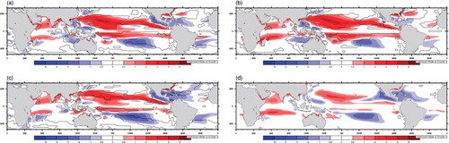
The GPI is calculated for all 16 GCMs as listed in Table 2 (E-I) using their monthly averaged data. The monthly values were used to calculate four seasonal averages of GPI (January–February–March, April–May–June, July–August–September and October–November–December) and these seasonal averages combined to create an annual average GPI. The annual ensemble average of GPI for E-I and the GPI calculated from NCEP and ERA40 reanalysis data are shown in Fig. 1.

Fig. 1.  Annual mean GPI for the late–20th-century climate: (a) ERA40 reanalysis, (b) NCEP reanalysis, (c) GPI: E-I mean, (d) E-I SD and (e) the COV of GPI for E-I. Units for (a)–(d) are number of cyclogenesis per 2.5° per 20 yr.

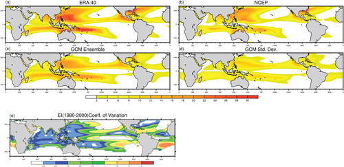
Table 2. List of GCMs used in the construction of various ensembles for the current climate and IPCC AR4 A2 scenario and ensemble names

	Scenario 20c3m					Scenario A2
Model	EI	EII	EIII	EIV	EV	EI	EII	EIII	EIV	EV
BCCR	1	1	1	1	1	1	1	1	1	1
CCCMA	1	1	1	0	1	1	0	0	0	1
CNRM	1				1	1				1
CSIRO3.5	1	1	1	1	Mean	1	1	1	1	Mean
CSIRO3.0	1					1
ECHAM5	1	3	Mean	Mean	1	1	2	Mean	Mean	1
GFDL2.0	1	3	Mean	Mean	Mean	1	1	1	1	Mean
GFDL2.1	1	3	Mean	Mean		1	1	1	1
GISS-ER	1				1	1				1
MIROC	1	1	1	0	1	1	0	0	0	1
MRI	1	3	Mean	Mean	1	1	2	Mean	Mean	1
HadGEM1	1	2	Mean	Mean	Mean	1	1	1	1	Mean
HadCM3	1					1
ECHAM4	1				1	1				1
INMCM3	1				1	1				1
IPSL	1				1	1				1
Total	16	18	9	7	13	16	9	7	7	13

The E-I mean of GPI has similar spatial features when compared against NCEP and ERA40 reanalysis; however, there is significant variation between the models in the values of the GPI as shown by the standard deviation (SD) of the GPI shown in Fig. 1d and the coefficient of variation (COV) shown in Fig. 1e. The difference in the values of GPI between the ERA40 and NCEP reanalyses is likely due to a dry bias in the NCEP relative humidity term which has been noted in studies, such as Bony et al. (1997) and Dessler and Davis (2010). The regions of cyclogenesis in the western North Pacific and Atlantic are similar for the GCM ensemble, NCEP reanalysis and ERA40 reanalysis; however, the basin average values of GPI in the western North Pacific region is approximately 28 for the ERA40 reanalysis and approximately 24 for both NCEP and E-I. In the Southern Hemisphere, similar patterns of cyclogenesis are evident for three cases. The region of enhanced cyclogenesis near the South Pacific Convergence Zone is well simulated by the model ensemble when compared to the two reanalysis datasets. However, the magnitude of the GPI is very different for all three cases in the South Pacific; ERA40 shows a basin average value of approximately 26, the NCEP reanalysis has a value of approximately 22 and E-I a has a value of approximately 24.

The GPI in all 16 models in E-I have very different magnitudes but have similar genesis regions. This feature can be observed in the E-I SD as shown in Fig. 1d. The COV between the models is largest in Central Pacific, North Atlantic and South Pacific basins as shown in Fig. 1e and noted by Yokoi et al. (2009), Zhang et al. (2010) and Camargo et al. (2007b). Emanuel et al. (2008) illustrated that the models have differences in the mean temperature and humidity profiles which depend on their respective convection schemes and these also differ from observations. These differences affect the magnitude of the GPI which was originally formulated based on NCEP reanalysis data. Yokoi et al. (2009) have therefore argued that the focus should be on the horizontal distribution of the GPI rather than its magnitude.

In order to estimate the inter-model difference in GPI, the annual mean of the four components of GPI are calculated for seven ocean basins (North Atlantic, North East Pacific, North West Pacific, Indian Ocean, South Indian Ocean, Western Australia and South Pacific). The values for the individual basins are added and shown in Table 3. Annual GPI is the product of the four components. The COV shows that GPI_3 which represents the MPI component, has the largest value followed by GPI_2 which represents the relative humidity component. These two components have the largest contribution to the variability of GPI which has a COV value of 0.5.

Table 3. Annual mean of the GPI and its four components, added over seven ocean basins

Model	Gpi_1	Gpi_2	Gpi_3	Gpi_4	Gpi
BCCR_BCM2	20.8	2.3	1.58	0.55	40.51
CCCMA	20.3	1.8	2.08	0.53	39.47
CNRM	20.6	2.4	1.31	0.55	35.43
CSIRO3.0	20.1	2.4	0.89	0.55	23.31
CSIRO3.5	20.2	2.4	1.01	0.53	24.24
ECHAM5	20.6	3.6	2.77	0.58	116.66
GFDL2.0	19.9	2.6	1.53	0.55	42.97
GFDL2.1	20.2	2.7	1.36	0.58	42.24
GISS_E-R	19.7	2.9	1.06	0.59	35.77
MIROC	19.7	2.9	1.50	0.52	45.04
MRI	20.4	2.0	1.75	0.56	40.81
HADGEM1	20.5	2.0	1.35	0.56	31.41
HADCM3	20.5	2.5	1.83	0.53	49.84
ECHAM4	20.9	2.3	1.95	0.62	59.18
INMCM3	20.5	1.5	1.68	0.61	30.82
IPSL	19.3	2.6	1.32	0.52	34.43
Coefficient of variation	0.02	0.2	0.3	0.05	0.5

Values are presented for all models.

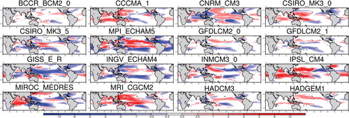
A similar analysis for E-I was carried out for a future climate scenario based on the A2 scenario for 2081–2100 (figure not shown). Similar to the current climate results, there is a lot of variability amongst the models especially in the Western North Pacific and South Pacific regions. The difference between the late–21st-century climate (2081–2100) and late–20th-century climate (1981–2000) is calculated for all the models in E-I and is shown in Fig. 2. There are significant differences in the climate change response of GPI for the models in E-I. This is true, especially over the Central Pacific, South Pacific and Western Australia basins where some models show an increase in the GPI while the others show a decrease.

Fig. 2.  Annual change in GPI for the late–21st-century (2081–2100 minus 1981–2000) for the A2 scenario for the 16 CMIP3 models of E-I.

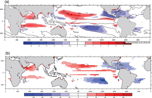
The ensemble mean change in the GPI for future climate, shown in Fig. 3a, shows that, on average, there is an overall increase in GPI in the North Central Pacific and an overall decrease in the East Pacific, North Atlantic and Central South Pacific basins. Of the models, 75% or more agree on the area of decrease in the GPI over the East Pacific, North Atlantic and Central South Pacific basins (Biasutti and Giannini, 2006). The large area of increase in GPI projected for the North Central Pacific is not consistent across models with less than 75% of models projecting an increase for this region. It should be noted that our region of inter-model agreement differ from those of Caron and Jones (2008) due to different samples used in the two studies. The change in GPI was normalised by dividing the change in GPI by its late–20th-century value. The normalised change, shown in Fig. 3b, demonstrates that the largest relative changes as projected by more than 75% of models are found in the Central South Pacific and Northern Indian Oceans.

Fig. 3.  (a) Ensemble average of annual change in GPI for the late–21st-century (2081–2100 minus 1981–2000) for E-I for the A2 scenario with contours showing where 75% of models agree on the sign of change, and (b) normalised change for this same period.

In an effort to understand the effect of using different models to build various ensembles, the analysis was repeated using the same ensemble members as reported by Caron and Jones (2008) for 1981–2000 and 2081–2100 and defined as E-II in Table 2. It should be noted that the Caron and Jones (2008) study used a 1981–2000 climate ensemble of 18 members drawn from nine models and a 2081–2100 climate ensemble of nine members drawn from seven models. In addition, they weighted the models so that the late–20th-century global mean value of GPI was 85. The GPI for the late–20th-century climate is calculated from the list of models in Table 2 for E-II, E-III, E-IV and E-V. Difference between the ensembles and E-I shows that model mean GPI values are significantly different from each other for the late–20th-century climate as shown in Fig. 4. All ensembles have higher values of GPI compared with E-I except E-V. Differences in the mean GPI for E-II, E-III and E-IV are significantly different from E-I as defined by the 95% significance values from a t-test (Fig. 4). The differences are strongest in the East and West Pacific, North Atlantic and South Pacific basins. The strongest difference is seen between E-II and E-I; however, it may not be desirable to calculate the mean with the list of models defined as E-II, as more weight is given to the models which have more than one realisation. This process over-emphasises the features of a particular model which has more realisations over the ones which have only one. Examination of these results shows that the change in sample size, together with choice of the samples, has a large impact on the resultant value of the GPI for the late–20th-century climate.

Fig. 4.  Late–20th-century difference in GPI between (a) E-II and E-I, (b) E-III and E-I, (c) E-IV and E-I and (d) E-V and E-I. Contours show values which are 95% significant.

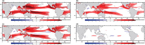
Next, we investigate the impact of changing sample members on the projected change in GPI. The projected change in GPI for the late–21st-century A2 scenario is calculated for E-II, E-III and E-IV and the results are shown in Fig. 5. Black contours show where the change in GPI for E-II, E-III, E-IV and E-V are significantly different from E-I. The projected changes show spatial patterns that are qualitatively similar to each other; however, the magnitudes are different in each ocean basin, consistent with the results shown in Fig. 4. As for the current climate, the choice of the sample models for the late–21st-century climate also impacts the resultant projections of GPI change.

In comparison with E-I, the projected change in GPI for E-II shows a large and extensive increase in the GPI in the Central Pacific (Fig. 5a) and a projected decrease in GPI to the North and West of Australia. The projected change in E-II for North Western Australia is now of opposite sign to that calculated in E-I. The projected change in GPI calculated for E-III is similar to that from E-II but produces smaller decreases in GPI change for the North Atlantic. The pattern of GPI change for E-IV differs from that for E-III but is similar to E-I in most regions except the North West Pacific in the region close to Japan and the Philippines and in North West Australia. The magnitude of projected change in GPI for the North West and North Central Pacific is lower in E-IV compared with both E-II and E-III.

Fig. 5.  Change in mean GPI between late–21st- and 20th-century climate (a) E-II, (b) E-III, (c) E-IV and (d) E-V. Contours show values which are 95% significantly different from E-I.

The purpose of Ensemble E-V was to investigate the impact of subsampling the models in E-I which belong to the same family. In other words, the models from the same family are identified in E-I and are: CSIRO-Mk3.0 and 3.5, GFDL-CM2.0 and 2.1 and UK.HadCM3 and UK.HadGEM1. An examination of the GPI changes (Fig. 2) for each of these models showed that there is a marked similarity between the projected patterns of change for models from the same family. The analysis of Masson and Knutti (2011) indicates that these models are similar to each other and cluster together. Hence, the change in GPI between the late–20th- and 21st-century climates is calculated using the mean change in GPI for the GFDL, CSIRO and UK Hadley Centre families of models. Based on naming, INGV-ECHAM4 and MPI ECHAM5 appear to be from the same family; however, the analysis of Masson and Knutti (2011) identified considerable differences between the models, and so they are considered to be independent samples for this case. The projected pattern and magnitude of change in GPI for ensemble E-V is very similar to that of E-I.

It can therefore be inferred from the results of Fig. 5 that the projected ensemble mean change in the GPI for the future climate scenario is dependent upon the sample of models chosen to make up the current and future climate ensembles. Thus, the choice of the models in an ensemble is very important in determining the result. It has the capacity to generate results which might contradict each other if not undertaken cautiously.

It has previously been noted (Fig. 2) that the change in GPI shows considerable variability between models. Some models, for instance IPSL-CM4 and MRI-CGCM2, show strong overall positive change in GPI for late–21st-century, whereas MIROC-medres, GISS_E_R and INGV-ECHAM4 show an overall decrease. Thus, the difference in the median of GPI may be the best indicator of the projected change in GPI for each ensemble. Results based on the median are shown in Fig. 6.

Fig. 6.  Change in median GPI between late–21st- and 20th-century climate (a) E-I, (b) E-II, (c) E-III, (d) E-IV and (e) E-V.

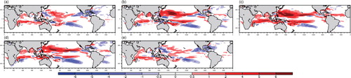
The results shown in Fig. 6 are similar in their overall features compared with the mean change shown in Fig. 5. The median change in GPI for late–21st-century climate for ensemble E-I and E-V are very similar; however, E-I shows a larger region of increase in GPI in the North Central Pacific compared with E-V. Hence, in this case, the median change in the GPI does not show significant differences when models belonging to the same family are considered to have a single realisation. In some regions, such as the North West Pacific near Japan and the North East Pacific, the signs of projected changes vary from E-I (paired samples) to E-II (unpaired samples), highlighting the importance of using paired samples in analysis. The median patterns of change in the GPI for all ensembles are similar to the patterns of change in the mean, although the magnitudes differ. Ensembles E-II, E-III and E-IV show the largest projected increase in GPI in the Northern Hemisphere. All ensembles show a decrease in the median GPI for the Central South Pacific. The main differences between the two methods occur in the region off North-Western Australia. In this region, the median pattern of change is for little change to increases in GPI for the late–21st-century, while the mean pattern of change shows results ranging from a decrease in GPI (EI and EII) to an increase in GPI.

It can therefore be concluded from these results that the projected change in the GPI is sensitive to the choice of models used to define the late–20th-century and the late–21st-century mean climates. After ensuring that paired samples were used for both current and future climates, our results show that the projected change in GPI is for a moderate increase over the Central North Pacific, North Indian and South Indian basins and a decrease over the North Atlantic, North East Pacific, North West Pacific and South Pacific basins.

4. Conclusion

The GPI of Emanuel and Nolan (2004) was applied to 16 GCMs from the CMIP3 models to study their ability to infer TC genesis in the current climate and to identify the change in GPI in a future climate based on the IPCC SRES A2 scenario. It was found that although the models were successful in simulating the TC genesis area when compared against NCEP and ERA40 reanalysis data, most of the models underestimated the magnitude of the GPI compared with that calculated from the ERA40 reanalysis and showed similar magnitudes to that calculated from the NCEP reanalysis.

The change in the GPI for the late–21st-century based on IPCC SRES A2 scenario was also calculated. The models showed considerable variability in their climate change response to the differences in GPI, especially over the Central Pacific and the South Pacific basins. The ensemble mean from all models showed moderate increase over the Central North Pacific, North Indian and South Indian basins and a decrease over the North Atlantic, North East Pacific, North West Pacific and South Pacific basins.

The focus of this study has been to investigate the impact of sampling on the development of projections for changes in tropical cyclogenesis as inferred through the GPI. Since there is considerable inter-model variability in the climate change response to the GPI, the models selected have the potential to be extremely important in the development of these projections. Thus, five ensembles were considered with the composition of the ensembles designed to investigate the use of paired versus unpaired samples and the impact of using multiple models from the same family.

When the GPI analysis was repeated using different ensemble members, the magnitude of the change was found to vary significantly. Ensemble E-II (based on Caron and Jones, 2008) used multiple realisations from five models for its late–20th-century climate; however, its 21st-century climate did not have representation for two models and had multiple realisations for two other models; hence, E-II has 18 models for its late–20th-century climate and 9 models for its 21st-century climate. The projected change in GPI for E-II shows a large and extensive increase in the GPI in the Central Pacific (Fig. 5a) and a projected decrease in GPI to the North and West of Australia. Importantly, the projected change in E-II for some regions is now of opposite sign to that calculated in E-I. These changes, using unpaired samples, are significantly different from those of E-I which used paired samples.

Ensembles E-III and E-IV use the models of E-II but transition towards paired samples. Ensemble E-III uses the same models as E-II for both the late–20th and 21st-century climate, but a mean GPI is calculated for the models with multiple realisations. Hence, E-III has nine models for the late–20th-century climate and seven models for the late–21st-century climate. The projected change in GPI calculated for E-III is similar to that from E-II but produces smaller decreases in GPI change for the North Atlantic which are shown in Fig. 5b.

Ensemble E-IV is similar to E-III; however, the models that do not have a representation in the 21st-century climate have been eliminated from the 20th-century climate calculations. It has paired samples of seven models in both late–20th- and 21st-century climates. Although E-IV has paired samples, the number of samples are less than half compared with E-I. The pattern of GPI change for E-IV differs from that for E-III but is similar to E-I in most regions as shown in Fig. 5c.

Ensemble E-V consists of the same models as E-I, but a mean GPI is calculated for the models belonging to the same family. E-V has paired samples of 13 models in its late–20th- and 21st-century climate. The magnitude of projected change in GPI for the North West and North Central Pacific is lower in E-IV compared with both E-II and E-III. E-V is not significantly different to E-I.

We therefore conclude that it may not be desirable to calculate the mean of a model ensemble when a subset of models has more than one realisation compared with the others. This process over-emphasises the features of a particular model with more realisations over that of the others. It is therefore essential to select individual members of an ensemble cautiously as this has the capacity to alter the results.

After ensuring that paired samples were used for both current and future climates, our results show that the projected changes in GPI are for an increase in GPI over the Central North Pacific, North Indian and South Indian basins and a decrease over the North Atlantic, North East Pacific, North West Pacific and South Pacific basins.

Acknowledgements

The research discussed in this article was conducted with the support of Pacific Climate Change Science Program, a programme supported by AusAID, in collaboration with the Department of Climate Change and Energy Efficiency and delivered by the Bureau of Meteorology and Commonwealth Scientific and Industrial Research Organisation (CSIRO). We acknowledge the modelling groups, the Program for Climate Model Diagnosis and Inter-comparison (PCMDI) and World Climate Research Programme's (WCRP) Working Group on Coupled Modelling for their roles in making available the WCRP CMIP3 multimodel dataset. More details on the model documentation are available at the PCMDI website (http://www-pcmdi.llnl.gov). I acknowledge Dr Sally Lavender and Dr Marcus Thatcher for providing me with the codes and scripts along with Dr Penny Whetton, Dr Will Thurston, Dr Fabrice Chauvin and two anonymous reviewers for providing me with comments which improved the article immensely. Fabrice Chauvin also kindly provided plots of his projected changes for comparison with our calculations.

References

- Biasutti, M and Giannini, A. 2006. Robust Sahel drying in response to late 20th century forcings. Geophys. Res. Lett. 33, L11706. 10.3402/tellusa.v64i0.18696.
- Bister M. Emanuel K. A. Dissipative heating and hurricane intensity. Meteorol. Atmos. Phys. 1998; 50: 233–240. 10.3402/tellusa.v64i0.18696.
- Bony S. Sud Y. Lau K. M. Susskind J. Saha S. Comparison and satellite assessment of NASA/DAO and NCEP-NCAR reanalyses over tropical ocean: atmospheric hydrology and radiation. J. Clim. 1997; 10: 1441–1461. 10.3402/tellusa.v64i0.18696.
- Camargo S. J. Emanuel K. A. Sobel A. H. Use of Genesis Potential Index to diagnose ENSO effects on tropical cyclone genesis. J. Clim. 2007a; 20: 4819–4834. 10.3402/tellusa.v64i0.18696.
- Camargo S. J. Sobel A. H. Barnston A. G. Emanuel K. A. Tropical cyclone Genesis Potential Index in climate models. Tellus. 2007b; 59A: 428–443.
- Caron L.-P. Jones C. G. Analysing present, past and future tropical cyclone activity as inferred from an ensemble of Coupled Global Climate Models. Tellus. 2008; 60A: 80–96.
- Chauvin, F and Royer, J.-F. 2010. Role of SST anomaly structures in response of cyclogenesis to global warming. In: Hurricanes and Climate Change. J. B. Elsner, R. E. Hodges, J. C. Malmstadt and K. N. ScheitlinVol. 2, pp. 39–56. Springer Science+Business Media B.V. 2010, DOI: 10.1007/978-90-481-9510-7_3.
- Chauvin F. Royer J.-F. D′equ′e M. Response of hurricane type vortices to global warming as simulated by ARPEGE-climate at high resolution. Clim. Dyn. 2006; 27: 377–399. 10.3402/tellusa.v64i0.18696.
- Delworth, T. L, Brocoli, A. J, Rosati, A, Stouffer, R. J, Balaji, V and co-authors. 2006. GFDL's CM2 global coupled climate models. Part 1: formulation and simulation characteristics. J. Clim. 9, 643–674. 10.3402/tellusa.v64i0.18696.
- Dessler A. E. Davis S. M. Trends in tropospheric humidity from reanalysis systems. Geophys. Res. Lett. 2010; 115: D19127.
- Emanuel K. Sensitivity of tropical cyclones to surface exchange coefficients and a revised steady-state model incorporating eye dynamics. J. Atmos. Sci. 1995; 52: 3969–3976. 10.3402/tellusa.v64i0.18696.
- Emanuel K. Increasing destructiveness of TCs over the past 30 years. Nature. 2005; 436: 686–688. 10.3402/tellusa.v64i0.18696.
- Emanuel K. Sundararajan R. Williams J. Hurricanes and global warming: results from downscaling CMIP3 simulations. Bull. Am. Meteorol. Soc. 2008; 89: 347–367. 10.3402/tellusa.v64i0.18696.
- Emanuel, K. A and Nolan, D. S. 2004. Tropical cyclone activity and global climate. In: Proceedings of 26th Conference on Hurricanes and Tropical Meteorology, Miami, Florida, American Met. Soc. 240–241.
- Flato, G. M, Boer, G. J, Lee, W. G, McFarlane, N. A, Ramsden, D, Reader, M. C and Weaver, A. J. 2000. The Canadian Centre for Climate Modeling and Analysis Global Coupled Model and its Climate. Climate Dynamics. 16, 451–467. 10.3402/tellusa.v64i0.18696.
- Furevik T. Bentsen M. Drange H. Kvamsto N. Sorteberg A. Description and evaluation of the Bergen climate model: ARPEGE coupled with MICOM. Clim. Dyn. 2003; 21: 27–51. 10.3402/tellusa.v64i0.18696.
- Galin, V. Ya, Volodin, E. M and Smyshliaev, S. P. 2003. Atmosphere general circulation model of INM RAS with ozone dynamics. Russ. Meteorol. Hydrol. N5, 13–22.
- Gordon, H. B, Rotstayn, L. D, McGregor, J. L, Dix, M. R and Kowalczyk, E. A. 2002. The CSIROMk3 Climate System Model. Technical Report 60, CSIRO Atmospheric Research, Aspendale.
- Gray, W. M. 1979. Hurricanes: their formation structure and likely role in tropical circulation. In: Meteorology Over the Tropical Oceans. D. B. Shaw, Royal Meteorological Society, James Glaisher House, Grenville Place, Bracknell, Berkshire, RG12 1BX, pp. 155–218.
- Holland, G and Webster, P. J. 2007. Heightened tropical cyclone activity in the North Atlantic: natural variability or climate trend? Weather and Climate Extremes in a Changing Climate, National Climatic Data Center. Online at: http://www.climatescience.gov/Library/sap/sap3-3/finalreport/default.htm.
- Johns, T, Durman, C, Banks, H, Roberts, M, McLaren, A and co-authors. 2004. HadGEM1 – Model Description and Analysis of Preliminary Experiments for the IPCC Fourth Assessment Report. Technical Report 55, UK Met Office, Exeter, UK.
- K-1 Model developers. 2004. K-1 Couple Model (MIROC) Description. Technical Report 1, Center for Climate System Research, University of Tokyo, Tokyo.
- Knutson, T. R, McBride, J. L, Chan, J, Emanuel, K, Holland, G and co-authors. 2010. Tropical cyclones and climate change. 3, 157–163. 10.3402/tellusa.v64i0.18696.
- Landsea C. W. Counting Atlantic cyclones back to 1900. Nat. Geosci. 2007; 18: 197–202. 10.3402/tellusa.v64i0.18696.
- Marti, O, Braconnot, P, Bellier, J, Benshila, R, Bony, S and co-authors. 2005. The New IPSL Climate System Model: IPSLCM4. Technical Report, Institut Pierre Simon Laplace des Sciences de l'Environnement Global, IPSL, Case 101, 4 place Jussieu, Paris, France.
- Masson D. Knutti R. Climate model genealogy. 2011; 38: L08703.10.3402/tellusa.v64i0.18696.
- Menkes, C. E, Lengaigne, M, Marchesiello, P, Jourdain, N. C, Vincent, E. M and co-authors. 2012. Comparison of tropical cyclogenesis indices on seasonal to interannual timescales. Geophys. Res. Lett. 38, 301–321. 10.3402/tellusa.v64i0.18696.
- Peterson, T. C, Anderson, D. M, Cohen, S. J, Cortez-Vázquez, M, Murnane, R. J and co-authors. 2008. Why weather and climate extremes matter. In: Weather and Climate Extremes in a Changing Climate. Regions of Focus: North America, Hawaii, Caribbean, and U.S. Pacific Islands. T. R. Karl, G. A. Meehl, C. D. Miller, S. J. Hassol, A. M. Waple and W. L. Murray. A Report by the U.S. Climate Change Science Program and the Subcommittee on Global Change Research, Washington, DC.
- Roeckner, E, Bäuml, G, Bonaventura, L, Brokopf, R, Esch, M and co-authors. 2003. The Atmospheric General Circulation Model ECHAM5. Part 1: Model Description. Max-Planck-Institut für Meteorologie, Report 349, 127 pp.
- Royer J.-F. Chauvin F. Timbal B. Araspin P. Grimal D. A GCM study of the impact of greenhouse gas increase on the frequency of occurrence of tropical cyclones. 1998; 38: 307–343. 10.3402/tellusa.v64i0.18696.
- Ryan B. F. Watterson I. G. Evans J. L. Tropical cyclone frequencies inferred from Gray's yearly genesis parameter: validation of GCM tropical climates. Clim. Change. 1992; 19: 1831–1834. 10.3402/tellusa.v64i0.18696.
- Schmidt, G. A, Ruedy, R, Hansen, J. E, Aleinov, I, Bell, N and co-authors. 2006. Present day atmospheric simulations using GISS Model E: comparison to in-situ, satellite and reanalysis data. Geophys. Res Lett. 19, 153–192. 10.3402/tellusa.v64i0.18696.
- Salas-Melia, D, Chauvin, F, Deque, M, Douville, H, Gueremy, J and co-authors. 2005. Description and validation of the CNRM-CM3 global coupled model. CNRM, Note de Centre number 103, http://www.cnrm.meteo.fr/scenario2004/paper_cm3.pdf.
- Trenberth, K. E and Shea, D. J. 2006. Atlantic hurricanes and natural variability in 2005. 33, L12704. 10.3402/tellusa.v64i0.18696.
- Villarini G. Vecchi G. A. Knutson T. R. Zhao M. Smith J. A. North Atlantic tropical storm frequency response to anthropogenic forcing: projections and sources of uncertainty. Geophys. Res. Lett. 2011; 24: 3224–3239. 10.3402/tellusa.v64i0.18696.
- Vecchi, G. A and Soden, B. J. 2007. Increased tropical cyclone wind shear in model projections of global warming. J. Clim. 34, L08702. 10.3402/tellusa.v64i0.18696.
- Watterson I. G. Evans J. L. Ryan B. F. Seasonal and interannual variability of tropical cyclogenesis: diagnostics from large-scale fields. Geophys. Res. Lett. 1995; 8: 3052–3066. 10.3402/tellusa.v64i0.18696.
- Webster P. J. Holland G. J. Curry J. A. Chang H. R. Changes in TC number, duration and intensity in a warming environment. 2005; 309(5742): 1844–1846. 10.3402/tellusa.v64i0.18696.
- Yokoi S. Takayabu Y. N. Chan J. C. L. Tropical cyclone genesis frequency over the western North Pacific simulated in medium resolution coupled GCM. J. Clim. 2009; 33: 33665–33683. 10.3402/tellusa.v64i0.18696.
- Yukimoto, S and Noda, A. 2003. Improvements of the Meteorological Research Institute Global Ocean-atmosphere Coupled GCM (MRICGCM2) and Its Climate Sensitivity. Technical Report 10, National Institute for Environmental Studies, Japan.
- Zhang Y. Wang H. Sun J. Drange H. Changes in tropical cyclone Genesis Potential Index over the Western North Pacific in the SRES A2 scenario. Clim. Dyn. 2010; 27(6): 1246–1258. 10.3402/tellusa.v64i0.18696.