Assimilation of low-level wind in a high-resolution mesoscale model using the back and forth nudging algorithm

ABSTRACT

The performance of a new data assimilation algorithm called back and forth nudging (BFN) is evaluated using a high-resolution numerical mesoscale model and simulated wind observations in the boundary layer. This new algorithm, of interest for the assimilation of high-frequency observations provided by ground-based active remote-sensing instruments, is straightforward to implement in a realistic atmospheric model. The convergence towards a steady-state profile can be achieved after five iterations of the BFN algorithm, and the algorithm provides an improved solution with respect to direct nudging. It is shown that the contribution of the nudging term does not dominate over other model physical and dynamical tendencies. Moreover, by running backward integrations with an adiabatic version of the model, the nudging coefficients do not need to be increased in order to stabilise the numerical equations. The ability of BFN to produce model changes upstream from the observations, in a similar way to 4-D-Var assimilation systems, is demonstrated. The capacity of the model to adjust to rapid changes in wind direction with the BFN is a first encouraging step, for example, to improve the detection and prediction of low-level wind shear phenomena through high-resolution mesoscale modelling over airports.

• Data assimilation
• Nudging
• Low-level wind

1. Introduction

Recent progress in mesoscale data assimilation has been such that a number of weather centres run operationally convective scale numerical models with grid mesh less than 5 km (e.g. COSMO consortium, UK MetOffice, Météo-France). These models are initialised by assimilating both conventional and satellite observations, together with dedicated data such as radial Doppler winds (Montmerle and Faccani, 2009), radar reflectivities (Caumont et al., 2010) or wind profiles from vertically pointing Ultra High Frequency/Very High Frequency (UHF/VHF) radars. However, the potential of these mesoscale data is not yet fully exploited. For example, their spatial and temporal distributions are thinned to avoid correlated observations and spin-up problems. Radar reflectivity innovations are converted into humidity profiles or diabatic heating rate profiles before assimilation. Wind observations from UHF radars are often not assimilated in the boundary layer due to large discrepancies between measurements and model counterparts. The increase in resolution of mesoscale models below 1 km and the availability of new types of ground-based active instruments with high temporal sampling capabilities (microwave radiometers, water vapour and wind lidars and cloud and wind radars) present new challenges for data assimilation. Indeed, detection and forecast of weather hazards (wind shears, wind bursts and fog events) over sensitive areas such as airport runways could be improved using such high-resolution numerical systems, with obvious consequences in terms of security and economy. The present study describes a preliminary investigation in this area by assimilating, at a high-frequency, low-level simulated UHF wind profiler observations into a subkilometric mesoscale model.

Three main assimilation techniques are currently used for operational mesoscale prediction models: three-dimensional variational (3-D-Var), four-dimensional variational (4-D-Var) systems and nudging. The ensemble Kalman filter is a promising data assimilation system that is used operationally with global models (e.g. Houtekamer et al., 2005). This method is still under development for the mesoscale but provides encouraging results with pre-operational systems (e.g. Bonavita et al., 2010; Torn and Hakim, 2008). In 3-D-Var systems, the time dimension of observations is not accounted for. However, the Increment Analysis Update (IAU; Bloom et al., 1996) method incorporates analysis increments as a continuous forcing over a period of time, but these increments need to be computed first by a data assimilation system. Four-dimensional variational systems provide an analysis consistent with the model dynamics and all observations over a given time window. Nevertheless, the required linearisation of physical processes can be questionable at subkilometre scale (e.g. cloud microphysics). Nudging schemes are simpler to develop but rely on empirical coefficients that are more difficult to optimally define for a particular situation than background error covariance matrices (Zou et al., 1992). An advantage of the nudging over 3-D-Var is that it accounts for model dynamics in order to fit observations. Recently, Auroux and Blum (2005) proposed a new nudging technique: back and forth nudging (BFN). It consists of iterative model adjustments towards the observations through a series of forward and backward nudging integrations. Such a BFN method could be applied to IAU, but it would require an assimilation system (e.g. 3-D-Var) to compute the analysis increments. The BFN algorithm aims at determining an optimal initial condition by considering all available data over a time window as is done by a 4-D-Var. Indeed, Auroux and Blum (2008) found the BFN compared favourably against 4-D-Var with simple models (Lorenz model, Burgers equations, shallow water model). One objective of our study is to examine the BFN with a more realistic numerical model: the atmospheric mesoscale model Meso-NH (Lafore et al., 1998). In this preliminary investigation, only simulated observations are considered in order to control the solution where the BFN should converge. We chose low-level wind observations to restrict the relevant physical processes to turbulence in the planetary boundary layer. Moreover, a number of numerical simulations with Meso-NH at 500 m resolution have shown that this model has some skill in forecasting low-level wind shear events, although not necessarily at the proper location or the correct time (Bidet and Schwartz, 2006; Boilley et al., 2008). In a future study, we plan to examine how the assimilation of wind profiler data could allow Meso-NH to better predict these weather hazards. In Section 2, the mesoscale model is presented together with the BFN technique. Section 3 describes the experimental design. Results from data assimilation and sensitivity experiments are shown in Section 4. In particular, the BFN is compared with the standard nudging technique. Conclusions and perspectives from this study are provided in Section 5.

2. Model and BFN algorithm

2.1. Description of the model

The numerical simulations are performed with the non-hydrostatic Meso-NH model (Lafore et al., 1998) which is based on the anelastic approximation with purely explicit second-order accurate spatial and temporal discretisations. The prognostic variables are the three wind components, dry potential temperature, the mixing ratio of six different classes of water and turbulent kinetic energy. The model contains a comprehensive set of physical parameterisation schemes to describe subgrid scale processes. In particular, the turbulent flux computations use the Cuxart et al. (2000) method, and can either be purely vertical or fully 3-D. In the former case, the mixing length is given by the Bougeault and Lacarrère (1989) formulation and in the latter case by Deardorff (1972).

2.2. BFN algorithm

The BFN algorithm introduced by Auroux and Blum (2005) consists of repeatedly performing forward and backward integrations of the model with relaxation (or nudging) terms, using opposite signs in direct and inverse integrations, so as to make the backward evolution numerically stable. The aim of the nudging term is to assimilate data by constraining the model dynamical tendencies to draw towards observations. After each iteration (which consists of a forward integration followed by a backward integration), an estimate of the initial condition of the system is obtained. The forward and backward integrations (with the relaxation terms) are repeated until convergence is reached. This method allows the model to find a trajectory over a given time window that is both consistent with the dynamics and the available observations. We refer to Auroux and Blum (2008) for further details of the algorithm. The Meso-NH equations for each prognostic variable X have been modified to take into account the nudging towards available observations, Y _o:1

where F represents the dynamical and physical model tendencies. The second term on the right-hand side is the nudging term; the summation is over all observations. The nudging time constant, τ, determines the rate at which the model variable converges towards observations. The observation operator, H, gives the model equivalent of the observations (in our study, H is a simple spatial interpolation scheme). Details about the spatial and temporal weighting function, W, that spreads the observation departure [H(X) − Y _o] back to the model space are given in the next section. Nielsen-Gammon et al. (2007) reported that ‘observation nudging’ is appropriate when high-frequency observations are available or when the analysis cannot resolve important features in the model simulation. They also mention that the particular form of the nudging weight (square value in the numerator) suggested by Benjamin and Seaman (1985) reduces the strength of the nudging when multiple observations affect a given model point.

The backward nudging consists of integrating the model equations backward in time starting from the state obtained at the end of the forward model integration. The backward equations of the model state with a nudging term can be written:2

The relaxation constant, τ′, and the weighting function, W′, can be different from values specified in the forward integration. Indeed, Auroux and Blum (2008) recommend using a τ′ smaller than τ in order to stabilise the backward integration when irreversible (dissipative) processes are present in the model equations.

3. Experimental design

The objective of this study is to examine the suitability of the BFN algorithm for a high-resolution numerical atmospheric mesoscale model and high temporal frequency observations, knowing that direct nudging schemes are currently tested in that context (COSMO consortium; Hug et al., 2010).

3.1. Domain and initial conditions

The initial conditions for the assimilation experiment are obtained after 4 h of simulation in the following configuration. The experimental domain has been defined over flat terrain without heat and water exchanges between the surface and the atmosphere. The horizontal resolution is 500 m with 40 grid points in each direction. The domain size was chosen large enough to avoid increments reaching boundaries over the assimilation window. The vertical resolution varies with height from 10 m above the ground to 800 m in the stratosphere, with 60 levels in total. The top of the model is at an altitude of 14 km. The resolution in the boundary layer is such that 32 levels are located below 2 km. The model time step has been set to 6 s. The initial conditions are horizontally homogeneous, the horizontal wind has a zonal direction and an intensity of 1 m s⁻¹ with a reduction in the boundary layer using a log-shaped profile. The potential temperature is set equal to the surface temperature (281 K) below 1 km (neutral stability) with a stable profile in the troposphere. The water vapour mixing ratio is set to zero and moist physical processes are not activated in the model. The normal velocity component at the lateral boundaries is computed using a wave-radiation open boundary condition proposed by Carpenter (1982) with a phase speed value set to the normal velocity. The tangential velocity and all the other prognostic variables are extrapolated from the interior at outflow conditions. Similarly, inflow conditions are specified at the boundary from large-scale values. Given the small size of the domain and the need to reach a stationary solution when no data are assimilated, the effect of the Earth's rotation has been neglected. The vertical diffusion scheme is the only physical process activated in the model, and it uses the Bougeault and Lacarrère (1989) mixing length formulation. This choice is justified by the experimental design (observations in the lower troposphere and a short temporal assimilation window). This simplified model configuration allows to start an examination of the influence of (dissipative) physical processes on the BFN algorithm, without the full complexity of other parameterisation schemes available in Meso-NH.

3.2. Data assimilation experiments

Backward integrations of atmospheric models have already been performed in the context of digital filtering initialisation (Lynch and Huang, 1992) and data assimilation [quasi-inverse algorithm proposed by Kalnay et al. (2000)]. In order to avoid computational blow-up, the model can either be run adiabatically or the sign of the dissipative terms can be changed. The solution proposed by Auroux and Blum (2005) is to keep the model equations unchanged, but to increase the weight of the nudging term in the forcing tendencies [i.e. the factor τ′ defined in eq. (2) should be much smaller than τ defined in eq. (1)]. The current implementation of the BFN algorithm in Meso-NH is such that in the backward integration all physical processes are switched off. This approach allows the use of the same time constant τ in the direct and retrograde integrations of the model. This choice has some similarities with the incremental approach of variational data assimilation (Courtier et al., 1994) which solves the minimisation with a simplified linearised numerical model.

The weight W _xyzt of the nudging coefficient defined in eq. (3) allows the influence of a given observation to be distributed in space and time. It has the same role as the gain matrix in Kalman filters and variational assimilations. It is a function of the difference in 3-D space and time between the observation location and the grid point location, and is expressed as the product of a horizontal weight W _xy, a vertical weight W _z and a temporal weight W _t:3

The horizontal weight is defined as a function of the distance d between an observation and a model grid point with a scale radius R _xy following an exponential correlation model:4

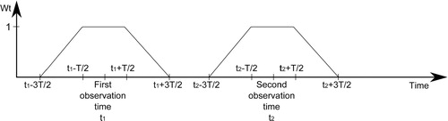
The same model as eq. 4 is used for the vertical weight, with a scale radius R _z. The temporal weight W _t is defined as a function of a time window half-width T. The weight is defined as 1 when the model is within T/2 of the observation time, 0 when it is beyond 1.5 × T of the observation time and a linear transition from 0 to 1 (or 1 to 0) when the model is between –1.5 × T and –0.5 × T (or 0.5 × T and 1.5T) of the observation time (Fig. 1).

Fig. 1.  Evolution of the temporal weight W _t for two consecutive observations.

We have considered the assimilation of simulated horizontal wind observations over an assimilation window of 1 h. In order to mimic the vertical extent of data from a UHF wind profiler, we have assumed that observations are provided from 100 to 3000 m above the surface, with a temporal availability of 10 min. In a first set of experiments, a single profile located at the centre of the domain with a constant direction (zonal wind) and intensity of 2 m s⁻¹ (except near the surface) is considered. These experiments have been carried out to examine the convergence of the BFN and its sensitivity to the various tunable input parameters. In a second set of experiments, a steady wind rotation is assimilated to demonstrate the capacity of the BFN algorithm to improve the model simulation of wind shear events.

Typical values of τ vary between 1000 and 10 000 s (Stauffer and Seaman, 1990). Stauffer and Seaman (1990) argue that τ should be similar in magnitude to the slowest adjustment time scale of the relevant forcing tendencies F. In the present experimental set-up, it has been set to 1000 s. Similarly, the scale radius is set to R _xy=1500 m on the horizontal and to R _z=100 m on the vertical. The sensitivity of the results to these specifications is assessed below.

4. Numerical results

4.1. Observations with a constant wind

We first study the numerical convergence of the BFN algorithm towards a simulated observation wind profile with a westerly direction (i.e. u _obs=2 m s⁻¹ and v _obs=0 m s⁻¹) located at the centre of the experimental domain. Observations are provided at each model level between 100 and 3000  m. We consider observations extracted at the end of a reference 4-h simulation (considered as the truth) initialised with a constant value of 2 m s⁻¹ above 1000 m, values decreasing towards 0 at the roughness length level (z ₀=1 cm), following a log-shape profile. The vertical model resolution is around 25 m below 500 m, which compares well with the vertical resolution of a UHF wind profiler (around 35 m). Above 500 m the vertical model resolution becomes coarser with values around 200 m at 3000  m. The assimilation window is set to 1 h and the temporal weight W _t is set to 1 (the model is continuously forced towards the same observation profile), to examine the behaviour of the BFN in a stationary regime (as if the same wind profile was observed at each time step). The horizontal size of the computational domain, the location of the observed wind profile in the middle of the domain and its intensity, together with the assimilation time window, have been chosen such that the lateral boundary conditions do not affect the behaviour of the nudging scheme.

4.1.1. Convergence of the BFN.

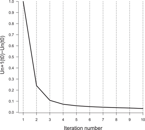
Figure 2 shows the evolution of the mean absolute difference between the zonal wind fields of two consecutives iterations, for all the vertical levels concerned by the nudging and all the horizontal grid points, for 10 BFN iterations. It shows that during the five first iterations of the BFN, the difference with the previous state is reduced by more than 90% while the five following iterations only induce a gain of 2.5%. For that reason the following experiments are limited to five BFN iterations. Since the gain is limited from the fifth iteration to the tenth, this set of iterations defines the stationary regime of the BFN method.

Fig. 2.  Evolution of the mean absolute difference between the zonal wind fields of two consecutive iterations, for all the vertical levels influenced by the nudging and all the horizontal grid points, for 10 BFN iterations.

We then define a global measure for the BFN convergence that is a weighted root mean square error [RMSE(t)] using the horizontal weight W _xy of the nudging coefficient:5

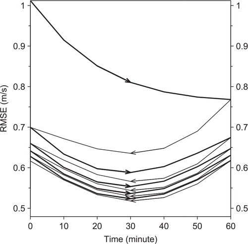
where the summation is over all model grid points on the horizontal and over all vertical levels between 100 and 3000 m. This formulation gives a stronger weight to grid points located close to the observations, as they are most influenced by the nudging. Figure 3 shows the evolution of the RMSE(t) over the assimilation window for five iterations of the BFN. After one iteration, the direct nudging has decreased the error by 0.23 m s⁻¹, with a fast decrease during the first half of the period and a slower reduction afterwards. The backward nudging contributes to a further decrease of the error by 0.07 m s⁻¹. The following iterations continue to reduce the value of RMSE(t) but at a slower rate. After five iterations of the BFN, the initial error has been reduced by 40%. Auroux (2008) reported a similar convergence rate in a shallow water model forced with perfect observations. It is encouraging that the backward integration significantly reduces the error remaining after each direct nudging integration, and that the subsequent direct model integrations also generate a more accurate solution. Except for the first direct integration, the error minimum is obtained in the middle of the assimilation window. This behaviour is consistent with a strong constraint variational assimilation, where the closest fit of a model solution to observations is found at the mid-point of the assimilation window, and the farthest fit occurs at the start and finish of the window (Talagrand, 1999).

Fig. 3.  RMSE between BFN iterations (five iterations) and the true wind profile over the assimilation window (constant wind observation). Each thick solid line represents a direct nudging integration and each thin solid line represents a retrograde nudging integration.

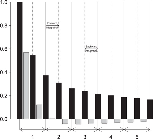
The error reduction in the zonal wind is examined further at the observation point for an arbitrary altitude (2000 m) above the boundary layer (Fig. 4). This diagram shows the difference at the beginning and end of each assimilation window (black bars), and also in the middle (grey bars). One would expect the best fit to observations for that particular location due to small turbulence effects above the boundary layer and to the horizontal scale radius centred on the observation location. This is indeed the case in that the initial error of 1 m s⁻¹ is reduced to 0.38 m s⁻¹ after one BFN iteration (i.e. one forward integration followed by a backward integration). Each iteration brings a further reduction of the error. Almost no changes can be noticed by the last iteration (small reduction of 0.01 m s⁻¹), showing that the algorithm has converged at that particular location. When examining the error in the middle of the time window, it appears that the model has reached the observed value of 2 m s⁻¹ after the second iteration. At the next iteration, the model slightly overshoots the observation by 0.05 m s⁻¹ since the error has changed sign. Then, the error is slightly reduced by the subsequent iterations. The overshooting of the model at the observed location (Fig. 4) allows the surrounding points to better fit the observation, as shown in the evolution of the global RMSE(t).

Fig. 4.  Observed minus modelled zonal wind at observation location during the BFN iterations (at an altitude of 2000 m). Black bars correspond to values at both ends of the assimilation window, and grey bars correspond to values at the middle of the assimilation window. Vertical lines allow to distinguish between forward and backward model integrations.

The effect on potential temperature of wind assimilation is negligible. The maximum difference in potential temperature field between initial time and after 10 iterations is about 2.10⁻² degrees.

4.1.2. Sensitivity to the nudging time scale.

In order to examine the contribution of the nudging term to the dynamical model tendencies, the budget terms for the momentum equations have been computed at each model level, and integrated temporally every minute (10 model time steps):

The subscripts ‘advx’, ‘advy’, ‘pres’, ‘turb’ and ‘nudg’ correspond, respectively, to the contributions of advection along x, advection along y, pressure gradient, vertical turbulent diffusion and nudging. The overline operator represents the spatial and temporal averages of the tendencies. Other budget terms are not examined here because they represent a negligible contribution to the total tendencies. The budget terms are examined for three values of the nudging time scale τ, 500, 1000 and 2500 s, at two particular model levels within and above the boundary layer (150 and 2000 m). To examine the magnitude of the individual terms, their absolute values are shown in Fig. 5 for five iterations of the BFN. For all values of τ, except at the beginning of the first iteration, the nudging term is rather small compared with the advection and pressure terms. A rapid mass adjustment to wind changes imposed by the nudging can be seen on the pressure term at the beginning of the first iteration. The large initial contribution of the pressure term which counterbalances the nudging term decreases when τ increases. With a value of τ=500 s, a stationary solution is obtained at the end of the first BFN iteration, whereas with τ=2500 s after five BFN iterations an increase of the advection terms can still be noticed. As shown previously in Fig. 3, with τ=1000 s the stationary regime (defined in Section 4.1.1) is reached after four BFN iterations. The rather large value of the pressure gradient at the beginning of each model integration highlights a model imbalance between the wind and mass fields. This is the result of the method used to integrate the model Meso-NH backwards. Instead of setting the model time step to a negative value, the wind components are inverted. Since the temperature and pressure fields are not modified accordingly, an initial adjustment process takes place during the first 2 min of each model integration. The fluctuations of the pressure gradient tendencies during the first model time steps are about 10% of the actual values (Fig. 5). Temperature and wind output fields examined after 10 min of model integration (not shown) did not reveal any sign of imbalance (such as noise or gravity waves). The strength of this imbalance is indeed related to the value of the nudging time constant. If the imbalance could be an issue (e.g. for less idealised meteorological situations), a solution would be to increase the time constant τ. Another option would be to revise the strategy for the backward integration of the model.

Fig. 5.  Evolution of the budget terms (absolute values) from the zonal wind dynamical equations at two model levels (top row = 150 m and bottom row = 2000 m) for three values of the nudging time constant τ (left column = 500 s, middle column = 1000 s and right column = 2500 s). The horizontal axis represents the time over the ten 1-h model integrations (five direct runs and five retrograde runs in alternance). The existence of discontinuities for the turbulence term is the consequence of adiabatic backward integrations ofMeso-NH.

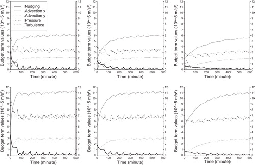
The above results show that regardless of the value of τ (between 500 and 2500 s), the nudging tendencies represent a small contribution to the momentum budget except at the beginning of the first model integration, started from an equilibrium state. The BFN being an iterative technique, a similar fit to observations can be reached for large values of τ when increasing the number of iterations. In the following, the value of τ=1000 s is kept since it allows the nudging term to remain a small contribution to the dynamical equations while achieving a rapid convergence of the BFN technique.

4.1.3. Horizontal wind increments.

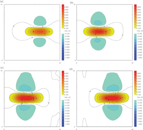
Horizontal wind increments produced by the BFN along the various iterations are displayed at 2000 m in Fig. 6. After the first forward integration, a zonal wind increase of about 0.5 m s⁻¹ is noticed downstream of the observation, and is extending about 5 km eastwards. This spatial extent is consistent with the imposed horizontal scale radius of 1500 m. After the first backward integration, this structure has intensified and is located upstream of the observation location. After four iterations, a dipole structure of the increments is noticeable with two vortices generated North and South of the observation, associated with slower westerly flows corresponding to the model dynamical response to the nudging term. Since only one observation is assimilated at each model level, the increments reflect the horizontal structure of ‘equivalent’ background error covariances as in a variational data assimilation system. Their structure is consistent with the simple 2-D formulation proposed by Daley (1991), assuming an isotropic and completely non-divergent flow. Indeed vertical velocity increments produced during the BFN are small (about 1 cm s⁻¹) and restricted to levels with an observation available (100 and 3000 m). This simple experiment shows the capacity of nudging to develop balanced wind increments (Barwell and Bromley, 1988), using the model dynamics and a homogeneous nudging weight W _xy. The dynamics moves also the increments downstream of the observation. When examining the increments of the zonal wind intensity at the end of the first backward integration (Fig. 7), a similar structure of increments is noticed, with larger magnitude and a position upstream the observation location. Such behaviour is typical of 4-D-Var assimilation that allows increments at the beginning of the time window to be created upstream of the observation when available later in the time window, generating the so-called flow-dependent structure functions (Rabier et al., 1998). The westward propagation of this increment with a slight modification in magnitude is clearly shown when examining its structure and location after the second forward model integration. This explains why the RMSE is minimum in the middle of the assimilation window, since the largest corrections are located near the observation, whereas before that time the maximum is upstream and subsequently downstream.

Fig. 6.  Wind vector increments at 2000 m during the BFN [first forward integration (a), first backward integration (b), fourth backward integration (c) and fifth forward integration (d)]. Maximum vector represented on each graphic legend corresponds to 1.04 m s⁻¹. The ‘X’ corresponds to the observation location.

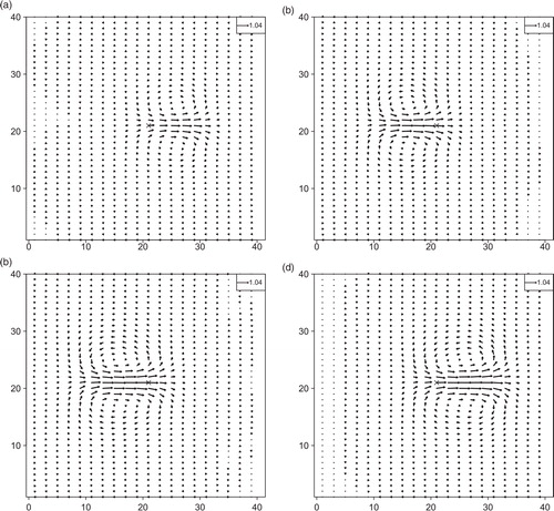
Fig. 7.  Same as Fig. 6 but for the zonal wind increments.

4.1.4. Sensitivity to the vertical length scale R_z.

Given the horizontal size of the domain, the influence of the horizontal radius R _xy has not been studied. Indeed, a significantly larger value than 1500 m would produce increments close to the lateral boundaries of the domain, requiring either a larger domain or a weaker mean flow intensity. In practice, the value of R _xy should depend upon the location of the instrument, with larger values over flat areas than near coastlines or mountainous regions. It could be derived from an ensemble of forecasts as it is done in operational systems for the estimation of the background error covariances.

On the other hand, we have examined the influence of the vertical radius R _z. The value of 100 m set in the previous experiments has been reduced to 10 m in a sensitivity study. When R _z=10 m, each simulated observation influences only one given level. Such an assumption is probably reasonable for UHF wind profiler data which have a vertical resolution around 35 m, higher than that of most numerical models. Since the observed wind profile is uniform above 1000 m the influence of R _z can only be noticed below that level where the wind intensity varies with height. Wind profiler instruments cannot provide useful data below around 100 m. Therefore, it is interesting to examine if an imposed vertical correlation of 100 m could be useful for retrieving near surface wind. The evolution of the wind profile at observation location is shown in Fig. 8, for two BFN experiments with R _z=10 m and R _z=100 m. After one forward integration, with R _z=10 m a better adjustment is noticed above 100 m since each level is only influenced by the observation towards which it should converge, whereas with R _z=100 m each model level also sees the influence of observations below and above, imposing an implicit smoothing. Below 100 m, the lack of downward influence of the first observation above the ground with R _z=10 m leads to a slower wind speed increase with respect to R _z=100 m. In the first backward integration, the nudging term, with R _z=100 m having a contribution down to the surface, allows the profile to get closer to the observation. This is also the case with R _z=10 m above 100 m. Below that level, the vertical wind structure shows unrealistic features only in this model integration. During the next forward integration, the turbulence removes the spurious vertical gradients noticed in the backward integration with R _z=10 m, and the resulting profile after 1 h is similar below 100 m to the one obtained with R _z=100 m.

Fig. 8.  Influence of the vertical length scale R _z on zonal wind profiles at observation location during the first iterations of the BFN. The dashed line indicates the observed profile, the solid line indicates the model profile from a nudging with R _z=10 m, the dash-dotted profile indicates the model profile resulting from a nudging with R _z=100 m. Top left: profiles at initial time, top right: profiles after one forward integration, bottom left: profiles after one backward integration, bottom right: profiles after the second forward integration.

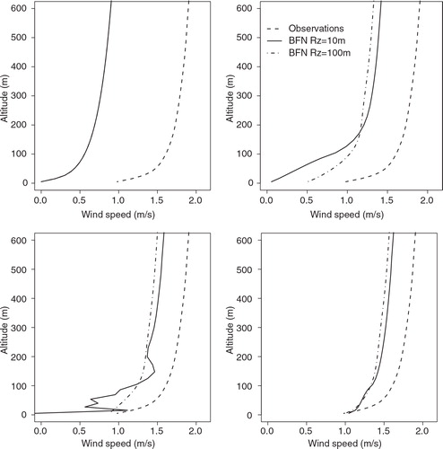
From the above results, it appears that the influence of low-level observations down to the surface helps to produce realistic model fields in areas where the physical processes are important in the forward integration and switched off in the backward integration. On the other hand, the fit to the observations is more difficult with R _z=100 m in regions with significant vertical gradients (below 1000 m). A possible solution to this problem would be to keep a small vertical length scale radius for the wind profiler observations and to include surface wind observations.

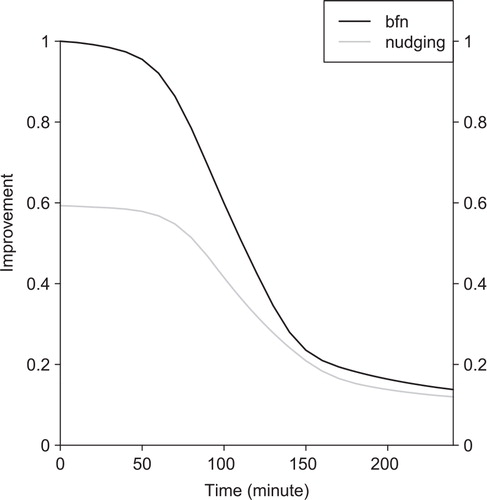
4.1.5. Impact on short-range forecasts.

To assess the ability of the model to maintain the wind increase produced by the assimilation of the observed profile, forecast experiments were performed. The impact of the BFN assimilation system is compared with the nudging effect. For that purpose, three forecast experiments using three different initial conditions were run. The first is the reference experiment starting from initial time and performed without data assimilation. The values obtained at time t of this experiment are noted (u _tref, v _tref). The second forecast experiment starts from the model solution obtained at the end of the assimilation window after the direct nudging (equivalent to 0.5 BFN iteration). The last forecast experiment uses the solution obtained after the forward in time part of the fourth BFN iteration (4.5 iterations) defined hereafter as (u ₀, v ₀). We define a normalised improvement factor as:

where (u _ft, v _ft) is the wind field at time t of the second (nudging) or third (BFN) forecast experiment. Figure 9 shows the evolution of IF over 4 h. As the domain is rather small, the wind changes are mostly carried out of the domain by advection through the eastern boundary. Moreover, the western boundary maintains a constant value of u _ref, forcing the model towards this state. Both simulations maintain the initial value of IF during the first hour of the integration. After that time a significant decrease in the improvement factor is noticed, and it is reduced from 0.95 to 0.35 during the next hour for the BFN. This corresponds to the time when the area of maximum wind increase reaches the eastward boundary of the domain. A much slower decrease takes place afterwards. The direct nudging has a smaller initial IF because it has produced smaller wind increases than the BFN. Therefore, with a slower advection term, the analysis increment is maintained within the experimental domain over a longer period. The decrease is then slower during the second hour of simulation, but the IF remains lower for the direct nudging than for the BFN.

Fig. 9.  Improvement factor (departure in RMS from the initial state) during a 4-h forecast after a direct nudging and a BFN (experiment with constant zonal wind).

4.2. Observations with a wind rotation

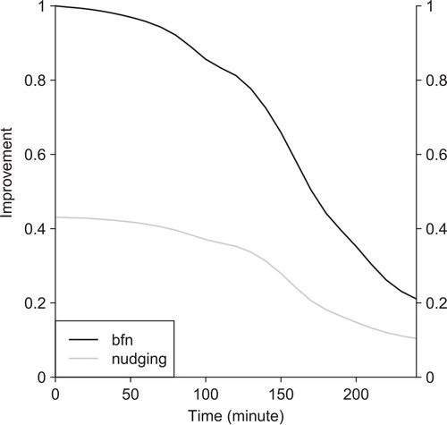
In order to examine the adjustment of the model initial state towards a rapidly changing wind direction, as could occur with low-level wind shear events, the previous westerly wind observation profile of 2 m s⁻¹ has been progressively rotated by 90° counterclockwise within an hour. A set of seven observations sampled every 10 min and starting at initial time are ingested in the nudging scheme with a 5 min temporal window T. Figure 10 shows the evolution of the horizontal wind at the end of forward and backward integrations of the BFN. Starting from a uniform zonal wind (Fig. 10a), the direct nudging leads to a southwesterly wind at the observed location, and up to 5 km downstream with a non-negligible increase in wind intensity (Fig. 10b). A wind increase is also noticed South-West of the observations, which is compensated by a wind decrease in the North-West and south-East regions near the observation. After two BFN iterations (Fig. 10c), the region of westerly wind with increased intensity at the observed location (at time t=0) is surrounded by an area of southwesterly wind in the lower left corner of the domain. This wind structure reveals that, at the initial time, information on the wind rotation present in ‘future’ observations is obtained by the backward integration of the model. The next direct integration (Fig. 10d) intensifies and propagates the patterns noticed at time t=0 westwards. At the observed location, it can be seen that the wind has a more pronounced southerly component than after the first direct nudging. The spatial extent of the wind modification is about 5 km in each direction, which is compatible with the horizontal scale radius (1.5 km) and with the mean advection time (4 km h⁻¹). The existence of stagnation areas close to the observed location (northwestwards and southeastwards) reveals that the nudging constraint does not prevent the model dynamics from generating increments consistent with its equations. The improvement factor IF computed during a 4-h model forecast remains above 0.40 during the first 180 min for the BFN which correspond to the maximum value of the IF maintained for 80 min for the direct nudging (Fig. 11). The zonal wind component has increased less than in the previous experiment (at the expense of meridional wind changes), and there is a southwesterly dominant flow in the central part of the domain (rather than a westerly flow). As a consequence, increments generated during the assimilation experiments are advected north-eastward and then carried out of the domain, through the eastern boundary, more slowly.

Fig. 10.  Wind vector at 2000 m during the BFN iterations with an observation having a 90° rotation in 1 h (from westerly to southerly direction). (a) At initial time, (b) after one forward integration, (c) after two backward integrations and (d) after three forward integrations. Maximum vector represented on each graphic legend corresponds to 1.04 m s⁻¹. The ‘X’ corresponds to the observation location.

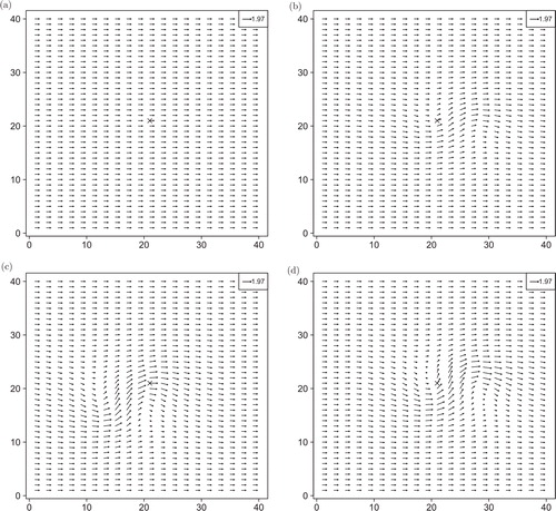
Fig. 11.  Improvement factor (departure in RMS from the initial state) during a 4-h forecast after direct nudging and BFN (experiment with wind rotation).

5. Conclusions and perspectives

The use of high temporally resolved ground-based observations (a few minutes) is still a challenge for current operational Numerical Weather Prediction systems, since it requires efficient data assimilation systems within high-resolution numerical models. The present study makes preliminary steps in this research area. A new data assimilation technique, called BFN, proposed by Auroux and Blum (2005) which fits a model trajectory to available observations over a given time window through iterative direct and backward integrations of a numerical model is tested. The BFN has been examined with the atmospheric numerical mesoscale model Meso-NH (Lafore et al., 1998). This technique has similarities to 4-D-Var, but is much simpler to implement. This method was successfully examined with rather simple models, but not yet with more realistic numerical models including diabatic (irreversible) processes.

First, the BFN is implemented in Meso-NH and tested against simulated observations in order to control its behaviour. The model has been run at small horizontal scale (500 m), and over a short assimilation window (1 h), using low-level wind profile data. It is shown that the BFN is more efficient at correcting the model state than direct nudging since it allows the observations to be seen several times by the model trajectory. The backward integrations allow the observation information to be propagated upstream, whereas the direct nudging can only propagate the information downstream. With a single wind profile observation, it is shown that the convergence of the BFN is reached in five iterations. The contribution of the nudging term to the momentum equations is examined and found to have a smaller magnitude than advection terms, and of comparable magnitude to the vertical diffusion tendencies. Despite running the backward integration with an adiabatic version of the model the convergence is not hampered, even though spurious features have been observed near the surface when no observations are assimilated below a certain level. Finally, an experiment with a rotation of the wind (90° in 1 h) demonstrated the ability of the BFN to find a solution compatible with both the model equations and the observations varying rapidly in time. Forecast integrations subsequent to the analysis period have shown that wind changes can be maintained in the model for around 2 h, corresponding to the advection time through the eastern lateral boundary of the domain.

It is planned to examine the behaviour of the BFN with Meso-NH on real meteorological situations. The surroundings of the Nice airport are of particular interest because of the availability of an operational wind profiler and frequent low-level wind shear hazards. The initial conditions will be taken from an operational atmospheric analysis and surface conditions will be realistic (orography and physiography). First, modelled profiles shifted in time and considered as truth will be assimilated to determine the coefficients to be applied for real conditions and then, observed profiles will be assimilated with the BFN technique. In both cases, particular attention will be paid to the influence of the nudging term compared with model tendencies. Indeed, the nudging relaxation and weighting terms (responsible of the nudging term influence) include the observations and guess errors as well as horizontal correlation. During backward integrations on real cases, the diffusion term will keep the same sign but tests could be done with an inverted sign. With experiments involving real cases, we would like to address the question if high temporal data provided by a wind profiler can modify the initial state of the numerical model to produce better short-range forecasts (<3 h) of wind shear events. This is important over strategic areas like airports, wind farms and for air quality forecasts.

Acknowledgements

This study has been partly funded by a scholarship from the Agence Nationale de la Recherche Technique through a partnership between Météo-France and Degréane-Horizon. We acknowledge Jean-Pierre Claeyman (Degréane-Horizon) for his involvement in initiating the partnership. Technical support and scientific advices from Christine Lac and Valéry Masson were instrumental for the inclusion of the BFN in the Meso-NH model. We would like to express our gratitude to Joël Noilhan (who sadly passed away in October 2010) for his enthusiasm and inspiration during the course of this study. We thank Clara Draper for her careful reading of the manuscript.

References

- Auroux, D. 2008. The back and forth nudging algorithm applied to a shallow water model, comparison and hybridization with the 4D-Var. INRIA Research Report No. 6687. 26 pp.
- Auroux D. Blum J. Back and forth nudging algorithm for data assimilation problems. C. R. Acad. Sci. Ser. I. 2005; 340: 873–878.
- Auroux D. Blum J. A nudging-based data assimilation method: the back and forth nudging (BFN) algorithm. Nonlin. Process. Geophys. 2008; 15: 305–319.
- Barwell B. R. Bromley R. A. The adjustment of numerical weather prediction models to local perturbations. Q. J. R. Meteorol. Soc. 1988; 114: 665–689.
- Benjamin S. Seaman N. A simple scheme for objective analysis in curved flow. Mon. Weather Rev. 1985; 113: 1184–1198.
- Bidet, Y and Schwartz, E. 2006. Modélisation par MésoNH d'une situation de cisaillement de vent sur l'aéroport de Nice. Rapport d’étude DIRSE. Météo-France, 16 pp.
- Bloom S. C. Takacs L. L. Da Silva A. M. Ledvina D. Data assimilation using incremental analysis updates. Mon. Weather Rev. 1996; 124: 1256–1271.
- Boilley, A, Mahfouf, J.-F and Lac, C. 2008. High resolution numerical modeling of low level wind-shear over the Nice-Côte d'Azur airport. Proceedings of the 13th AMS Conference on Mountain Meteorology, 11–15 August 2008, Whistler, BC, Canada.
- Bonavita M. Torrisi L. Marcucci F. Ensemble data assimilation with the CNMCA regional forecasting system. Q. J. R. Meteorol. Soc. 2010; 136: 132–145.
- Bougeault P. Lacarrère P. Parametrization of orographic induced turbulence in a mesobeta scale model. Mon. Weather Rev. 1989; 117: 1872–1890.
- Carpenter K. M. Note on the paper “radiation conditions for the lateral boundaries of limited-area numerical models” by M.J. Miller and A.J. Thorpe. 1982; 108: 717–719.
- Caumont O. Ducrocq V. Wattrelot V. Jaubert G. Pradier-Vabre S. 1D + 3DVar assimilation of radar reflectivity data: a proof of concept. Q. J. R. Meteorol. Soc. 2010; 62: 173–187.
- Courtier P. Thépaut J.-N. Hollingsworth A. A strategy for operational implementation of 4D-Var, using an incremental approach. Tellus. 1994; 120: 1367–1387.
- Cuxart J. Bougeault P. Redelsperger J.-L. A turbulence scheme allowing for mesoscale and large-eddy simulations. Q. J. R. Meteorol. Soc. 2000; 126: 1–30.
- Daley R. Atmospheric Data Analysis. Cambridge University Press, Cambridge.1991
- Deardorff J. W. Numerical investigation of neutral and unstable planetary boundary layers. 1972; 29: 91–115.
- Houtekamer, P. L, Mitchell, H. L, Pellerin, G, Buehner, M, Charron, M and co-authors. 2005. Atmospheric data assimilation with an ensemble Kalman filter: results with real observations. J. Atmos. Sci. 133, 604–620.
- Hug, C, Kaufmann, P and Ruffieux, D. 2010. Verification of COSMO-2 with independent data from a wind profiler. COSMO Newsletter No. 10. 6 pp.
- Kalnay E. Pu Z.-X. Gao J. Application of the quasi-inverse method to data assimilation. 2000; 128: 864–875.
- Lafore, J.-P, Stein, J, Ascencio, N, Bougeault, B, Ducrocq, V and co-authors. 1998. The Meso-NH atmospheric simulation system. Part I: adiabatic formulation and control simulations. Mon. Weather Rev. 16, 90–109.
- Lynch P. Huang X.-Y. Initialization of the HIRLAM model using a digital filter. Ann. Geophys. 1992; 120: 1019–1034.
- Montmerle T. Faccani C. Mesoscale assimilation of radial velocities from Doppler radar in a pre-operational framework. Mon. Weather Rev. 2009; 137: 1937–1953.
- Nielsen-Gammon, J. W, McNider, R. T, Angevine, W. M, White, A. B and Knupp, K. 2007. Mesoscale model performance with assimilation of wind profiler data: sensitivity to assimilation parameters and network configuration. Mon. Weather Rev. 112, D9. 10.3402/tellusa.v64i0.18697.
- Rabier F. Thépaut J.-N. Courtier P. Extended assimilation and forecast experiments with a four-dimensional variational assimilation system. J. Geophys. Res. 1998; 124: 1861–1887.
- Stauffer D. R. Seaman N. L. Use of four-dimensional data assimilation in a limited-area mesoscale model. Part I: experiments with synoptic-scale data. Q. J. R. Meteorol. Soc. 1990; 118: 1250–1277.
- Talagrand, O. 1999. A posteriori evaluation and verification of analysis and assimilation algorithms. Proceedings of the ECMWF Workshop on Diagnosis of Data Assimilation Systems, 2–4 November 1998, Reading, UK, pp. 17–28.
- Torn R. D. Hakim G. J. Performance characteristics of a pseudo-operational ensemble Kalman filter. 2008; 136: 3947–3963.
- Zou X. Navon I. M. Le Dimet F.-X. An optimal nudging data assimilation scheme using parameter estimation. Mon. Weather Rev. 1992; 118: 1163–1186.