Added economic value of limited area multi-EPS weather forecasting applications

ABSTRACT

We compare the GLAMEPS system, a pan-European limited area ensemble prediction system, with ECMWF's EPS over Belgium for an extended period from March 2010 until the end of December 2010. In agreement with a previous study, we find GLAMEPS scores considerably better than ECMWF's EPS. To compute the economic value, we introduce a new relative economic value score for continuous forecasts. The added value of combining the GLAMEPS system with the LAEF system over Belgium is studied. We conclude that adding LAEF to GLAMEPS increases the value, although the increase is small compared to the improvement of GLAMEPS to ECMWF's EPS. As an added benefit we find that the combined GLAMEPS-LAEF multi-EPS system is more robust, that is, it is less vulnerable to the (accidental) removal of one of its components.

• LAM
• EPS
• verification
• probabilistic forecasting
• economic value

1. Introduction

The last decade several mesoscale EPS systems have been developed in Europe running over domains that cover large parts of Europe. Without being exhaustive, we list the following systems in Europe: the GLAMEPS (Iversen et al., 2011), the ALADIN HUNEPS (Horányi et al., 2011), LAEF (Wang et al., 2011a), SREPS (García-Moya et al., 2011), MOGREPS (Bowler et al., 2008), the NORLAMEPS (Aspelien et al., 2011) and the COSMO-LEPS (Montani et al., 2011). These EPS systems are developed in the international collaborations of the European Numerical Weather Prediction (NWP) consortia. For instance, the ALADIN HUNEPS and the LAEF system are developed in the ALADIN consortium and the COSMO-LEPS in the COSMO consortium. The GLAMEPS on the other hand is a collaboration between researchers of the HIRLAM and the ALADIN consortium.

There is a lot of diversification between these systems. First they run on different domains, which overlap each other but never entirely. Secondly, the systems are based on different limited area models, most of them developed within the European NWP consortia. The SREPS, for instance, uses five different models: HIRLAM (HIRLAM Consortium), HRM (DWD), the UM (UKMO), MM5 (PSU/NCAR) and COSMO (COSMO Consortium), whereas HUNEPS is exclusively based on the ALADIN model.

At the RMI we have contributed to both the development of GLAMEPS and LAEF, and thus the data produced by both systems are currently available at the RMI, albeit in a pre-operational mode, and the model domains of both systems cover Belgium. Product development can thus be based on the forecast data of both systems.

For specific applications one does not always need to have the full data of the EPS over the whole domain. An example is wind-energy applications, where only the output of the wind is needed at the height of the wind turbine. Delivering such data from all the members of different ensemble systems, for such singular locations, does not require a huge data set to be transferred, at least not compared to the full sets representing the model states of the members.

Given that there already exist so many EPS systems within the ALADIN and HIRLAM consortia, it seems more advantageous for the RMI to use the available model output of the existing models rather than to develop another Belgian mesoscale EPS system, and, it seems, at the same time, a more efficient use of resources to contribute to the GLAMEPS and LAEF. Research is needed to study which data to use and how to optimally use the data, in combination with robustness studies. The present paper presents a first study of this. Here, we study only the data from the GLAMEPS, LAEF and ECMWF EPS ensembles, correct them using a simple bias correction, and combine the ensembles by adding all the members together with equal weight. More advanced forms of combining and calibrating the ensembles and study of data from other ensembles will be left to future publications.

The aim of the present paper was (1) to verify the quality of the GLAMEPS system, (2) study the added economic value when adding the LAEF model output to the GLAMEPS and (3) study the robustness of the combined system. By robustness we mean the following: suppose one of both systems will operationally drop out, then what will be the loss in quality/value for that particular run? In order to calculate the economic value, we also introduce a new relative economic value score suitable for ‘continuous’ forecasts (as opposed to forecasts for binary events). This score is especially useful for users of weather forecasts that are not interested in forecasting events, but rather are interested in forecasting amounts, e.g. wind energy producers, electricity suppliers, etc.

The paper is organised as follows. In Section 2 we describe the forecast and observation data used in this paper. We then explain the method used to compute the (relative) economic value in Section 3. The quality of the GLAMEPS system is compared with ECMWF's EPS in Section 4. Next, we study the added value of the LAEF system to GLAMEPS in Section 5, and investigate the robustness of the combined system in Section 6. Finally, Section 7 contains a summary of the paper with conclusions and directions for future research.

2. Data and model descriptions

In this paper, we use forecast data from three different ensemble prediction systems, namely ECMWF's EPS, GLAMEPS and LAEF, over the period 1 March 2010 until 29 December 2010. We describe each system in turn.

The EPS system from ECMWF (which we denote here by ECEPS to avoid confusion with the generic use of the term EPS) is a global system with a control and 50 perturbed members. Since 26 January 2010 it has a horizontal resolution of 32 km. The system underwent a significant upgrade on 24 June 2010 with the introduction of Ensemble Data Assimilation (EDA) for the perturbations (Buizza et al., 2008, 2010). A further upgrade of the EPS occurred on 9 November 2010, see the ECMWF website for detailed information.

The ALADIN-LAEF system (Wang et al., 2011a, 2011b), here denoted LAEF for short, is an operational limited area EPS based on the ALADIN NWP model, and uses ECEPS for initial conditions and lateral boundaries. It has a horizontal resolution of 18 km, and has 17 members. One member called the control is a downscaling (with a version of the ALADIN model) of the ECEPS control forecast, while the other 16 are the so-called perturbed members. Their atmospheric perturbations are the result of a breeding-blending technique. Small-scale perturbations are generated using a breeding method with the ALADIN model, and are then combined with the large-scale perturbations of the first 16 ECEPS perturbed members. Surface perturbations are also introduced for the 16 perturbed members, using a Non-Cycling Surface Breeding Method (Smet, 2009; Wang et al., 2010, 2011b). Finally, model uncertainty is taken into account by using different ALADIN physics configurations for each member; see Wang et al. (2011a) for a detailed description of the ALADIN model versions used.

GLAMEPS is a multimodel LAM-EPS. It combines members from the ALADIN model and two versions of the HIRLAM model with members interpolated from ECEPS. A test version of this system was described in the study of Iversen et al. (2011). Since March 2010, a pre-operational version has been running twice daily. Compared to the test version described in the study of Iversen et al. (2011), there are a few notable differences:

• The initial and boundary conditions are taken directly from ECEPS, not from the targeted global EPS system EuroTEPS.

• The ALADIN and HIRLAM components of the system each run 12 perturbed members and a control. Combined with the ECEPS members themselves (which are interpolated to the common grid), this gives a total of 52 members (including the control members in the ensemble).

• No calibration is applied to the member forecasts.

We denote the ALADIN component of GLAMEPS as AladEPS here. It is a simple downscaling (without data-assimilation) of the control and the first 12 perturbed members of ECEPS, using a single version of the ALADIN model, and therefore considerably less sophisticated than the LAEF system. It has on the other hand a higher resolution of 12.9 km. The two HIRLAM components are denoted as HirEPS_K and HirEPS_S (as in the study of Iversen et al. 2011); they use the HIRLAM model with two different cloud physics parameterisations. The control run of each model version is produced using the ECEPS control and a 3DVar assimilation cycle, while the runs of the 12 perturbed members are simply a downscaling (without data-assimilation) of the first 12 ECEPS perturbed members with the two versions of the HIRLAM model. They have a horizontal resolution of 12.8 km. Finally, the ECEPS component of GLAMEPS simply consists of the control and the first 12 members of ECEPS, and is denoted as ECEPS13 as a reminder that only 13 (of the 51) members of ECEPS are a part of GLAMEPS.

The forecast data were compared against observations coming from 10 standard stations in Belgium (see Fig. 1). To create forecast data at the station locations we used a bilinear interpolation for all the models. We only look at 2 m temperature T _2m and 10 m wind S _10m in this paper. Because precipitation is of a more local nature, using a combination of radar and rain gauge data as observations is more appropriate. This will be left for a future publication.

Fig. 1.  Map of Belgium with latitude/longitude axes. Belgian weather stations used in this study are denoted with a dot, together with their place name and their WMO number in parentheses.

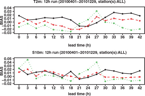
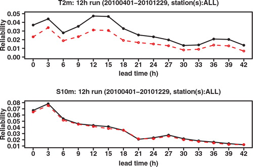
Because of differences in model height and station height, other environmental specifics of the station locations not resolved in the model, and model imperfections, there will be systematic biases present in the forecast data when compared with the station observation data. A simple 28 d sliding bias correction was applied to the forecast data. For each forecast date, run time, lead time and station, we calculated the bias over the previous 28 d and subtracted it, setting negative wind speeds to zero. This removes most of the bias; in Fig. 2 you can see the remaining bias of the bias corrected T _2m and S _10m for the 12 h run. Results for the 0 h run are similar (not shown).

Fig. 2.  BIAS of ensemble mean ECEPS (black full line), ensemble mean GLAMEPS (red dashed line) and ensemble mean LAEF (green dotted line) for bias corrected T _2m and S _10m (run=12 h).

All scores in this paper are calculated using these bias corrected data, averaged over the 10 stations and over the forecast period 1 April 2010 until 29 December 2010 (with observations used from 1 April 2010 until 31 December 2010). Even though significant changes occurred to the ECEPS during this period, which might also impact GLAMEPS and LAEF since they use ECEPS lateral boundaries and initial conditions, these changes do not have much impact on the results of this study. We have calculated scores over the periods 1 April 2010 until 20 June 2010, 1 July 2010 until 31 October 2010 and 15 November until 29 December 2010, and did not find any qualitative differences that would lead us to change our conclusions. We therefore only show plots of scores averaged over the whole verification period. Moreover, because the results of the 0 h and 12 h run are very similar, we show only results of the 12 h run. For a few cases were the 0 h run gives some added information, we have supplied supplemental figures as supporting information, which can be viewed on the publisher's website. Finally, we have also calculated the scores using the raw data, i.e. without doing the bias correction. We saw no qualitative differences with the results of the bias-corrected data, showing that none of the main results in the paper are a result of the bias correction itself. We therefore only show results using the bias corrected data in this paper. Quantitatively, the bias correction brings the scores of GLAMEPS and ECEPS somewhat closer together, because ECEPS has a somewhat larger bias. Due to ECEPS lower resolution, this is to be expected when you compare station observations with interpolated model data. The bias correction makes the comparison of models of different resolution fairer.

3. Method used to compute the economic value (CREV)

Relative economic value is often calculated for binary events, e.g. T _2m<0 °C, S _10m>5 m s⁻¹, etc., using the static cost-loss model (Richardson, 2000, 2003; Zhu et al., 2002). Instead, we calculate relative economic value for the continuous variables directly, i.e. without choosing thresholds, by using a continuous version of the static cost-loss model. We refer the reader to the Appendix for a detailed explanation. Instead of thresholds, a loss function has to be specified. The relative (potential) economic value scores in this paper are calculated using a loss function that is linear in the absolute difference between forecast and observed (actual) value:1

where Loss is the loss function, x ^a and x ^f are the actual (observed) values and predicted (forecast) values, respectively, and cl parametrises the relative importance of over- and under-forecasting errors. Here x ^f can be a deterministic forecast, or the ensemble mean of an EPS system, but it can also be an optimal value based on a probabilistic weather forecast. Given a probability forecast, one can derive a value x ^f that will minimise the loss function. For the linear loss function in eq. (1), the optimal x ^f are quantiles, i.e. one should choose x ^f such that:2

assuming the probability forecasts are perfectly reliable. Essentially this loss function was also used in the works of Smith et al. (2001); Roulston et al. (2003); Pinson et al. (2007) to study the economic value of weather forecasts in the energy market.

Relative economic value of a forecast system is defined in the usual way:3

where is the loss averaged over time or over several locations, which a risk neutral decision maker will want to minimise. Here is the average loss of the forecast system under study, while and are the average loss of a reference forecast system and a perfect forecast system, respectively. For the loss function in eq. (1), we have .

As reference (probability) forecasts we take a normal and Weibull distribution for T _2m and S _10m respectively, with mean and standard deviation of the distribution equal to the monthly mean and monthly standard deviation of the sample observations, respectively. We refer to this as the sample climatology and denote the relative economic value calculated as in eq. (3) with V _clim . The probability forecasts of the models are constructed by estimating quantiles from the model member forecasts, using the quantile function in R, with the default ‘type 7’ method (Frohne and Hyndman, 2009; R Development Core Team, 2009). For an ensemble of N (ordered) forecasts x _i , with i=1, …, N and x ₁ ≤ …≤ x _i ≤ …≤ x _N , the estimate for the k-th q-quantile Q _k/q is calculated as:4

with and the smallest integer not greater than h. When h is an integer, the quantile estimate is just the hth smallest forecast value. Otherwise it is a linearly interpolated value.

We call the above score the ‘CREV’ score, as a shorthand for Continuous Relative Economic Value score, since it is a natural generalisation of the relative economic score for binary forecasts to the continuous case. In the next sections we calculate the (potential) CREV score for T _2m, and S _10m by taking x ^a to be the T _2m, and S _10m as observed in the 10 weather stations, and x ^f , the optimal forecast value for the location of the weather stations, based on the probability forecasts derived from the EPS.

4. Verification of GLAMEPS (over Belgium)

In this section we discuss some comparisons of ECEPS vs. GLAMEPS. The difference with the previous results given in the study of Iversen et al. (2011) lies in the much longer verification period (10 months) and the focus on one smaller verification domain (Belgium) instead of the whole GLAMEPS domain. As mentioned before, we show only the results of the 12 h run in this section, as the scores of the 0 h run are very similar. The results that we obtain are in line with previous results obtained in the study of Iversen et al. (2011). In general they show a clear improvement of scores with GLAMEPS w.r.t. ECEPS.

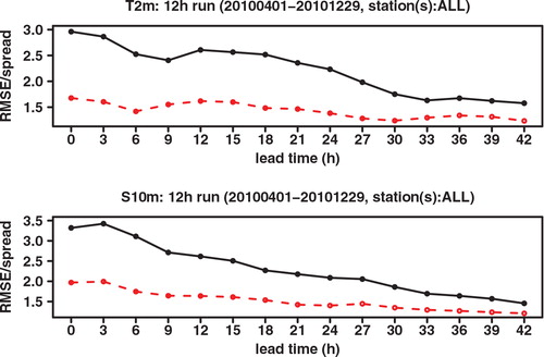
In Fig. 3 we compare the root mean square error (RMSE) of the ensemble mean forecasts of GLAMEPS and ECEPS for T _2m (top graph) and S _10m (bottom graph), for forecast lead times up to 42 h (the maximum range of GLAMEPS during the test period). Quite clearly, the RMSE of the ensemble mean of GLAMEPS is lower than that of ECEPS, both for T _2m and S _10m. It may be seen, however, that the difference starts to diminish as the forecast range increases.

Fig. 3.  RMSE of ensemble mean ECEPS (black full line) and ensemble mean GLAMEPS (red dashed line), for bias corrected T _2m and S _10m (run=12 h).

This convergence at longer forecast ranges is even more visible in Fig. 4. There we compare the ratio of the RMSE (as plotted in Fig. 3) with the spread (square root of the ensemble variance around the mean). Ideally, this ratio should be 1. A higher value means that the ensemble is underdispersive. While both ECEPS and GLAMEPS are underdispersive, the ratio for GLAMEPS is much closer to one. At longer forecast ranges, the ratio of ECEPS comes closer to that of GLAMEPS. This should not surprise us. ECEPS is not aimed as much at short-term forecasts. The singular vectors used in the perturbations of ECEPS are optimised for a lead time of 48 h.

Fig. 4.  Ratio of RMSE to spread ratio of ECEPS (black full line) and GLAMEPS (red dashed line) for bias corrected T _2m and S _10m (run=12 h).

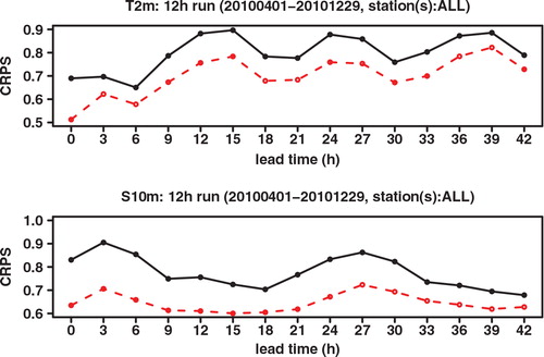
We next look at the Continuous Ranked Probability Score (CRPS), which may be interpreted as an integration of the Brier score over all possible threshold values. See, for example, Hersbach (2000) for a definition and for the decomposition of the CRPS into different components. As shown in Fig. 5, the CRPS of GLAMEPS is significantly lower than that of ECEPS. Especially for S _10m we can see that the difference decreases for longer forecast ranges. There also seems to be a daily cycle in the score, which can also be seen in the RMSE.

Fig. 5.  CRPS of ECEPS (black full line) and GLAMEPS (red dashed line) for bias corrected T _2m and S _10m (run=12 h).

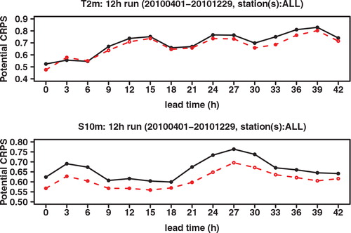
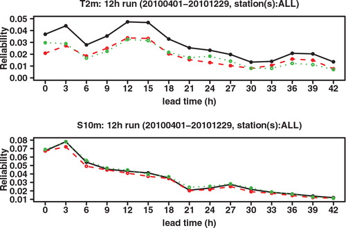
As shown in the study of Hersbach (2000), the CRPS may be decomposed into a reliability part and a resolution/uncertainty part, also called the potential CRPS. This decomposition is similar to the decomposition of the Brier score. Figure 6 compares the reliability component of the CRPS, while Fig. 7 compares the potential CRPS (that is, the CRPS with the reliability component extracted). These graphs show that the better CRPS of GLAMEPS, especially at shorter forecast ranges, is mainly (but not exclusively) due to improved reliability. We also see that the reliability of ECEPS comes closer to that of GLAMEPS at longer forecast ranges.

Fig. 6.  Reliability component of CRPS of ECEPS (black full line) and GLAMEPS (red dashed line) for bias corrected T _2m and S _10m (run=12 h).

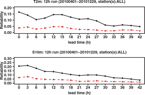
Fig. 7.  Potential CRPS of ECEPS (black full line) and GLAMEPS (red dashed line) for bias corrected T _2m and S _10m (run=12 h).

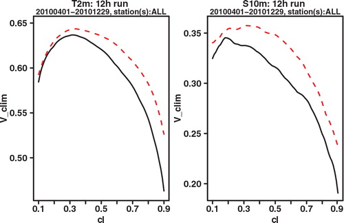
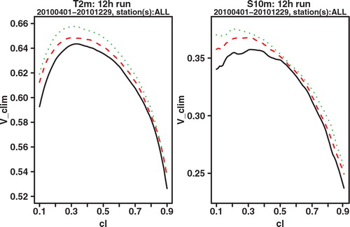
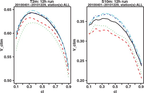
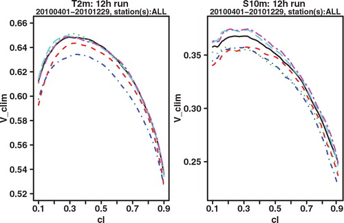
As a final verification score, we compare the potential CREV scores. Potential in this context again means that it is the score one could get if the system was made perfectly reliable. For each cl, the potential CREV is calculated by taking x ^f not the cl-quantile as in eq. (2), which would be optimal if the system was perfectly reliable, but the quantile that gives the highest CREV score. This is completely analogous to how the potential (relative) economic value score is calculated in the standard binary cost-loss scenario. Figures 8 and 9 show the plot of potential CREV for lead times of 24 and 42 h, respectively. Both the figures show a clear improvement for GLAMEPS, but one may also see that the difference with ECEPS is smaller at the longest forecast range (42 h).

Fig. 8.  Potential CREV relative to (sample) climatology of ECEPS (black full line) and GLAMEPS (red dashed line) for bias corrected T _2m and S _10m (run=12 h, lead time=24 h).

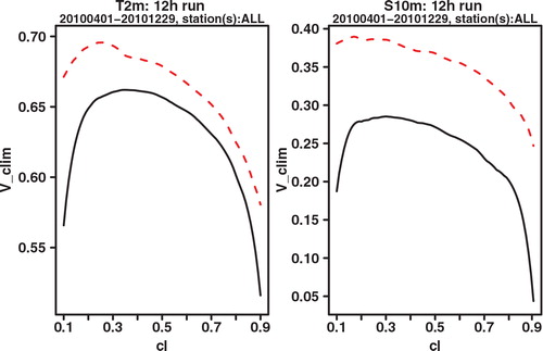
Fig. 9.  Potential CREV relative to (sample) climatology of ECEPS (black full line) and GLAMEPS (red dashed line) for bias corrected T _2m and S _10m (run=12 h, lead time=42 h).

Using a block bootstrap technique we have also constructed 95% confidence intervals for the differences in RMSE and CRPS. They show that there is a statistically significant difference at the 5% level between the scores of GLAMEPS and ECEPS; see Figs. 10 and 11.

Fig. 10.  Confidence interval (95%) for the difference in RMSE of GLAMEPS vs. ECEPS (black full line with circle) and GLAMEPS-LAEF vs. GLAMEPS (red dashed line with triangle) for bias corrected T _2m and S _10m (run=12 h).

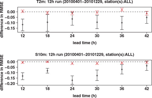
Fig. 11.  Confidence interval (95%) for the difference in CRPS of GLAMEPS vs. ECEPS (black full line with circle) and GLAMEPS-LAEF vs. GLAMEPS (red dashed line with triangle) for bias corrected T _2m and S _10m (run=12 h).

5. Added value of LAEF and ECEPS to GLAMEPS

In this section, we investigate whether adding LAEF and/or ECEPS to GLAMEPS increases its value. We combine the models in the simplest way possible, by just pooling all members together and treating them as equally likely members of a single ensemble. GLAMEPS already contains the control and first 12 members of ECEPS. When we add ECEPS to the GLAMEPS-LAEF ensemble, we only add the ECEPS members that are not already included in the GLAMEPS ensemble. The GLAMEPS-LAEF ensemble therefore contains 69 (=52+17) members, while the ECEPS-GLAMEPS-LAEF ensemble consists of 107 (=51−13+69) members.

5.1. Added value LAEF to GLAMEPS

We find that overall LAEF adds value to GLAMEPS, both for T _2m and S _10m. This can be seen for instance in the CRPS score shown in Fig. 12 and its reliability component in Fig. 13. Also potential CREV shows a small improvement at most lead times (see e.g. Figs. 14 and 15). However, the improvement is clearly small compared to the improvement of GLAMEPS to ECEPS. Overall the improvement seems to be a bit bigger for S _10m than for T _2m. It was already noted in Iversen et al. (2011) that S _10m ALADIN forecasts are very good compared to other components of GLAMEPS. Adding LAEF increases the weight of ALADIN models in GLAMEPS. One can also see that for T _2m, the difference in CRPS mainly comes from an improved reliability, which comes at the cost of a slightly reduced resolution at about half of the lead times. For S _10m, on the other hand, the difference in CRPS is mainly due to an improved resolution. Even though the difference between GLAMEPS and GLAMEPS-LAEF is small, we think it cannot be discounted completely, as it is seen quite consistently over all lead times. Moreover, the confidence intervals show that the difference in CRPS between GLAMEPS-LAEF and LAEF is statistically significant at the 5% level, at most lead times, although not for all, both for T _2m and S _10m; see Fig. 11. However, for the differences in RMSE, which only compares the ensemble means and not the whole probability distribution like CRPS, the results are not statistically significant at the 5% level; see Fig. 10.

Fig. 12.  CRPS of GLAMEPS (black full line), GLAMEPS-LAEF (red dashed line) and ECEPS-GLAMEPS-LAEF (green dotted line) for bias corrected T _2m and S _10m (run=12 h).

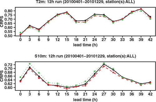
Fig. 13.  Reliability component of CRPS of GLAMEPS (black full line), GLAMEPS-LAEF (red dashed line) and ECEPS-GLAMEPS-LAEF (green dotted line) for bias corrected T _2m and S _10m (run=12 h).

Fig. 14.  Potential CREV relative to (sample) climatology of GLAMEPS (black full line), GLAMEPS-LAEF (red dashed line) and ECEPS-GLAMEPS-LAEF (green dotted line) for bias corrected T _2m and S _10m (run=12 h, lead time=24 h).

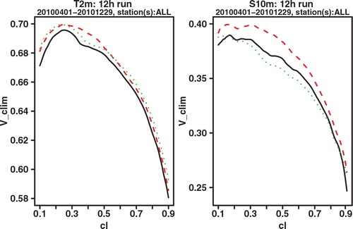
Fig. 15.  Potential CREV relative to (sample) climatology of GLAMEPS (black full line), GLAMEPS-LAEF (red dashed line) and ECEPS-GLAMEPS-LAEF (green dotted line) for bias corrected T _2m and S _10m (run=12 h, lead time=42 h).

In Figs. 16 and 17, we compare LAEF with the AladEPS component of GLAMEPS. Because LAEF contains 17 members, while AladEPS only contains 13 members, we also plotted scores for LAEF13, which is a reduced version of LAEF, consisting only of the control and the first 12 perturbed members of LAEF. The figures clearly show that LAEF scores considerably better than AladEPS, which a priori could be expected since LAEF is much more sophisticated. Because the scores of LAEF13 are only slightly worse than those of LAEF, we can conclude that the better performance of LAEF compared to AladEPS is indeed mainly due to LAEF being a more advanced system, not due to the four extra members.

Fig. 16.  CRPS of LAEF (black full line), LAEF13 (red dashed line) and AladEPS (green dotted line) for bias corrected T _2m and S _10m (run=12 h).

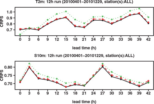
Fig. 17.  Reliability component of CRPS of LAEF (black full line), LAEF13 (red dashed line) and AladEPS (green dotted line) for bias corrected T _2m and S _10m (run=12 h).

However, when we add the other components of GLAMEPS, i.e. we compare GLAMEPS to GLAMEPS-LAEF without the AladEPS component, and we now see that both systems are much more similar in quality; see Figs. 18 and 19. Because of the other models in GLAMEPS, perhaps the weaknesses of AladEPS become less important. It also suggests that the added value of LAEF to GLAMEPS is in large part due to giving extra weight to the ALADIN component in GLAMEPS, and that a similar effect could be obtained by either increasing the number of AladEPS members in GLAMEPS, or a form of calibration that gives extra weight to the AladEPS members in GLAMEPS. For instance a calibration using Bayesian model averaging, BMA (Raftery et al., 2005), might do this naturally. Another possibility is that the positive effects of LAEF are masked by the other models, and that increasing the weight of LAEF in GLAMEPS-LAEF might make its benefits more pronounced. A more detailed investigation of these issues is beyond the scope of this paper and will be kept for a future publication. Finally, note that CRPS and its reliability component are much improved when we compare the scores of GLAMEPS shown in Figs. 18 and 19 with the scores of AladEPS shown in Figs. 16 and 17, showing that the other models in GLAMEPS are good additions to the AladEPS.

Fig. 18.  CRPS of GLAMEPS (black full line) and GLAMEPS-LAEF without AladEPS (red dashed line) for bias corrected T _2m and S _10m (run=12 h).

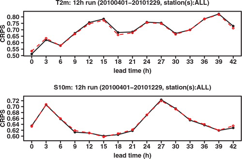
Fig. 19.  Reliability component of CRPS of GLAMEPS (black full line) and GLAMEPS-LAEF without AladEPS (red dashed line) for bias corrected T _2m and S _10m (run=12 h).

5.2. Added value ECEPS to GLAMEPS-LAEF

We now investigate whether adding the remaining 38 ECEPS members not already contained in GLAMEPS can add further value. For T _2m, we find that ECEPS indeed adds a little value, as can be seen for instance in the CRPS score shown in Fig. 12, and potential CREV shown in Figs. 14 and 15. Reliability is also improved compared to GLAMEPS at all lead times, but slightly worse than GLAMEPS-LAEF at some lead times (see Fig. 13). On the other hand, for S _10m, we find that adding the remaining ECEPS members tends to deteriorate the system, especially in the first 24 h, see the CRPS score shown in Fig. 12, and the potential CREV shown in Fig. 15. We think this is mainly because adding more ECEPS members indirectly decreases the weight of the ALADIN members in the system, which were shown to be of higher quality than the other GLAMEPS components for S _10m forecasts in the study of Iversen et al. (2011). At longer lead times, we see that the effect of adding the remaining ECEPS members becomes more positive. For the 12 h run, the S _10m forecast of ECEPS-GLAMEPS-LAEF at 42 h lead time even performs best; see e.g. Figs. 12 and 15. On the other hand, for the 0  h run, adding the remaining ECEPS members still has a small negative effect at 42 h lead time, see Figs. S1 and S2 in the supporting information. However, the effect is clearly a lot less negative than at early lead times. This better performance of ECEPS with lead time was already noticed in the previous section, where we compared GLAMEPS with ECEPS.

Finally, from adding ECEPS to GLAMEPS-LAEF, we learn that adding different ensembles together does not necessarily increase the value of the system. The added value of LAEF to GLAMEPS is thus not a trivial thing, i.e. not just due to increasing the number of members in the ensemble.

6. Robustness

In this section we study the impact of removing one of the components of the (multi-)EPS system, i.e. the robustness of the system. We will study GLAMEPS and GLAMEPS-LAEF.

6.1. Robustness of GLAMEPS

As we described in detail in Section 2, GLAMEPS has four main components, an ALADIN component, denoted as AladEPS, two HIRLAM components HirEPS_K and HirEPS_S and an ECEPS component denoted as ECEPS13, as a reminder that only the control and first 12 members of ECEPS are a part of GLAMEPS. In operational applications, one of these components may be subject to a failure and fall out (as one block).

For the T _2m forecasts, we find that removing ECEPS13 has the biggest negative impact in all scores, with removal of AladEPS being a close second, see Figs. 20–22 for the CRPS and CREV scores of the 12 h run, and Figs. S3–S5 in the supporting information for the corresponding scores of the 0 h run. Note that while in the CREV score of the 12 h run at 24 h lead time, a removal of AladEPS has the biggest impact, this is not the case in the 0 h run, where a removal of ECEPS13 has the biggest negative impact. Also note that if a block falls out due to some operational failure, it will fall out for all lead times. When looking at the CRPS scores over all lead times (see top panel of Fig. 20 and Fig. S3 again), we think it is fair to say that a removal of ECEPS13 has the biggest overall impact on T _2m.

Fig. 20.  CRPS of GLAMEPS (black full line), GLAMEPS without AladEPS (red dashed line), GLAMEPS without ECEPS13 (green dotted line), GLAMEPS without HirEPS_K (blue dash dotted line) and GLAMEPS without HirEPS_S (light blue big dashed line) for bias corrected T _2m and S _10m (run=12 h).

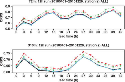
Fig. 21.  Potential CREV relative to (sample) climatology of GLAMEPS (black full line), GLAMEPS without AladEPS (red dashed line), GLAMEPS without ECEPS13 (green dotted line), GLAMEPS without HirEPS_K (blue dash dotted line), and GLAMEPS without HirEPS_S (light blue big dashed line) for bias corrected T _2m and S _10m (run=12 h, lead time=24 h).

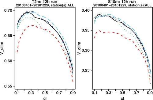
Fig. 22.  Potential CREV relative to (sample) climatology of GLAMEPS (black full line), GLAMEPS without AladEPS (red dashed line), GLAMEPS without ECEPS13 (green dotted line), GLAMEPS without HirEPS_K (blue dash dotted line) and GLAMEPS without HirEPS_S (light blue big dashed line) for bias corrected T _2m and S _10m (run=12 h, lead time=42 h).

For the S _10m forecasts, it should be no surprise given the previous sections that a removal of AladEPS has the biggest negative impact. See Figs. 20–22 for the CRPS and CREV scores of the 12 h run, and supplemental Figs. S3–S5 for the corresponding scores of the 0 h run.

Looking at these figures, one might also notice that a removal of one of the HIRLAM components sometimes seems to have a beneficial effect. However, this is not consistently true for all lead times, and the effect is small compared to a removal of the most important component of the system. It might be accidental or simply an indirect effect, by removing one of the HIRLAM components, the most important component of the system automatically gets more weight. Probably not too much attention should be paid to it. We think it is much more meaningful to look for the component that has the biggest negative impact when removed. In that case we get a clear consistent picture.

6.2 Robustness of GLAMEPS-LAEF

Let us now redo the exercise of the previous section on the GLAMEPS-LAEF ensemble. When looking at the CRPS plot for T _2m shown in the top panel of Fig. 23, we see clearly that over all lead times a removal of ECEPS13 has the biggest negative impact, as was also the case for the GLAMEPS ensemble. This can also be seen in the potential CREV plots, left panels of Figs. 24 and 25. Comparing the CRPS plot in the top panel of Fig. 23 with the CRPS plot in the top panel of Fig. 20 we also see that the negative impact of a removal of AladEPS is reduced. There is now only one model that has a big impact over all lead times.

Fig. 23.  CRPS of GLAMEPS-LAEF (black full line), GLAMEPS (red dashed line), GLAMEPS-LAEF without AladEPS (green dotted line), GLAMEPS-LAEF without ECEPS13 (blue dash dotted line) and GLAMEPS-LAEF without HirEPS_K (light blue big dashed line) and GLAMEPS-LAEF without HirEPS_S (pink big dash dotted line) for bias corrected T _2m and S _10m (run=12 h).

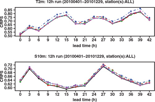
Fig. 24.  Potential CREV relative to (sample) climatology of GLAMEPS-LAEF (black full line), GLAMEPS (red dashed line), GLAMEPS-LAEF without AladEPS (green dotted line), GLAMEPS-LAEF without ECEPS13 (blue dash dotted line) and GLAMEPS-LAEF without HirEPS_K (light blue big dashed line) and GLAMEPS-LAEF without HirEPS_S (pink big dash dotted line) for bias corrected T _2m and S _10m (run=12 h, lead time=24 h).

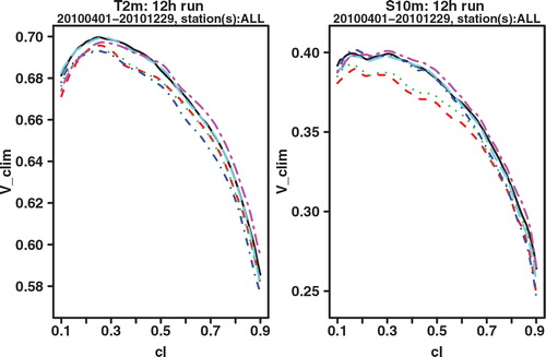
Fig. 25.  Potential CREV relative to (sample) climatology of GLAMEPS-LAEF (black full line), GLAMEPS (red dashed line), GLAMEPS-LAEF without AladEPS (green dotted line), GLAMEPS-LAEF without ECEPS13 (blue dash dotted line) and GLAMEPS-LAEF without HirEPS_K (light blue big dashed line) and GLAMEPS-LAEF without HirEPS_S (pink big dash dotted line) for bias corrected T _2m and S _10m (run=12 h, lead time=42 h).

When we look at the S _10m forecasts we see something even more interesting. For CRPS now there is no single model that has clearly the biggest negative impact on removal (indicating the system is more robust), see Fig. 23. Removing a single component gives negative impacts at some lead times and positive at other lead times.

We conclude that adding LAEF makes GLAMEPS more robust, especially for S _10m. The negative impact of a removal of AladEPS becomes considerably smaller, because LAEF acts as a backup. There are now 2 ALADIN components and 2 HIRLAM components.

7. Summary and conclusions

We compared GLAMEPS 2 m temperature (T _2m) and 10 m wind speed (S _10m) forecasts for Belgium with ECEPS (the EPS of ECMWF) over a 10-month period (9 months for the bias corrected data), using various verification scores, and found GLAMEPS performed considerably better than ECEPS. Reliability, CRPS, RMSE of ensemble mean and the RMSE to spread ratio were all much better for GLAMEPS, in agreement with the results of Iversen et al. (2011). As could be expected, since GLAMEPS is designed for the short-term and ECEPS more for the mid-term, the difference between GLAMEPS and ECEPS decreased with lead time. This was especially the case for the reliability and RMSE to spread ratio. Our study differs from those of Iversen et al. (2011) by the much longer verification period (10 months vs. 7 weeks) and the smaller domain (Belgium vs. the full GLAMEPS domain).

We also introduced a new relative economic value score for continuous variables (CREV), which is a natural generalisation of the commonly used relative economic value for binary forecasts (Richardson, 2000, 2003; Zhu et al., 2002). It has the advantage that no thresholds have to be chosen (to reduce the forecast to a binary event), and could be used for various applications where users are not interested in binary events, but rather in forecasting amounts. For instance in the energy market, it can be used to estimate the relative economic value of weather forecasts for wind power forecasting (Roulston et al., 2003; Pinson et al., 2007) and (temperature dependent) energy demand (Smith et al., 2001). The results of potential CREV agreed with the more traditional verification scores and showed GLAMEPS has considerably more potential relative economic value than ECEPS.

We then studied whether adding the LAEF and ECEPS system to GLAMEPS could further improve the forecasts. Both for T _2m and S _10m we found that LAEF did add value to GLAMEPS. Even though the improvement was small compared to the improvement of GLAMEPS over ECEPS, we found the difference in CRPS score to be statistically significant at the 5%level for most lead times, although not all. Further adding ECEPS to the GLAMEPS-LAEF ensemble gave mixed results. For T _2m there was overall still a little improvement, although it was less clear than the improvement of GLAMEPS-LAEF over GLAMEPS, but for S _10m the scores deteriorated, especially in the first 24 h. We suspect this is mainly because adding more ECEPS members automatically decreases the weight of the ALADIN models in the ensemble, which were shown to be of higher quality than the other GLAMEPS components for the S _10m forecasts in Iversen et al. (2011).

Finally, we investigated the robustness of the GLAMEPS and GLAMEPS-LAEF ensemble, i.e. the impact of a removal of one of its components (e.g. due to some operational failure) on the value of the ensemble. This led to the conclusion that adding LAEF to GLAMEPS would, in addition to the (possibly) increased value, also lead to a more robust system. Although the added value of LAEF was not significant at all lead times, the fact that it also leads to a more robust system, and that LAEF is more sophisticated than AladEPS in GLAMEPS, suggest that using LAEF together with GLAMEPS where both are available should be considered. Moreover, even though the added value of LAEF to GLAMEPS turned out to be small for the T _2m and S _10m forecasts over Belgium, given that LAEF is more sophisticated than AladEPS, it might lead to more value for other meteorological variables, e.g. precipitation, for extreme event forecasting, and/or over other geographical areas than Belgium. On the other hand, we also found that while LAEF scores considerably better than AladEPS, the difference between the two models becomes a lot smaller when the other components of GLAMEPS are added. When the other models in GLAMEPS are added, the weaknesses of AladEPS compared to LAEF become less important. We suspect that the added value of LAEF to GLAMEPS is in large part due to giving more weight to the ALADIN models in GLAMEPS, especially in the S _10m case. Producing more AladEPS members or increasing the weight of AladEPS, perhaps using BMA (Raftery et al., 2005), might therefore be another way to increase the value of GLAMEPS. On the other hand, it might also be possible that some of the positive effects of LAEF are masked by the other GLAMEPS models. In this case, increasing the weight of LAEF in a GLAMEPS-LAEF ensemble might be beneficial. These are interesting directions for future research.

The present study should also be extended for all available EPS data over Belgium. For instance it is useful to set up a product based on EPS, GLAMEPS, LAEF, HUNEPS, and SREPS, since most of these model are somehow developed in the context of the two ALADIN and HIRLAM consortia. In addition more research is needed to determine the best way of combining and calibrating different LAM-EPS systems. Finally, we plan to look into the verification of precipitation using a combination of radar and rain-gauge data over Belgium.

Acknowledgements

The authors would like to thank Florian Weidle for help with the LAEF data on the Mars archive, and the many people that worked on developing GLAMEPS, LAEF and ECMWF's EPS, without whom this work would not have been possible. We also would like to thank two anonymous reviewers for their many helpful comments on the manuscript. This work was supported by the Belgian Science Policy (BELSPO), project 2SPPFOCUS: MO/34/019.

Notes

¹This is not as restrictive as it may look. For instance, while energy demand depends on several weather variables (temperature, cloud cover, wind speed,…), the object of forecast interest is still only one variable, namely the energy demand.

Appendix A: Relative economic value for continuous variables (CREV)

Usually, relative economic value scores of weather models are calculated by looking at binary events, e.g. rain vs. no rain, T _2m<0°C, etc. This means certain threshold values have to be chosen to reduce continuous weather variables to binary events. However, such an approach is not appropriate when no natural threshold is possible. For instance, production of wind energy does not depend on one single threshold value of wind speed. In such situations, it is also possible to define a relative economic value score for the continuous variables directly, i.e. without choosing thresholds, by specifying a loss function instead.

In general, weather dependent decisions will have an impact on the income I of the decision maker's company. We can write the income as:A.1

where x ^a and x ^f are the actual and forecast values of some variable x, Loss is the loss of income that depends on x ^f and x ^a , and I ⁰ is the part that is independent of the forecast values x ^f and therefore not relevant for weather-dependent decisions. For simplicity, we have assumed that the income only depends on one weather-dependent variable1 and we also assume that x ^a is identical to the observed value, i.e. we do not take observation errors into account. The predicted value x ^f can be a value from a deterministic forecast or for instance the ensemble mean of an EPS system, which typically is how unsophisticated users will use the weather forecasts. However, when the decision maker has a reliable (EPS) probability forecast available and knows his/her loss function, he/she can also calculate an optimised value based on the probability density function (pdf) of a probability forecast and use it as x ^f instead. In this way, he/she will benefit more from the information in the EPS forecasts than when he/she just uses the ensemble mean, and in fact maximises his/her benefit of the forecast information. When the relative economic value of an EPS system is calculated in the literature, it is commonly with this sophisticated user in mind, and so also in this paper.

How the optimised value x ^f should be calculated depends on the goals of the decision maker. A risk-neutral decision maker will want to minimise the expected loss , while a risk-averse decision maker might for instance be more interested in limiting the maximum loss over some period. In this paper, as in most of the literature, we assume the decision maker is risk-neutral. Given a probabilistic weather forecast, the decision problem is then to find the value of x ^f that will minimise . In this section, we also always assume that a probabilistic forecast is reliable, i.e. that x ^a is a random sample from the pdf .

As usual, we can define a relative economic value V _ref :A.2

where, signifies an average over many forecasts, e.g. a certain time period or several locations. The average loss of the forecast system under study is denoted here with , while and are the average loss of a reference forecast system and a perfect forecast system, respectively. Note that when we calculate V _ref explicitly in this paper, we always use sample climatology (see Section 3 for details) as reference forecast system, and we then refer to V _ref as V _clim (hence the y-axis label on Figs. 8, 9, 14, 15, 21, 22, 24 and 25).

When x ^a and x ^f are binary variables (e.g. ), the loss function Loss (x ^a ,x ^f ) is essentially unique, determined by three parameters which we suggestively call C, L and L _m , for reasons that will become apparent now in the following. The general loss function for binary variables can then be written as:A.3

with , and . This is the familiar static cost-loss model for binary forecasts (Richardson, 2000, 2003; Zhu et al., 2002), with C the cost of taking protective action, L the loss when the event happens and no protective action is taken, and L _m the mitigated loss when the event happens and protective action is taken. The loss function shown in eq. (A.3) can be put in the form of a contingency table (see Table 1). Note that it is more common to have L instead of L−C, and L _m instead of L _m −C in the contingency table. One will then usually call it the ‘expense’ matrix instead of the ‘loss’ matrix. Because one will always have at least an expense C when the event happens, even if one has a perfect forecast, this part of the expense is actually independent of the forecast values, and we have therefore not included it in the loss function but in I ⁰ in our formulation. The difference between the average expense and the average loss is just a constant shift sC with s the base rate (frequency of sample climatology). This constant shift cancels out in the calculation of relative economic value V _ref using eq. (A.2), and does also not influence the decision-making process.

Table 1. Loss matrix (contingency table) of the static binary cost-loss model.

	Protective action	No protective action
Event happens	L m−C	L−C
Event does not happen	C	0

Given a probability forecast q=Pr(x^a =1), the expected loss for any chosen value x ^f is:A.4

where we assume that the forecasted probability q is reliable. Minimising this leads to the well-known conclusion that the decision maker should choose x^f =1 if:A.5

When x ^a and x ^f are continuous variables, there are an infinite amount of possible loss functions. The relative (potential) economic value scores dealt in this paper are calculated using a loss function that is linear in the absolute difference between forecast and observed value(s):A.6

with the dimensionless cl parametrising the relative importance of over- and under-forecasting errors, and L an overall size factor that determines how much (monetary) income is actually lost in absolute terms. The appropriate value of cl should be determined in the decision maker's company, where one should investigate the loss due to forecast errors. The supplier of weather forecasts will keep cl variable and usually show the (relative) value for all cl to accommodate all possible users. The overall size factor L on the other hand will cancel out when calculating V _ref using eq. (A.2), and will also not influence the decision of a risk-neutral decision maker. It will therefore not be needed to determine the relative economic value of (EPS) weather forecasts in this setting, and will not be relevant to us.

This loss function was used (in a somewhat disguised form) as a simple decision-making model for wind energy producers in the study of Roulston et al. (2003) and Pinson et al. (2007), and for electricity demand forecasting in Smith et al. (2001). It is one of the most simple non-trivial loss functions for continuous variables, and has the advantages that V _ref again only depends on one parameter cl, similar to the binary case where V _ref only depends on α=C/(C+L−L _m ), and that the optimal decision value x ^f can again be determined analytically. For these reasons, we consider the relative economic value score in eq. (A.2) with loss function as in eq. (A.6) to be a natural generalisation of the relative economic value score for binary forecasts to the continuous case, and we refer to it as the Continuous Relative Economic Value score, or CREV score for short.

Given a pdf , the expected mean loss as a function of the chosen x ^f is:A.7

The optimal value for x ^f can then be calculated using basic calculus:A.8

which shows x ^f should be chosen such that:A.9

For instance, if cl=0, only ‘under-forecasting’ () is penalised. It is then optimal to choose x ^f big enough such that this will never happen. The condition (A.9) is also consistent with the well-known fact that the median forecast minimises the MAE.

References

- Aspelien, T, Iversen, T, Bremnes, J. B and Frogner, I.-L. 2011. Short-range probabilistic forecasts from the Norwegian limited-area EPS: long-term validation and a polar low study. Tellus. 63A, 564–584. 10.3402/tellusa.v64i0.18901.
- Bowler, N. E, Arribas, A, Mylne, K. R, Robertson, K. B and Beare, S. E. 2008. The MOGREPS short-range ensemble prediction system. Quart. J. Royal Meteor. Soc. 134, 703–722. 10.3402/tellusa.v64i0.18901.
- Buizza, R, Leutbecher, M and Isaksen, L. 2008. Potential use of an ensemble of analyses in the ECMWF Ensemble Prediction System. Quart. J. Royal Meteor. Soc. 134, 2051–2066. 10.3402/tellusa.v64i0.18901.
- Buizza R. Leutbecher M. Isaksen L. Haseler J. Combined use of EDA- and SV-based perturbations in the EPS. ECMWF Newsletter. 2010; 123: 22–28.
- Frohne, I and Hyndman, R. J. 2009. Sample Quantiles. R Project. ISBN 3-900051-07-0. Online at: http://stat.ethz.ch/R-manual/R-devel/library/stats/html/quantile.html.
- García-Moya, J.-A, Callado, A, Escribà, P, Santos, C, Santos-Muñoz, D and co-authors. 2011. Predictability of short-range forecasting: a multimodel approach. Tellus. 63A, 550–563. 10.3402/tellusa.v64i0.18901.
- Hersbach, H. 2000. Decomposition of the continuous ranked probability score for ensemble prediction systems. Wea Forecasting. 15, 559–570. 10.3402/tellusa.v64i0.18901.
- Horányi, A, Mile, M and Szũcs, M. 2011. Latest developments around the ALADIN operational short-range ensemble prediction system in Hungary. Tellus. 63A, 642–651. 10.3402/tellusa.v64i0.18901.
- Iversen, T, Deckmyn, A, Santos, C, Sattler, K, Bremnes, J and co-authors. 2011. Evaluation of GLAMEPSa proposed multimodel EPS for short range forecasting. Tellus. 63A, 513–530. 10.3402/tellusa.v64i0.18901.
- Montani, A, Cesari, D, Marsigli, C and Paccagnella, T. 2011. Seven years of activity in the field of mesoscale ensemble forecasting by the COSMO-LEPS system: main achievements and open challenges. Tellus. 63A, 605–624.: 10.3402/tellusa.v64i0.18901.
- Pinson, P, Chevallier, C and Kariniotakis, G. N. 2007. Trading wind generation from short-term probabilistic forecasts of wind power. IEEE Trans. Power Sys. 22 (3), 1148–1156. 10.3402/tellusa.v64i0.18901.
- Raftery, A. E, Gneiting, T, Balabdaoui, F and Polakowski, M. 2005. Using Bayesian model averaging to calibrate forecast ensembles. Mon. Wea. Rev. 133, 1155–1174. 10.3402/tellusa.v64i0.18901.
- R Development Core Team. 2009. R: A Language and Environment for Statistical Computing. R Foundation for Statistical Computing, Vienna, Austria. ISBN 3-900051-07-0, Online at: http://www.R-project.org.
- Richardson, D. S. 2000. Skill and relative economic value of the ECMWF ensemble prediction system. Quart. J. Royal Meteor. Soc. 126, 649–667. 10.3402/tellusa.v64i0.18901.
- Richardson, D. S. 2003. Chapter 8: economic value and skill. In: Forecast Verification. A Practitioner's Guide in Atmospheric Science. I. T. Jolliffe and D. B. Stephenson. Wiley and Sons Ltd: Chichester, pp. 165–187.
- Roulston, M. S, Kaplan, D. T, Hardenberg, J and Smith, L. A. 2003. Using medium-range weather forecasts to improve the value of wind energy production. Renewable Energy. 28, 585–602. 10.3402/tellusa.v64i0.18901.
- Smet, G. 2009. Surface perturbation in LAEF. 31. pp. Online at: http://www.rclace.eu/?page=40.
- Smith L. A. Roulston M. S. von Hardenberg J. End to end ensemble forecasting: towards evaluating the economic value of the Ensemble Prediction System. ECMWF Tech. Memo. 2001; 336: 29.
- Wang Y. Bellus M. Smet G. Weidle F. Use of the ECMWF EPS for ALADIN-LAEF. ECMWF Newsletter. 2011b; 126: 18–22.
- Wang, Y, Bellus, M, Wittmann, C, Steinheimer, M, Weidle, F and co-authors. 2011a. The Central European limited-area ensemble forecasting system: ALADIN-LAEF. Quart. J. Royal Meteor. Soc. 137, 483–502. 10.3402/tellusa.v64i0.18901.
- Wang, Y, Kann, A, Bellus, M, Pailleux, J and Wittmann, C. 2010. A strategy for perturbing surface initial conditions in LAMEPS. Atmos. Sci. Lett. 11, 108–113. 10.3402/tellusa.v64i0.18901.
- Zhu, Y, Toth, Z, Wobus, R, Richardson, D and Mylne, K. 2002. The economic value of ensemble-based weather forecasts. Bull. Ameri. Meteor. Soc. 83, 73–83. 10.3402/tellusa.v64i0.18901.