Weighted ensemble transform Kalman filter for image assimilation

ABSTRACT

This study proposes an extension of the Weighted Ensemble Kalman filter (WEnKF) proposed by Papadakis et al. (2010) for the assimilation of image observations. The main focus of this study is on a novel formulation of the Weighted filter with the Ensemble Transform Kalman filter (WETKF), incorporating directly as a measurement model a non-linear image reconstruction criterion. This technique has been compared to the original WEnKF on numerical and real world data of 2-D turbulence observed through the transport of a passive scalar. In particular, it has been applied for the reconstruction of oceanic surface current vorticity fields from sea surface temperature (SST) satellite data. This latter technique enables a consistent recovery along time of oceanic surface currents and vorticity maps in presence of large missing data areas and strong noise.

• image data assimilation
• particle filters
• ensemble filters
• SST satellite images

1. Introduction

The analysis of geophysical fluid flows is of crucial interest in oceanography, meteorology, or hydrology for forecasting applications, or for the monitoring of hazards. In all those domains a great number of orbital or geostationary satellites provide a huge amount of image data with still increasing spatial and temporal resolutions. The combination of such fine-scale observations with larger scales dynamical models in data assimilation schemes might be of great interest for deducing, with a greater accuracy, the evolution of the observed geophysical fluid flows. Compared to in situ measurement techniques supplied by dedicated probes or Lagrangian drifters, satellite images give access to a much denser observation field but provide only an indirect access to the physical quantities of interest. The direct estimation from a satellite image sequence of the flow state variables leads to difficult inverse problems. This is particularly true for the recovery of fluid flow motion fields from successive pairs of images. Such a direct estimation is intrinsically ill-posed and requires the introduction of additional smoothing constraints imposed either globally on the image domain in variational approaches – see Heitz et al. (2010) for a review – or within a local window in correlation-based techniques (Emery et al., 1986; Adrian, 1991; Ottenbacher et al., 1997; Szantai et al., 2002). Those techniques rely heavily on this implicit or explicit smoothing assumption and are prone to large errors in the presence of noise, missing data or regions of low photometric variability. Consequently, there is a major difficulty in imposing a trajectorial consistency to the sequence of (generally independently) estimated motion fields. In the best case scenario these methods provide accurate instantaneous displacements only for a limited range of scales and experience severe difficulties for medium to small scale measurements due to the smoothing functions used. Their accuracy is also restricted to regions that exhibit sufficient luminance variations. Although these techniques are very useful as they rapidly measure motion fields from an image sequence, however all the difficulties mentioned generate inconsistent measurements in large areas in real-time world atmospheric or oceanic satellite images.

One way to enforce such a dynamical consistency of the velocity measurements exists in embedding the estimation problem within an image-based assimilation process. Variational assimilation of image information has been considered by several authors for the tracking along time of convective cells (Thomas et al., 2010) or for the estimation of consistent motion fields (Papadakis and Mémin, 2008; Corpetti et al., 2009; Titaud et al., 2010). All these techniques have been assessed on simplified dynamics: level-set transport equation associated to a transportation component defined from motion measurements with Brownian uncertainties for Thomas et al. (2010), different forms of the Shallow-water equations for Corpetti et al. (2009) and Titaud et al. (2010) or 2-D velocity–vorticity Navier–Stokes formulation in Papadakis and Mémin (2008). The techniques differ mainly in the way they deal with the relationship linking the measurements and the state variables (the observation operator). In Corpetti et al. (2009) and Thomas et al. (2010) linear observation operators derived from the normal equations associated with a local least-square motion estimation formulation are considered. The problem is addressed in a slightly different way in Titaud et al. (2010), simulating from an initial image a sequence transported by the state variable dynamics. The observation operator is then defined as a relationship between this simulated sequence and the observed image sequence. This approach relies on the hypothesis that the actual image sequence is close to a reference sequence transported by the model.

It should be noted that all these techniques may incorporate either preconditioning stages in their internal iterative optimisation or covariance specifications that include smoothing functionality similar to those employed for the motion estimation problems (Souopgui et al., 2009).

Another family of data assimilation procedures is defined as stochastic filters implemented through Monte Carlo samples called ensemble members or particles, depending on whether the filtering is implemented through an ensemble Kalman filter (EnKF) or with a particle filter. Contrary to the previous deterministic techniques, the assimilation schemes aim at recovering a description of the probability density function of the state variable trajectory based on the complete history of measurements up to the current instant. These schemes have the advantage to deal with the whole non-linearity of the dynamics and to directly include a representation of the uncertainty associated to the considered dynamics. Obviously, the building of such a stochastic model is debatable as to the precise form it may take. However, this ability is of great interest in cases for which the dynamical model is only imprecisely known. It should also be noted that second order variational methods also allow computing of the error covariance matrix through second order adjoint systems (Le Dimet et al., 2002). This comes, however, with a significant computational cost increase.

Recently a data assimilation procedure embedding an EnKF into the particle filter framework, entitled Weighted Ensemble Kalman filter (WEnKF), has been proposed (Papadakis et al., 2010). This filter combines all the nice properties of the ensemble Kalman mechanics with the correction scheme of the particle filter. Conceptually, this filter is more adapted to a non-Gaussian distribution of the ensemble members, which is a situation that may arise at a very short time horizon with non-linear stochastic dynamics.1 It has also been shown experimentally that this modified filter exhibits a faster convergence. This has been, however, assessed only on synthetic 2-D turbulence models in the simple case of measurements artificially built from a noisy version of the true simulated data (Papadakis et al., 2010). The main aim of the paper consists then in extending the study of WEnKF to the assimilation of observations supplied by image data. We will mainly focus on the incorporation of a direct image reconstruction error measurement. Here the great advantage is to avoid the use of external techniques to supply so-called ‘pseudo observations’ at the expense of a non-linear observation operator. The second purpose of the study lies in extending the weighted ensemble framework based on random sampling of the measurement noise – referred usually as ensemble schemes with perturbed observation (Evensen, 1994; Houtekamer and Mitchell, 1998) – to a weighted version that uses the ensemble transform Kalman filter (ETKF), proposed by Bishop et al. (2001) and developed by Tippett et al. (2003) and Wang et al. (2004). This transform is built from a (mean-preserving) square-root matrix to update the mean and covariances, in accordance with the Kalman update equations. This extension was suggested in Papadakis et al. (2010) but was not implemented. We will see that this transform is well adapted to the case of non-linear direct image measurements and enables processing the fluid flow image sequences directly, without the need of any intermediate velocity field observations. The proposed WETKF makes use of the ETKF mechanism as the proposal distribution of the particle filter and corrects the different members according to the particle filtering selection step. This selection scheme assigns a filtering weight to each ensemble member determined, in our case, through a mean-square error of displaced frame differences, and performs a resampling favouring particles corresponding to high values of the filtering probability distribution.

We organise the study as follows: Section 2 recalls the principles governing the construction of the WETKF proposed in Papadakis et al. (2010). After a brief discussion of ETKF in Section 2.2, we describe its particle filter extension. Presented in Section 3 is its application to fluid flow analysis through the direct observation of an image sequence depicting the transportation of a passive scalar. Section 4 presents the experimental validation of these approaches and brings out some elements of comparison. Real results on 2-D sequences of 2-D turbulence and satellite oceanic data are presented. Finally, Section 5 concludes the study with a discussion on future directions.

2. Assimilation with the weighted ensemble transform Kalman filter

We describe in this section how the assimilation problem can be formulated sequentially by a filtering approach adapted to a non-linear and high-dimensional framework.

2.1. Filtering in a non-linear and high-dimensional setting

Stochastic filters aim at estimating the posterior probability distribution p(x_0:k | y_1:k ) of a state variable trajectory x_0:k starting from an initial state x₀ up to the state at current time k. The state variable trajectory is obtained through the integration of a dynamical system:1

where M denotes a deterministic linear/non-linear dynamical operator, corresponding to a physical conservation law describing the state evolution. The random part dB _t accounts for the uncertainties in the deterministic state model. It is usually a Gaussian noise, white in time but correlated in space with covariance Q= ηη ^T . It is assumed that the true state is unknown and observed through at discrete time instants. These observations are assumed to be linked to the state variable through the following measurement equation:2

where the observation noise γ _k is a white Gaussian noise with covariance matrix R and H stands for the linear/non-linear mapping from the state variable space to the observation space. We note that the (integration) time-step used for the state variable dynamics δt is usually much smaller (about 10–100 times), than the time interval δk between two subsequent measurements. A sequence of measurements or observations from time 1 to k will be denoted by a set of vectors of dimension m as: y_1:k ={y _i , i=1,…,k}, where the time between two successive measurements is arbitrarily set to δk=1.

In a non-linear context, it is known that the filtering equations can no longer be solved by the Kalman algorithm and its direct variants. Ensemble Kalman filters (Evensen, 1994; Houtekamer and Mitchell, 1998; Anderson and Anderson, 1999; Bishop et al., 2001; Ott et al., 2004) have been developed to tackle the filtering problem in non-linear and high-dimensional systems. However, these methods still rely on a Gaussian assumption. On the other hand, particle filters (Gordon et al., 1993; Doucet et al., 2000; Del Moral, 2004) are able to solve exactly the filtering equations (up to the Monte Carlo approximation). But, in their simplest formulation, they are not suitable to high-dimensional systems (Snyder et al., 2008; Van Leeuwen, 2009).

Particle filtering techniques implement an approximation of the state posterior density p(x_0:k | y_1:k ) (called filtering law), using a sum of N weighted Diracs:3

centred on hypothesised elements (called particles) of the state space sampled from a proposal distribution π(x_0:k | y_1:k ). This distribution, called the importance distribution, approximates the true filtering distribution. Each sample is then weighted by a weight, , accounting for the ratio between the two distributions. Any importance function can be chosen (with the only restriction that its support contains the filtering distribution one). Under weak hypotheses the importance ratio can be recursively defined as:4

By propagating the particles from time k–1 through the proposal density , and by weighting the sampled states with , a recursive sampling of the filtering law is obtained. The standard choice when applying the particle filter is to fix the proposal distribution to the transition law p(x _k | x _k–1). In that case, it is easy to sample from the proposal [this requires only to sample from the dynamical model, eq. (1)]. However, this choice has the major drawback of sampling the particles without taking into account the observation y _k . This makes the particle filter not suitable in a high-dimensional context. As a matter of fact, particles are led to explore the state space, blindly following the dynamical model only and are far away most of the time from the observation at correction time, yielding very quickly to a filter divergence. It is thus necessary to introduce the observation within the proposal distribution in order to guide the particles, and then make the particle filtering technique suitable to high-dimensional problems (Van Leeuwen, 2009). Such a strategy has been used in Papadakis et al. (2010 through the EnKF mechanism. Relying on the usual assumption of the ensemble techniques (i.e. considering the dynamics as a discrete Gaussian system), the proposal can be set to a Gaussian conditional distribution . In order to make the estimation of the filtering distribution exact (up to the sampling), each member of the ensemble must be weighted at each instant k, with appropriate weights defined from eq. (4). With a systematic resampling scheme and for high dimensional systems represented on the basis of a very small number of ensemble members, it can be shown (Papadakis et al., 2010) that the weights reduce to the computation of the data likelihood:5

with . Those weights may be thus interpreted through (3) as the ‘a posteriori’ probability associated to the sample trajectory and provide for the filtering objective a natural quality ranking of a given sample. In the following we describe how this ensemble Kalman proposal step can be performed with an ETKF.

2.2. Ensemble transform Kalman filter

Several forms of EnKFs have been successfully proposed since the seminal work of Evensen (1994). Those filters which correspond to the ensemble or particle implementation of the Kalman filter (Kalman, 1960) have demonstrated their performances in geophysical sciences as they allow propagating very high-dimensional state vectors. This advantage springs from the ability of the EnKF to approximate or compute the forecast and analysis of two first moments (needed in Kalman filter recursion) directly from the ensemble, while propagating the ensemble members through the exact dynamics and observation models, without an explicit linearisation – as it is done in Extended Kalman filter (Anderson and Moore, 1979). The EnKF avoids explicit computation of the covariance matrix, which may not even be affordable in very high-dimensional states, and furthermore the algorithms of Evensen (2003) or Bishop et al. (2001) present computationally efficient schemes for the inversion of the covariance matrix required in the Kalman gain computation, through a low dimensional singular value decomposition, when the number of ensemble members is much lower than the state dimension, which is usually the case.

Two kinds of ensemble filters have been proposed so far in the literature. The first kind of method (Evensen, 2003) introduces artificially perturbed observations in order to enable a complete Monte Carlo estimation of the mean and covariance of the filtering distribution. This technique has been reported to yield good Gaussian approximation in a non-linear regime but may show some bias for a too small ensemble. The second kind of technique relies on so-called deterministic square-root filters. Among the different variations of square-root filters, the ETFKs, proposed by Bishop et al. (2001) and developed by Tippett et al. (2003) and Wang et al. (2004), employ a (mean-preserving) square-root matrix to update the mean and covariances, in accordance with the Kalman update equations.

Next we present the essential ideas of this scheme. Considering first a linear observation operator H, the covariance and mean update equations in the Kalman filter at instant k are respectively given by:6 7

where superscript ‘f’ stands for the forecast step, whereas ‘a’ corresponds to the correction step (also called analysis) and the overline symbol denotes the empirical average. Using a forecasted ensemble members perturbation centred around the mean, , an empirical approximation of the forecast covariance is obtained as: , and we get:8

with . In general, the ensemble dimension N is much lower than the state space dimension (N<<n). A non-linear observation operator , can be incorporated by replacing with a centred matrix , defined as:8a

The same expression of the non-linear observation is used in Houtekamer and Mitchell (2001) and Hunt et al. (2007). This leads to the following approximate covariance update with a non-linear observation model:9

which can be written under the form with:9a

and where I is the N×N identity matrix. Writing where gathers desired centred corrected ensemble members, and expressing through its matrix square root, we get , or . In order to compute the matrix square-root A _k , we rely on the Sherman-Morison-Woodbury formula as suggested by Tippett et al. (2003) which leads to:10

From the eigenvalue decomposition:11

where U _k is an orthogonal matrix the square root A _k can be written as:12

Note however that this square-root is not unique and can be replaced by A _k V, where V is any arbitrary orthonormal matrix (VV ^T =I) of suitable dimension. In particular, one can look for a mean preserving square-root such that:13

where 1 is a vector of ones. As the forecast ensemble is centred by definition, this condition is fulfilled for an ensemble matrix of rank N – 1 if, and only if, A _k 1=α1. It can be shown (Ott et al., 2004; Wang et al., 2004; Sakov and Oke, 2007), that taking:14

satisfies the above mean preserving condition for the transform. The improvement brought by the use of this mean preserving transform over non-mean preserving square root filters or ensemble filters with perturbed observations has been experimentally shown and analysed in Sakov and Oke (2007).

As a final step a mean analysis term has to be added to each element . The mean analysis vector reads:15

Note that computing (10) only requires the inversion of a N×N matrix, if the inverse of the measurement error covariance matrix R is available. Usually R is defined as a diagonal or band diagonal (very sparse) matrix and is easy to invert. The analysis step can thus be accomplished efficiently. In our case R will be assumed to be a diagonal matrix and is as a result is trivially inverted. Let us note that in the case of image data, it would be very interesting to investigate the use of sparse banded information matrices (R ⁻¹) associated to statistical graphical models (Lauritzen, 1996).

Ensemble filters may be also accompanied with so-called localisation procedures introduced to discard spurious long-range correlations that appear in empirical covariance matrices built from a small number of samples. Such a localisation procedure is carried out either explicitly by considering only the observation within a window centred around a given point grid, or implicitly by introducing in the forecast covariance matrix a factor decaying gradually to zero as the distance between two grid points increases.

2.3. Weighted ensemble transform Kalman filter

We describe here how to perform the assimilation of observation y _k at time k, i.e. how to update sequentially the filtering distribution from to . The extension to the ETKF of the WEnKF described in Papadakis et al. (2010) is straightforward. It consists in sampling the ensemble members from the ETKF procedure and then to weight these members according to their likelihood, eq. (5). A final resampling is then performed, drawing a new set of N members from the ensemble with probabilities proportional to their weights. Those steps are summarised below.

At time k, starting from a set of N particles {x ⁽ⁱ⁾ _k–1, i=1,…,N}, one iteration of the WETKF algorithm splits into the following steps:

• Get from the forecast and analysis steps of ETKF:

  • Forecast: For all i=1,…,N, simulate from model in eq. (1), with initial condition and a given discrete scheme with time step δt;

  • Analysis: Compute from Section 2.2.

• Compute particle filter weights .

• Resample particles to obtain and set for all i=1,…,N.

 The final resampling step is implemented with a small Gaussian perturbation of the ensemble members. This random perturbation avoids a strict duplication of some members and implements an additive inflation procedure as it is usually done in ensemble Kalman filtering implementation. As there is no particular constraint on the proposal ETKF-step, it may include any additional localisation or inflation procedure. This extension could be, for instance, applied to localised ETKF version from Hunt et al. (2007) and Ott et al. (2004).

3. Fluid motion estimation from images

In this section, we describe the application of the proposed WETKF method to the problem of fluid motion estimation from a sequence of images.

3.1. Dynamical model

In this work, we will rely on the 2-D vorticity–velocity formulation of the Navier–Stokes equation with a stochastic forcing to encode the dynamics uncertainty terms. Let ≌(x) denote the scalar vorticity at point x=(x, y) ^T , associated to the 2-D velocity w(x)=(w _x (x), w _y (x)) ^T through . Let being the state vector describing the vorticity over a spatial domain Ω_≌ of size |Ω_≌|, and the associated velocity field over the same domain. For incompressible flows, the stochastic dynamics is:16

where v is the viscosity coefficient and dB _t is the random forcing term. This white noise model is an isotropic homogeneous random field corresponding to idealistic turbulence toy model (Kraichnan, 1968; Majda and Kramer, 1999). It is characterised spatially by a covariance model Q exhibiting a power-law function spatial within an inertial range of scale. These random fields are in practice simulated in the Fourier domain (Elliot et al., 1997; Evensen, 2003).

Note that the velocity field can be recovered from its vorticity, for incompressible fluids, using the Biot-Savart integral as: w=∇^⊥ G*≌ , where is the Green kernel associated to Laplacian operator and represents the orthogonal gradient. This transformation can be efficiently implemented in the Fourier domain, noting that ΔΨ=≌ and w=∇ ^⊥ Ψ, where Ψ represents the stream function.

3.2. Non-linear image observation model

There are two ways to assimilate the image data within the system. The first solution consists in computing pseudo-observations (motion estimates) from two consecutive images. This leads to a linear observation model. Another approach consists in observing directly the image data, which makes the problem harder since the observed quantity is then a highly non-linear function of the system state. As shown in the previous section, such a non-linearity in the observation model can be handled within the WETKF framework.

In order to assimilate directly the image data, a non-linear image observation model that relies on the brightness consistency assumption can be formulated as follows:17

where I is the luminance function, Ω _I is the spatial image domain, x _k+1=x+d(x) is the displaced point at time k+1 and denotes the displacement between time k and time k+1, with the initial point location at time k fixed to the grid point x (i.e. x _k =x).

Let I _k be the vector gathering values I(x, k) for all x in the image domain Ω _I . This vector constitutes the observation at time k. It is non-linearly related to the state vector ≌ _k through the luminance function of the image data at time k+1. The perturbation γ _k is a Gaussian random field with covariance R. This measurement noise is assumed to be independent of the dynamic's noise.

In the following, since this non-linear image model will be used within the WETKF framework, the covariance R will be assumed to be diagonal in order to compute the analysis step more efficiently (see Section 2.2). The uncertainty γ _k (x) is then a Gaussian random variable of variance . As the displaced image difference depends on the unknown displacement, this variance depends essentially on the state variable (which is not contradictory with the independence property between the noise dynamics and the measurement noise). We propose to estimate empirically the variance from the ensemble members:18

where denotes the empirical mean of the displaced image. The parameter ∈ corresponds to a minimal variance value associated to homogeneous photometric regions. Let us note that in order to enforce some homogeneity between neighbour perturbations, a small Gaussian smoothing is applied to this variance.

The likelihood of observations (used to compute the particles weights) is then written:19

3.3. Image assimilation scheme

We summarise in this section the WETKF image assimilation technique for fluid flow estimation.

At time k=0, the vorticity is initialised from a given motion estimator applied on the two first images I ₀ and I ₁.

For k=1,…, K, the following steps are performed to estimate :

• Obtain and associated weights from the WETKF algorithm described in Section 2.3, with the following practical details:

  • In order to compute the forecast step, estimated vorticity maps at a previous step have to be propagated from the dynamical model, eq. (16). This supplies the forecast ensemble members , at time k, as the Itô integral:20 where the velocity is recovered from the Biot-Savart integral (see Section 3.1). In practice, eq. (20) is discretised with the Euler-Maruyama method (Kloeden and Platen, 1999) associated to a small time increment δt. A conservative numerical scheme (Shu, 1998) is used for the advective term ∇≌ w, which respects the (flux) conservation law by integrating the flux values at cell boundaries. This total variation diminishing (TVD) scheme (monotonically preserving flux) prevent an increase in oscillations over time and enable transport shocks, as detailed in Shu (1998). The Laplacian is implemented through a centred finite difference scheme.

  • The analysis step of ETKF is performed with observation model, eq. (17), where the image data I _k ={I(x, k) ∀x∈Ω _I } constitutes the observation at time k, non-linearly related to the vorticity state vector.

  • Weights are computed from the likelihood, eq. (19).

  • The variance of observation noise defined by eq. (18) is not valid in missing data areas. Such regions appear frequently in oceanic data due to the cloud cover (see the experiments on oceanic data in Section 4.3) or correspond to areas occluded by layers of higher altitudes than the layer of interest in meteorological images. The absence of measurement can in general be easily identified. For such regions we propose to impose a high uncertainty. The idea here is to rely either on dynamics or on the neighbourhood estimates rather than on false interpolated measurements. The strength of these uncertainties is set to a value proportional to the number of missing data over a centred local window. The magnitude of the proportionality factor is scaled to the highest uncertainty of the data (excluding the missing data). Moreover, for coastal regions, a mask corresponding to the land region is created with zero velocity values (Dirichlet boundary conditions). The dynamical update and measurement correction are frozen on such locations.

• Compute the vorticity estimate as the weighted average , and associated mean velocity fields estimates through Biot-Savart integration.

4. Experimental results

In this section, the proposed image assimilation method will be tested on synthetic and real sequences describing non-linear and high-dimensional fluid phenomena. Results will be compared to another data assimilation method which can be used within this framework: the WEnKF (Papadakis et al. 2010) which also relies on an ensemble Kalman filtering step, integrated within a particle filtering framework. In Papadakis et al. (2010), the WEnKF was used to assimilate linear observations. In case of image data that is non-linearly related to the state of the system, these linear observations consist in pseudo-observations, i.e. velocity fields (and associated vorticity maps) computed from a given motion estimation technique. In the experiments below, these pseudo-observations are computed from a stochastic version of the well-known Lucas and Kanade motion estimator (Corpetti and Mémin, 2012), applied on each pair of the image sequence.

Let be the velocity field estimated by the stochastic Lucas-Kanade method, called SLK in the following, and its corresponding vorticity. The observation model is written then as:21

with γ _k (x)=σ _k (x)η _k (x) where η _k is a Gaussian random field with given covariance , and σ _k (x) is defined by the uncertainties of the motion measurements at each point x (obtained as an output of the SLK method). The additive uncertainty γ _k is then a Gaussian random field with non-stationary variance , and covariance .

The likelihood of observations (used to compute the particle weights) reads:22

As noted in Papadakis et al. (2010), a singular value decomposition of the |Ω _I |×N observation perturbations matrix can be performed in order to compute efficiently this likelihood.

4.1. Results on a synthetic 2-D image sequence

Our first set of experiments concerns a synthetic image sequence with images of size 256×256 showing the transport of a passive scalar by a forced 2-D turbulent flow. This sequence is, to some extent, representative of typical satellite images depicting transport processes by oceanic streams, such as sea surface temperature (SST) or sea colour images. This scalar exhibits a small diffusion, and does not respect strictly a luminance conservation assumption. Furthermore, due to low spatial gradients of this scalar in large areas (see Fig. 3a), most of the usual motion estimators perform quite poorly on this sequence. The parameters of the power law function involved in the model noise covariance are fixed from the ground truth data. The noise samples have thus in this case the same energy spectrum as the reference. The model noise standard deviation has been set to 0.01 for all the experiments. For the non-linear image measurement model, the observation noise covariance has been first fixed to a constant diagonal matrix with a unity standard deviation. Some trials with an image-dependent observation covariance are shown at the end of this section. It should be noted that the vorticity dynamics used for the filtering does not correspond exactly to a perfect dynamical model as the true deterministic forcing of the 2-D turbulence is unknown and represented only by a zero mean-random field.

The results are first compared in terms of global RMSE between the ground truth vorticity and the estimated vorticity at each time step, and similarly for the motion fields. The WEnKF and WETKF results have been obtained with N=700 particles. As may be observed in Fig. 1, the improvement obtained with the WEnKF filtering technique over SLK measurements is minor, and even lessens the results in terms of velocity fields reconstruction. The proposed WETKF technique, directly based on image luminance observations, leads to much better results for the estimation of vorticity and velocity fields.

Fig. 1.  Synthetic 2-D turbulent flow. (a) RMSE between mean estimate of vorticity and ground truth; (b) RMSE between mean estimate of velocity and ground truth.

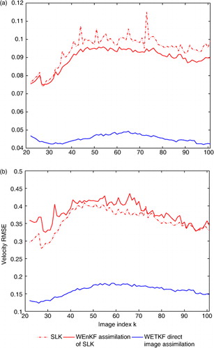
Fig. 2.  Synthetic 2-D turbulent flow. (a) Energy spectra; (b) error energy spectra.

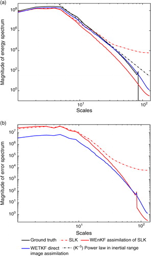
In addition to global error comparisons, the analysis of spectra plotted on Fig. 2 allows a more precise observation of the accuracy of the different techniques at different scales. Indeed, the RMSE constitutes only a performance measure at large scales. It is interesting to note that all methods only give relatively coherent results from the large scales up to the beginning of the inertial range. On the other hand, the result obtained with the WETKF assimilation scheme is closer to the ground truth over the whole scale range (from the largest scales up to the small dissipative scales). Again, this comes from the fact that this technique can benefit from all the available information in the image data, while pseudo-observations given by a local motion estimator will not improve the estimation at all-scales. Filters based on pseudo-observations are unable to correct the loss of energy caused by the smoothing operator used in the external estimation procedure.

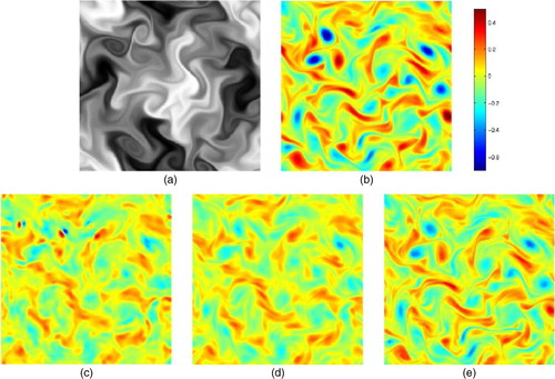
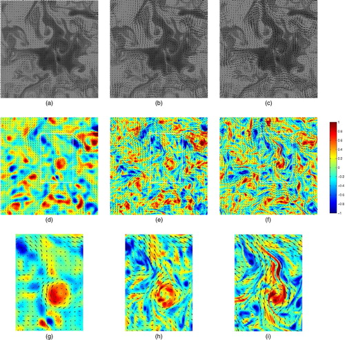
For a qualitative visual comparison, estimated vorticity maps are plotted on Fig. 3 at a given time instant. The scalar image observation is first presented, together with the ground truth vorticity on Fig. 3b. Figure 3c shows the vorticity estimated with the local SLK technique. The result obtained with the WEnKF assimilation scheme based on these SLK observations is presented on Fig. 3d, while Fig. 3e shows the result obtained with the proposed WETKF technique, assimilating image data directly. As can be seen on Fig. 3c, the vorticity estimated by the local motion estimation technique is far from the ground truth. As a consequence, the WEnKF assimilation based on these measurements only brings a small improvement since these observations do not carry enough information. The solution clearly lacks of energy compared to the true vorticity. The direct assimilation of image data through the WETKF scheme leads to a better estimation of vorticity structures, and in particular small scales structures as discussed previously with the comparison of spectra.

Fig. 3.  Synthetic 2-D turbulent flow. (a) Example of scalar image of the sequence at given time k; (b) ground truth vorticity at time k; (c) SLK vorticity estimate; (c) mean estimate of vorticity with WEnKF assimilation of SLK observation; (d) mean estimate of vorticity with WETKF direct assimilation of image data.

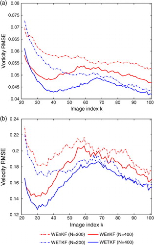
To conclude, the improvement obtained with the WETKF technique comes not only from the direct introduction of image data within the assimilation system, but also from the chosen ETKF strategy for the ensemble Kalman step. We highlight this improvement in Fig. 4, comparing the image assimilation technique with the ETKF scheme and standard EnKF scheme where the linear observation operator Hx _k is replaced by H(x _k ) as described in Section 2.2 eq. (8–8a) for the ETKF approach. Figure 4 shows that the best results are obtained with the ETKF scheme, for different sample sizes.

Fig. 4.  Comparison of WEnKF and WETKF techniques for the direct assimilation of image data. (a) RMSE between mean estimate of vorticity and ground truth; (b) RMSE between mean estimate of velocity and ground truth.

On this benchmark, we also compared in terms of vorticity the results obtained by WETKF and a similar ETKF version (non-weighted implementation of the filter). The results corresponding to different amounts of ensemble members are gathered in Table 1. These results correspond to the average mean–square error obtained over the last 20 images of the sequence and 10 realisations. The table shows the root mean–square vorticity error associated to the empirical mean and the mean–square dispersion of the ensemble around the ground truth (i.e. ). It can be observed that the results for ETKF and WETKF remain of the same order. The first moment and the ensemble dispersion are slightly lower for the weighted version. However, it is important to outline that RMSE constitutes only a large-scale criterion. To draw finer conclusions it is interesting to observe the error power spectrum (i.e. spectrum of the difference between the reference and the results averaged on the last 20 images and 10 realisations). These curves are plotted in Fig. 5a in log-k×spectrum for different number of particles. This graph depicts the amount of energy of the velocity error (w _err=w–w _ref) for each frequency band. For comparison purposes the ground truth spectrum and these curves are reproduced in the inside box graph. The error energy curves obtained by ETKF are plotted in dotted lines whereas those corresponding to WETKF are in a plain line. It can be noticed that for both methods and for the different number of particles the error energy is mainly concentrated within a frequency band corresponding to 80 to 8 pixels and the error energy bump inside this range decreases significantly when the number of particles increases. The results obtained with 10 particles have much higher error energy than for the other amount of particles and are not acceptable. There are clearly a limited number of particles below which errors are too important. For 50 particles WETKF provides lower errors on almost the whole frequency range the most part of the energy concentrates on. Another point of view can be obtained from the error power spectrum in log-log scale normalised by the ground truth power spectrum. This is shown in Fig. 5b. As can be observed for 10 particles, there is no scale range for which the normalised error energy drops below 10%. For 50 particles this 10% error-limit scale corresponds to 40 pixels. For 400 particles this scale reaches 25 pixels. Hence for both methods, low energy error levels are only obtained at coarse scales and accurate results at fine resolution requires significant augmentation of the particles. For a weak number of particles WETKF seems to perform slightly better than ETKF whereas for a higher number of particles both filters provide very similar results.

Fig. 5.  (a) Error Energy spectrum in log k vs. kE(k) scale obtained with ETKF (dotted lines) and WETKF (plain lines) for different number of particles; (b) Energy spectrum in log-log scale obtained with ETKF (dotted lines) and WETKF (plain lines) for different number of particles; (c) vorticity root-mean-square error along time obtained for WETKF with a diagonal constant observation variance (blue) and with the empirical image based variance (red).

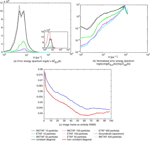
Table 1. Experiments on 2-D turbulence

Number of members	WETKF	ETKF
Results (mean estimation)
10	0.145	0.146
50	0.079	0.083
150	0.051	0.052
400	0.043	0.044
Results (ensemble dispersion)
10	0.146	0.147
50	0.080	0.084
150	0.053	0.053
400	0.045	0.046

Results obtained from WEKF and ETKF are compared. For both filters the dynamic's noise has a standard deviation of 0.01 and the parameters of the self-similar power law are fixed from the ground truth data. Mean-square estimation errors with respect to the ground truth and the ensemble dispersion around the ground truth are indicated in the table. Note the ground truth is associated to a zero variance as it is a deterministic system. The mean has been computed through an empirical average over the 20 last image frames of 10 realisations.

Figure 6 depicts the spatial maps of the second order moment. For both methods the evolution of this moment is plotted. We can observe that WETKF provides a faster method for a smoother variance map and ETKF shows at some localised places a higher variance. The ensemble covariance values for the centre line is also pictured in Fig. 7 (for 50 ensemble members) for WETKF and ETKF. Both techniques provide comparable results in terms of covariance length scale (around 15 pixels).

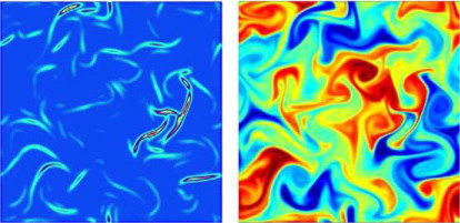
Lastly on this sequence, we plot in Fig. 8 as an example of the image-based observation variance, eq. (18). It is interesting to see that high variance value concentrates on thin structures corresponding to high photometric gradients. For this observation covariance, and 400 particles, we plot the evolution of the root mean-square error. We notice this parameter-free covariance observation model yields a better result than the previous constant variance.

Fig. 7.  Visualisation (with 50 members) of the covariance matrix values corresponding to the central line at t=99 left: ETKF, right: WETKF. The significative covariance length-scale is about 15×Δx large for both filters.

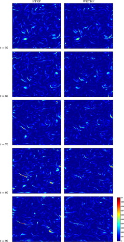
Fig. 8.  Left: visualisation for WETKF (with 400 members) of an example of the image-based adapted variance map associated to the displaced frame observation model; right: corresponding image of the passive scalar. High values of the standard deviation correspond to areas associated with high photometric gradient.

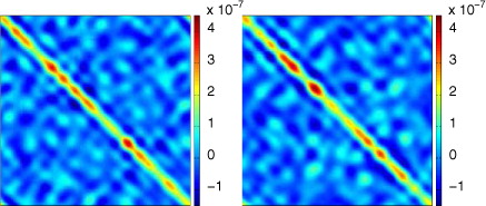
Fig. 6.  Example of the ensemble dispersion maps evolution along time; left column ETKF ensemble dispersion; right column WETKF ensemble dispersion.

The results described in this section comfort us on the use of the WETKF. The weight-updating step and the resampling are not computationally expensive and strengthen the robustness of EnKF for a relatively low number of particles. In the following sections, we will rely uniquely on such filters.

4.2. Results on real 2-D turbulence

The next set of experiments corresponds to real experimental images of a passive scalar transported by a turbulent flow. This image sequence corresponds to the experiments described in Jullien et al. (2000). The size of images is 512×512, and WEnKF and WETKF results have been obtained with N=300 particles. Vorticity results at a given time instant are plotted on Fig. 9 for the SLK technique, and both WEnKF (assimilating SLK results) and WETKF (assimilating image data). We note that the SLK motion estimation technique captures only coarse-scale vortices. The scales are successfully refined with the WEnKF assimilation relying on the same measurement and with the WETKF assimilation incorporating directly the non-linear image reconstruction error. The WETKF image assimilation reveals small motion scales exhibiting vortex filaments or stretching areas, which are smoothed out by SLK and WEnKF methods. This can be observed in inside the white delimited area of Fig. 9d–f, zoomed in on Fig. 9g–i. It must be pointed out that for the three techniques the estimated motion fields are quite close at large scale, so the results are consistent although based on different measurement operators. This might help validating these results, even if the ground truth is unknown here.

Fig. 9.  Real 2-D turbulent flow (Jullien et al., 2000). (a) Image at given time k and estimated velocity field with SLK; (b) image at given time k and estimated velocity field with WEnKF assimilation of SLK result; (c) image at given time k and estimated velocity field with WETKF direct assimilation of image data; (d) vorticity estimate with SLK and associated velocity field; (e) mean estimate of vorticity with WEnKF assimilation of SLK observation, and associated velocity field; (f) mean estimate of vorticity with WETKF direct assimilation of image data, and associated velocity field; (g–i) zoom in on white delimited areas of (d–f).

4.3. Results on oceanic data

Our final set of results concerns the application of the proposed WETKF technique on satellite images of SST, with large areas of missing data due to the cloud cover and presence of coastal regions.

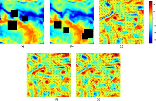
First of all, in order to highlight the capability of the method to cope with missing data, it is tested on a synthetic oceanic sequence. This sequence has been built from an initial real world 200×200 SST image transported by a synthetic flow, and respects the brightness consistency assumption given by eq. (17). The synthetic flow is the same 2-D turbulent flow as the one used in Section 4.1. Along the whole sequence, four square holes with side 20–45 pixels have been added randomly on each image. Figure 10 shows an example at a given time k of the sequence. Figures 10a and 10b show two consecutive images of the sequence, with the corresponding simulated ground truth velocity and vorticity on Fig. 10c. The result obtained with the WETKF assimilation scheme is presented on Fig. 10d from the images without missing data, and on Fig. 10e for the images with holes. It can be observed that the vorticity and velocity fields are estimated accurately, even in the presence of missing data. As a matter of fact, since for such regions the method relies on the dynamical model or on neighbourhood estimates, the spatiotemporal consistency is maintained. The results can be compared on Fig. 11 in terms of global RMSE between the mean estimates and the ground truth at each time step. The accuracy of the estimation deteriorates with missing data, but the error level remains low and stable with time.

Fig. 10.  Synthetic oceanic sequence with missing data. (a) Image at given time k; (b) image at given time k+1; (c) Ground truth vorticity and velocity field; (d) mean estimate of vorticity and velocity from WETKF assimilation of images without missing data; (e) mean estimate of vorticity and velocity from WETKF assimilation of images with missing data shown in (a) and (b).

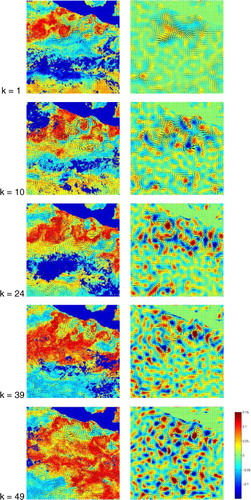
The method is then tested on a real oceanic sequence of SST images. The sequence consists of 48 images of size 256×256. The images have a spatial resolution of 0.1 degree (10 km) and a temporal period of 24 hours. The sequence is centred on an area of the Pacific Ocean off the Panama isthmus and shot during an El Niño episode. Representative results at different time instants of the sequence are shown in Fig. 12. The first column of Fig. 12 shows the estimated velocity fields at times k=1, 10, 24 and k=39, superimposed on the corresponding SST images. The second column shows the estimated vorticity maps and velocity fields. The initialisation for image 1 is based on the estimation provided by the local motion estimation approach (SLK). We see that this initialisation provides only a rough large-scale motion field. This estimate is refined afterward by the filtering process. We can note that the motion fields estimated along the sequence stick quite well to the big image structures observed on the SST images. The sequence of motion fields does not seem to be perturbed by the big missing data regions observed intermittently. Finally, we can note that the result obtained shows well an increase of the turbulent agitation with an intensification of the El-Niño phenomenon.

Fig. 11.  Synthetic oceanic sequence with missing data. (a) RMSE between mean estimate of vorticity and ground truth; (b) RMSE between mean estimate of velocity and ground truth.

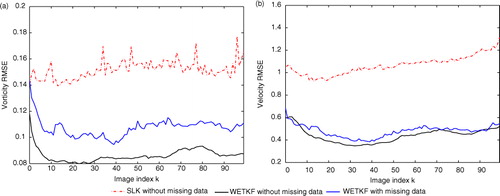
Fig. 12.  Real satellite sequence of SST (sea surface temperature) images. Dark blue regions indicate missing data due to the cloud cover or land regions. First column: SST images at different times k=1, 10, 24, 39, 49 and estimated velocity fields with the WETKF assimilation of image data. Second column: Mean estimated vorticity with WETKF and associated velocity fields.

Let us note there seems to be a good adequation between the 2-D vorticity dynamics used here and the data model based on (local in time) conservation of the observed quantity (the SST). This coupling enables extracting a 2-D component explaining the image observation deformation, which is consistent with a 2-D flow. The incorporation of more realistic 3-D oceanic models would require more a advanced data model allowing explaining luminance variations in a consistent way with respect to the dynamical models. In that prospect, the elaboration of data models relying on physical conservation laws might be of interest (Heitz et al., 2010).

5. Conclusion and discussion

In the context of image data assimilation, this study extends to mean-preserving square-root filters (Wang et al., 2004) – the weighted ensemble strategy proposed in Papadakis et al. (2010). This technique is defined as a particle filter in which the state variable trajectories sampling mechanism (i.e. the proposal distribution) is defined from an EnKF. This type of proposal function turned out to be experimentally much more efficient than the traditional sequential importance sampling based on the dynamics alone. Furthermore, compared to an importance sampling based on perturbed observations, a mean-preserving square-root filter sampling has shown to be more efficient for high-dimensional state space and a highly non-linear observation equation. A significant improvement was brought by this non-linear observation over velocity and uncertainty measurements provided by local motion estimation techniques (Corpetti and Mémin, 2012). Pseudo-observation of flow velocities constructed from local motion estimator techniques such as the Lucas and Kanade estimator (Lucas and Kanade, 1981) corresponds to measurements at too coarse scales. These measurements should not be used in image-based data assimilation. As those estimators have generally better performances than correlation techniques on scalar images (such as top of cloud pressure, SST, sea colour, etc.) the same conclusion applies also to maximum cross-correlation or particle image velocimetry techniques.

The non-linear reconstruction error based on the displaced frame difference criterion provide much better results. This criterion relies on a noisy transport assumption from frame to frame. This transport assumption is, however, only local since it applies just on the time interval in-between two images. It is thus a weaker assumption than the strong transport hypothesis over the whole assimilation window used in Titaud et al. (2010). Besides it enables when coupled with ensemble techniques to access to empirical observation error covariance that can easily be adapted to missing information regions. This ability has allowed us to apply such an assimilation on a real noisy sequence of SST. The results obtained for a simple 2-D velocity–vorticity formulation of Navier–Stokes (with stochastic forcing) are very promising and demonstrate the possibility to estimate a coherent velocity fields sequence from difficult images exhibiting poor photometric contrast and large regions with missing data. In future works, we plan to extend such an image-based assimilation strategy to more realistic geophysical models in oceanography or meteorology.

6. Acknowledgments

The authors thank the INRIA-Microsoft joint centre, and the ANR projects PREVASSEMBLE (ANR-08-COSI-012) and Geo-Fluids (ANR-09-SYSC-005) for their financial support. They acknowledge also the Ifremer CERSAT for providing them the oceanic SST image sequence.

Notes

¹Other solutions have been proposed to deal with non-Gaussianity in the framework of variational methods or stochastic filters [interested readers may refer to the review of Bocquet et al. (2010) or Yang et al. (2012)].

References

- Adrian R. Particle imaging techniques for experimental fluid mechanics. Annal Rev. Fluid Mech. 1991; 23: 261–304. 10.3402/tellusa.v65i0.18803.
- Anderson B. Moore J. Optimal Filtering. Prentice Hall, Englewood Cliffs, NJ.1979
- Anderson J. Anderson S. A Monte Carlo implementation of the nonlinear filtering problem to produce ensemble assimilations and forecasts. Mon. Weather Rev. 1999; 127(12): 2741–2758.
- Bishop C. Etherton B. Majumdar S. Adaptive sampling with the ensemble transform Kalman filter. Part I: Theoretical aspects. Mon. Weather Rev. 2001; 129(3): 420–436.
- Bocquet M. Pires C. Wu L. Beyond gaussian statistical modeling in geophysical data assimilation. Mon. Weather Rev. 2010; 138: 2997–3023. 10.3402/tellusa.v65i0.18803.
- Corpetti T. Héas P. Mémin E. Papadakis N. Pressure image asimilation for atmospheric motion estimation. Tellus A. 2009; 61: 160–178. 10.3402/tellusa.v65i0.18803.
- Corpetti T. Mémin E. Stochastic uncertainty models for the luminance consistency assumption. IEEE Trans. Image Process. 2012; 21(2): 481–493. 10.3402/tellusa.v65i0.18803.
- Del Moral P. Feynman-Kac Formulae Genealogical and Interacting Particle Systems with Applications. Springer, New York.2004
- Doucet A. Godsill S. Andrieu C. On sequential Monte Carlo sampling methods for Bayesian filtering. Stat. Comput. 2000; 10(3): 197–208. 10.3402/tellusa.v65i0.18803.
- Elliot F. Horntrop D. Majda A. A Fourier-wavelet Monte Carlo method for fractal random fields. J. Comput. Phys. 1997; 132(2): 384–408. 10.3402/tellusa.v65i0.18803.
- Emery W. Thomas A. Collins M. Crawford W. Mackas D. An objective method for computing advective surface velocities from sequential infrared satellite images. J. Geophys. Res. 1986; 91: 12865–12878. 10.3402/tellusa.v65i0.18803.
- Evensen G. Sequential data assimilation with a non linear quasi-geostrophic model using Monte Carlo methods to forecast error statistics. J. Geophys. Res. 1994; 99(10): 143–162.
- Evensen G. The ensemble Kalman filter, theoretical formulation and practical implementation. Ocean Dynam. 2003; 53(4): 343–367. 10.3402/tellusa.v65i0.18803.
- Gordon, N, Salmond, D and Smith, A. 1993. Novel approach to non-linear/non-gaussian bayesian state estimation. IEEE Processing-F. 140(2).
- Heitz D. Memin E. Schnoerr C. Variational fluid flow measurements from image sequences: synopsis and perspectives. Exp. in Fluids. 2010; 48(3): 369–393. 10.3402/tellusa.v65i0.18803.
- Houtekamer P. Mitchell H. A sequential ensemble Kalman filter for atmospheric data assimilation. Mon. Weather Rev. 2001; 129(1): 123–137.
- Houtekamer P. L. Mitchell H. Data assimilation using an ensemble Kalman filter technique. Mon. Weather Rev. 1998; 126(3): 796–811.
- Hunt B. Kostelich E. ISzunyogh I. Efficient data assimilation for spatiotemporal chaos: A local ensemble transform Kalman filter. Physica D. 2007; 230: 112–126. 10.3402/tellusa.v65i0.18803.
- Jullien M.-C. Castiglione P. Tabeling P. Experimental observation of batchelor dispersion of passive tracers. Phys. Rev. Lett. 2000; 85: 3636–3639. 10.3402/tellusa.v65i0.18803.
- Kalman R. A new approach to linear filtering and prediction problems. Tans ASME – J. Bas. Eng. 1960; 82: 35–45. 10.3402/tellusa.v65i0.18803.
- Kloeden P. Platen E. Numerical Solution of Stochastic Differential Equations. Springer, Berlin.1999
- Kraichnan, R. 1968. Small-scale structure of a randomly advected passive scalar. Phys. Rev. Lett. 11, 945–963.
- Lauritzen S. Graphical Models. Oxford University Press, Oxford, UK.1996
- Le Dimet F.-X. Navon I. Daescu D. Second-order information in data assimilation. Mon. Weather Rev. 2002; 130(3): 629–648.
- Lucas, B and Kanade, T. 1981. An iterative image registration technique with an application to stereovision. Int. Joint Conf. on Artificial Intel. 2, 674–679.
- Majda A. Kramer P. Simplified models for turbulent diffusion: theory, numerical modelling, and physical phenomena. Physics Report. 1999; 314: 237–574. 10.3402/tellusa.v65i0.18803.
- Ott, E, Hunt, B, Szunyogh, I, Zimin, A, Kostelich, M. C. E. J. and co-authors. 2004. A local ensemble Kalman filter for atmospheric data assimilation. Tellus A. 56, 415–428. 10.3402/tellusa.v65i0.18803.
- Ottenbacher A. Tomasini M. Holmund K. Schmetz J. Low-level cloud motion winds from Meteosat high-resolution visible imagery. Weather Forecast. 1997; 12(1): 175–184.
- Papadakis N. Mémin E. An optimal control technique for fluid motion estimation. SIAM J Imag Sci. 2008; 1(4): 343–363. 10.3402/tellusa.v65i0.18803.
- Papadakis N. Mémin E. Cuzol A. Gengembre N. Data assimilation with the weighted ensemble Kalman filter. Tellus A. 2010; 62(5): 673–697.
- Sakov P. Oke P. Implications of the form of the ensemble transformation in the ensemble square root filter. Mon. Weather Rev. 2007; 136: 1042–1053. 10.3402/tellusa.v65i0.18803.
- Shu, C.-W. 1998. Advanced Numerical Approximation of Nonlinear Hyperbolic Equations. Lecture Notes in Mathematics. Vol. 1697. Springer: Berlin/Heidelberg, 325–432.
- Snyder C. Bengtsson T. Bickel P. Anderson J. Obstacles to high-dimensional particle filtering. Mon. Weather Rev. 2008; 136(12): 4629–4640. 10.3402/tellusa.v65i0.18803.
- Souopgui, I, Dimet, F.-X. L and Vidard, A. 2009. Vector field regularization by generalized diffusion. Technical Report RR-6844. INRIA, Roquencourt, FRANCE.
- Szantai A. Desbois M. Désalmand F. A method for the construction of cloud trajectories from series of satellite images. Int. J. Remote Sens. 2002; 23(8): 1699–1732. 10.3402/tellusa.v65i0.18803.
- Thomas C. Corpetti T. Mémin E. Data assimilation for convective cells tracking on meteorological image sequences. IEEE Trans. Geosci Remote Sens. 2010; 48(8): 3162–3177. 10.3402/tellusa.v65i0.18803.
- Tippett M. Anderson J. Craig C. B. Hamill T. Whitaker J. Ensemble square root filters. Mon. Weather Rev. 2003; 131(7): 1485–1490.
- Titaud O. Vidard A. Souopgui I. Dimet F.-X. L. Assimilation of image sequences in numerical models. Tellus A. 2010; 62(1): 30–47. 10.3402/tellusa.v65i0.18803.
- Van Leeuwen, P. J. 2009. Particle filtering in geophysical systems. Mon. Weather Rev. 137.10.3402/tellusa.v65i0.18803.
- Wang X. Bishop C. Julier S. Which is better, an ensemble of positive-negative pairs or a centered simplex ensemble?. Mon. Weather Rev. 2004; 132: 1590–1605.
- Yang, S.-C, Kalnay, E and Hunt, B. 2012. Handling Nonlinearity in an Ensemble Kalman Filter: Experiments with the Three-Variable Lorenz Model. Mon. Wea. Rev. , 140, 2628–2646. 10.3402/tellusa.v65i0.18803.