What can we learn about climate feedbacks from short-term climate variations?

ABSTRACT

This study examines the radiative feedbacks resulting from changes in the climate over the last 30 yr. These ‘short-term’ feedbacks correspond to both external changes in the forcing [from greenhouse gases (GHGs), aerosols etc.] and internal climate variations [mostly due to El Niño Southern Oscillation (ENSO)]. They differ from the ‘long-term’ (century scale, mainly due to GHG warming) feedbacks both in magnitude (by 24% on the global average) and geographical distribution, according to the Coupled Model Intercomparison Project phase 3 multi-model dataset. In addition, the inter-model spread of the short-term feedbacks is larger than the long-term ones even for the models with the best ENSO performance, which indicates that important aspects of the ENSO variability are still poorly understood and/or simulated. Information from observations and from advanced reanalysis systems can be very useful to improve the model short-term climate responses. However, long and accurate observational records are critical in order to obtain confident results.

• feedbacks
• long-term
• ENSO
• climate change
• radiative kernels

1. Introduction

The response of the Earth's climate system to perturbations in the radiation budget due to changes in anthropogenic greenhouse gases (GHGs) is influenced by a number of internal processes, called the climate feedbacks (National Research Council, 2003). Such climate feedbacks constitute processes that respond to a change in global mean surface temperature and directly or indirectly affect the Earth's radiation budget (Bony et al., 2006). Here I focus on the ‘radiative’ feedbacks (i.e. those that directly affect the radiation budget through physical processes) via changes in water vapour, clouds, temperature and surface albedo.

Radiative feedbacks can be estimated using global climate models based on the difference between two climate states, a perturbed (e.g. doubled CO₂ concentration) versus a control climate state (usually defined at preindustrial or present conditions). However, this involves long integrations of global climate models, which require a substantial amount of computer time. A method that avoids long computations is the ‘radiative kernel’ method, which decomposes a feedback into two parts, one that depends on radiative transfer and the unperturbed climate state, and a second factor that arises from the climate response of the feedback variable (Shell et al., 2008; Soden et al., 2008). An overview of the different approaches used to quantify feedbacks, including the radiative kernel method, can be found in Chung et al. (2012).

Currently, global climate models disagree in their estimates of feedbacks and this is one of the main reasons for uncertainty in future climate projections (Bony et al., 2006). In order to unveil the origin of these inter-model differences, model simulations need to be evaluated against observations of present climate. Present-day climate feedbacks can be estimated based on the differences between climate states resulting either from short-term natural variability, such as the diurnal and seasonal variation, the land–ocean contrast, the El Niño Southern Oscillation (ENSO) variation and others, or from short-term external natural forcing, e.g. from volcanic aerosols. For example, Hall and Qu (2006) have used the current seasonal cycle to constraint snow albedo feedback under future climate change. Knutti et al. (2006) have found correlations between simulated seasonal cycle amplitudes and climate sensitivity in climate models in several regions. Several studies have tried to constrain climate sensitivity and feedbacks from ENSO-controlled fluctuations in satellite data (Forster and Gregory, 2006; Dessler et al., 2008; Murphy et al., 2009; Trenberth et al., 2010). More recently, Dessler (2010, 2012) has used the ‘radiative kernels’ method to estimate the global average feedbacks in response to changes in global surface temperature due to the ENSO not only from global climate models but also based on a combination of satellite and re-analysis data.

Short-term climate variations due to ENSO have been used to estimate feedbacks for a number of reasons. First, ENSO is a dominant mode of interannual variability in the Earth's climate system and has a substantial global impact through global atmospheric teleconnections. During El Niño, global mean surface temperature increases by several tenths of a degree, which unmasks the climate feedback signals above the natural climate variability. In addition, under global warming conditions models simulate a climate response in the tropics that resembles an El Niño response. However, the geographical structures of the surface temperature changes and the associated circulation responses due to ENSO variability are different from those under global warming (Bony et al., 2006; Zhu et al., 2007; Lu et al., 2008).

Second, global climate models have significantly improved over the last decade and now display, at least qualitatively, realistic ENSO behaviour (van Oldenborgh et al., 2005; Guilyardi et al., 2009). Nevertheless, they are still unable to simulate many features of ENSO variability and its circulation teleconnections, and these deficiencies are sometimes common to many models (Joseph and Nigam, 2005; van Oldenborgh et al., 2005; AchutaRao and Sperber, 2006; Reichler and Kim, 2008; Guilyardi et al., 2009).

Finally, over the past few decades, ENSO has been monitored quite extensively and observational (in situ and remote) data are currently available. However, a problem when dealing with short-term climate variations is the presence of natural ‘chaotic’ variability (weather), which contaminates the radiative feedback signal in such short period observations (Spencer and Braswell, 2011). Long-term datasets of at least a few decades are thus necessary in order to detect robust feedback signals.

In this study, I estimate the feedbacks from water vapour, lapse-rate, Planck, surface albedo and clouds, using models and observations based on the climate response over the last 30 yr. A significant amount of global warming occurred during this period (about 0.5°C based on data from http://data.giss.nasa.gov/gistemp/), and therefore these ‘short-term’ feedbacks result both from external changes in the forcing (due to GHG increases, volcanic and industrial aerosol emissions) and internal climate variations (mostly due to ENSO variability). I investigate the regions with the largest uncertainties between the models in comparison to those computed based on the ‘long-term’ (century long) GHG changes and in comparison to estimates from recent satellite and reanalysis data. In particular, the aim of this study is to address the following questions:

• Where and why global climate models diverge in respect to their short-term climate responses?

• How can we use models and observations to better understand climate feedbacks?

In Section 2, I present a brief definition of feedbacks used in this study. Section 3 describes the data and methods used to estimate feedbacks. Section 4 compares the magnitudes and geographical distributions of the long-term and short-term climate feedbacks. Sections 5 and 6 discuss the uncertainty in model results based on the inter-model spread and in comparison to reanalysis data, respectively. I summarize the major points of this study in Section 7.

2. Definition of radiative feedbacks

To first order, the radiative forcing ΔQ (Wm⁻²) can be related through a linear relationship to the global average temperature change ΔT _s at the surface (K) and the radiative imbalance at the top of the atmosphere (TOA) ΔR (Wm⁻²), as follows (the overbar indicates global averaging):1

The parameter λ in equation (1) is called the climate feedback parameter (Wm⁻²K⁻¹) and represents the enhanced emission of energy to space as the planet warms (λ is therefore a negative number).

In our definition, rapid stratospheric adjustments are included in the forcing but rapid tropospheric adjustments are included in the feedbacks. Recent studies have shown that the tropospheric adjustments occur with instantaneous large increase in CO₂ forcing primarily through cloud changes (Andrews and Forster, 2008; Gregory and Webb, 2008; Williams et al., 2008) and that it should be considered as part of the forcing. However, an instantaneous large step increase in CO₂ forcing does not occur in the real word and thus, further work is needed in order to examine whether such adjustments are realized at smaller magnitude forcings such as in transient forcing scenarios (Andrews et al., 2011).

Following Bony et al. (2006), climate feedback constitutes any process that responds to a change in global mean surface temperature and directly or indirectly affects the Earth's radiation budget. Feedbacks therefore represent internal processes of the system. Let x _i represent a climate variable affecting R, the feedback parameter λ, can be defined as follows:2

In equation (2), I assume that the feedbacks are independent and so they can be added together. Positive (negative) values of feedbacks and forcings denote an energy gain (loss) for the system, respectively. The climate feedback parameter λ contains the Planck response λ ₀, as well as the climate feedbacks (λ _i). The Planck (or basic) response is the most fundamental response in the climate system owing to the temperature dependence of radiative emission through the Stefan-Boltzmann law of blackbody emission. This is the most important restoring term producing a stable climate (i.e. making λ negative). Here, I focus on the fast radiative feedbacks associated with the interaction of the Earth's radiation budget with water vapour, clouds, temperature and surface albedo in snow and sea ice regions (λ=λ _q+λ _c+λ _T+λ _a), respectively. The temperature feedback (λ _T) can be decomposed to its two components, the lapse rate feedback (λ _lr) and the Planck response λ ₀, assuming that the surface temperature changes are vertically homogeneous in the troposphere. Notice that this definition of λ ₀ does not correspond exactly to a vertically and horizontally uniform temperature change but is common in GCM calculations (see Appendix in Bony et al., 2006). Feedbacks due to changes in the biosphere, in trace gases and aerosols, in the ice sheets or in the deep ocean are not considered in this study, even though they might have a substantial impact on the magnitude, the pattern, or the timing of climate warming (Bony et al., 2006).

3. Data and methods

Feedbacks are computed from the multi-model dataset of the World Climate Research Programme's (WCRP's) Coupled Model Intercomparison Project phase 3 (CMIP3) (Meehl et al., 2007a). I used two types of experiments, the ‘Climate of the 20th Century’ or ‘20C3M’ and the ‘720 ppm stabilization’ or ‘A1B scenario’ (Nakićenović et al., 2000). There are 13 models (Table 1) with all the necessary data available for the computations (temperature, specific humidity, surface albedo, all sky and clear sky TOA radiation fluxes). I also calculate feedbacks utilizing reanalysis data from the European Centre for Medium-Range Weather Forecasts (ECMWF) ERA-Interim (Dee et al., 2011) and the Japanese 25-year Reanalysis Project (JRA-25) (Onogi et al., 2007). The reanalyses data are available for the period from 1979 to 2009 (31 yr).

Table 1. List of the CMIP3 models used in this study. The models with asterisk in their name have included volcanic forcing in their 20C3M experiments

Number	Model name	Originating group	Country
1	ccma_cgcm3_1	Canadian Centre for Climate Modeling and Analysis	Canada
2	cnrm_cm3	Centre National de Recherches Météorologiques (Météo France)	France
3	gfdl_cm2_0*	Geophysical Fluid Dynamics Laboratory (NOAA)	USA
4	gfdl_cm2_1*	Geophysical Fluid Dynamics Laboratory (NOAA)	USA
5	giss_model_e_h*	Goddard Institute for Space Studies (NASA)	USA
6	giss_model_e_r*	Goddard Institute for Space Studies (NASA)	USA
7	inmcm3_0*	Institute of Numerical Mathematics	Russia
8	ispl_cm4	Institut Pierre Simon Laplace	France
9	miroc3_2_hires*	Center for Climate System Research	Japan
10	miroc3_2_medres*	Center for Climate System Research	Japan
11	mpi_echam5	Max Planck Institute for Meteorology	Germany
12	mri_cgcm2_3_2a*	Meteorological Research Institute	Japan
13	ncar_ccsm3_0*	National Center for Atmospheric Research	USA

For the cloud feedback computation, in particular, I combine the reanalysis with satellite data following Dessler (2010) as discussed in details below. I use the all-sky TOA energy flows of the Energy Balanced and Filled (EBAF) data product of the Clouds and Earth's Radiant Energy System (CERES) satellite instruments (Loeb et al., 2009).

I use the radiative kernel method (Soden et al., 2008) to compute the feedbacks, which facilitates the understanding of the causes of differences among models or between models and observations, since the differences arise from the actual climate response of the feedback variables and not from differences in their radiative transfer code (Chung et al., 2012). More precisely, this method computes the feedbacks as a product of two terms: (a) the climate response of climate variables (in this case, temperature, water vapour and surface albedo) to an imposed forcing; and (b) the radiative kernels which describe the radiative effects of these climate variable changes. Both the kernel and the response for each climate variable are functions of latitude, longitude, altitude and month. Each λ _i is vertically integrated from the surface to the tropopause and globally averaged to yield global feedback parameters (for details on the method see Soden et al., 2008). Radiative kernels are similar for different models (Soden et al., 2008) and therefore a single model kernel can be used to estimate feedbacks for any model simulation. The results of this study are based on the GFDL radiative kernels described in Soden et al. (2008).

The response is computed for each model as follows: The long-term climate change response is determined by the difference in temperature, water vapour, surface albedo and global mean surface temperature between global model simulations of future-climate (average over the period 2101–2130 from the A1B experiments) versus present-day conditions (average over 1970–2000 from the 20C3M experiments). The response due to short-term interannual climate variations is computed from the slope of the linear least squares fit between the monthly anomalies in temperature, water vapour and surface albedo and the monthly anomalies in global mean surface temperature. The model responses are computed from 30-yr period (1970–2000) anomalies of the coupled model 20C3 experiments. For the reanalyses data, the short-term responses are computed in the same way but for the period from 1979 to 2009. The climate feedbacks for each variable derive from the product of the above climate responses with the three-dimensional kernels from the GFDL model.

Due to non-linearities, the cloud feedback is not computed with the kernel method, but estimated from the change in the cloud radiative forcing (ΔCRF) (i.e. cloudy sky minus clear-sky TOA net fluxes) after adjusting for the effects of the changes in the non-cloud (i.e., T, q and a) variables, following Soden et al. (2008):3

This method also requires information on forcing changes under cloudy-sky (ΔQ) and clear sky (ΔQ ⁰) conditions, which is not available in the models output. In addition, the radiative forcings imposed in both the 20th century and future scenario simulations vary from model to model mainly due to the incorporation of aerosols for some of the models (see Table 10.1 in Meehl et al., 2007b), and due to the inter-model differences in their emissions, physical processes and radiative effects. For example, 7 out of 13 models of this study prescribed time-varying black carbon aerosols in their simulations, while in the rest of the models their concentrations remain constant with time. Furthermore, the inter-model differences in the aerosol forcing may induce differences in the spatial pattern of surface temperature changes between models, thereby causing inter-model differences in other climate feedbacks, as well. Nevertheless, due to the lack of information of aerosol forcing changes, I do not take it into account in the cloud feedback calculation. Given the important inter-model differences in aerosol changes and their radiative impact, not taking aerosol forcing into account likely contributes to the inter-model spread of feedbacks and should not introduce a bias (Previdi, 2010).

In the case of well-mixed GHGs, all models prescribed the same changes in their concentrations. For the long-term cloud feedback calculation, the change in the all-sky GHG forcing (ΔQ=Q ^{(2101–2130)}−Q ^{(1970–2000)}) is equal to 4.3 Wm⁻², based on the annual IPCC GHGs concentrations converted using the Myhre et al. (1998) simplistic equations. Following Soden et al. (2008), I assume that the cloud masking reduces the global average radiative forcing by ~16% (i.e. (ΔQ ⁰–ΔQ)/ΔQ), as estimated based on the GFDL radiation code. Therefore, the resulting (ΔQ ⁰–ΔQ) is equal to 0.69 Wm⁻².

An additional complexity in the case of short-term cloud feedbacks arises from the requirement for information on the seasonal variation of the forcing. The monthly GHG forcing (ΔQ) is computed by linearly interpolating the annual means (computed in a similar way as before from the IPCC GHG concentrations) for the given study period (1970–2000). For those models that include changes in the volcanic forcing in their 20C3M experiments (see Table 1), I use the global-average monthly volcanic forcing estimates based on Sato et al. (1993). As stated previously, not taking aerosol forcing in the cloud feedback computation into account should aggravate the inter-model spread but should not introduce a bias.

The short-term cloud forcing is computed in a similar way as in the models, except the ΔCRF is determined by subtracting the TOA net flux obtained by the CERES instruments, from the TOA net flux at clear-sky conditions obtained from the re-analyses, following Dessler (2010). The cloud feedback is therefore computed based on a shorter period (10 yr) when the CERES data are available (2001–2009). Following Dessler (2010), I also add ±0.18 Wm⁻²K⁻¹ uncertainty in the cloud feedback in order to account for the impact of spurious long-term trends in the CERES data.

4. Long-term versus short-term climate feedbacks

In this section, I compare the climate feedbacks computed from the CMIP3 models and based on long-term or short-term changes. I focus on the CMIP3 multi-model mean, which has been shown to outperform any single model due to compensating systematic errors (Glecker et al., 2008; Pincus et al., 2008; Reichler and Kim, 2008; Knutti et al., 2010). The magnitudes of the calculated feedbacks are not significantly different than the ensemble mean even if using only a small subset of three models (4: gfdl_cm2_1, 9: miroc3_2_hires, 11: mpi_echam5) with the most reliable ENSO representation according to van Oldenborgh et al. (2005). The average global feedback strengths are shown in Table 2 (individual model results are available in Tables A.1 and A.2 of Appendix). The confidence intervals for the short-term feedbacks represent the two standard deviations (±2σ) in the regression analysis and not the inter-model range, the latter being discussed in detail in Section 5.

Table 2. Global average CMIP3 multi-model mean (MM) feedbacks and interdecile range (IDR: the difference between the 90th and the 10th percentile of the model estimates) calculated based on long-term and short-term climate variability (see text for details). Results are also shown for the ERA-Interim, JRA-25 re-analyses. For the short-term feedbacks, the 2σ least squares fit uncertainty is indicated, as well. Units are Wm²K⁻¹

	Planck response	Lapse rate	Water vapour	Surface albedo	Cloud	Net
a) Long-term
CMIP3 MM (2101–2130) vs (1970–2000)	−3.24	−0.84	1.88	0.27	0.56	−1.36
IDR	0.09	0.72	0.51	0.21	1.04	1.06
b) Short-term
CMIP3 MM±2σ ‘20C’ (1970–2000)	−3.18±0.04	−0.58±0.19	1.78±0.15	0.22±0.06	0.73±0.30	−1.03±0.39
IDR	0.19	1.07	1.11	0.38	1.36	1.46
ERA-Interim (1979–2009)	−2.96±0.04	0.11±0.16	0.86±0.14	0.12±0.04	0.33±0.82*	−1.54±0.85
JRA-25 (1979–2009)	−3.15±0.04	0.34±0.20	1.37±0.16	0.20±0.06	0.86±1.10*	−0.38±1.13

*Calculated over the period 2001–2009.

4.1. Planck response

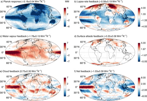
The Planck response, λ ₀ provides a measure of the geographical distribution of surface temperature changes, which is useful for understanding the differences between short and long-term feedbacks, as discussed in the following. Figures 1a and 2a show the spatial variation of the Planck response for the CMIP3 multi-model mean based on long-term and short-term changes, respectively. In both cases, the Planck response shows negative values almost everywhere (i.e. temperature increase) and especially over land areas, where the warming is largest. The large sea surface temperature variation in the eastern and central equatorial Pacific during ENSO is reflected in the stronger response over this region in the case of the short-term Planck response. Larger (more negative) values are found in the high latitude land areas in the northern hemisphere, while lower values occur in the northern and southern mid-latitudes (between 30° and 60°) in comparison to the long-term GHG response, which, as expected, is globally more uniformly distributed. Despite the differences in their geographical patterns, the long-term and short-term global average feedbacks differ only by a few percent (−3.24 and −3.18±0.04 Wm⁻²K⁻¹, respectively).

Fig. 1.  Global maps of all the radiative feedbacks (Planck, lapse rate, water vapour, surface albedo, cloud and net) of the CMIP3 multi-model mean, calculated based on their response from long-term climate changes due to the increase in greenhouse gas forcing. Units are in Wm⁻²K⁻¹.

4.2. Lapse-rate feedback

The CMIP3 models predict enhanced warming in the upper troposphere of tropical regions in response to an increase in the GHGs, which leads to reduced rate of temperature decrease with height, and thus, a negative lapse rate feedback (−0.84 Wm⁻²K⁻¹, see Fig. 1b). On the contrary, at mid- to high-latitudes and, especially over land areas, more low-level warming is projected providing a positive lapse-rate feedback (Goose et al., 2010). The short-term simulated lapse-rate response (Fig. 2b) shows similar geographical structure (positive values at the high latitudes over land and negative values in most of the tropics), apart from a positive lapse-rate feedback in the tropical Pacific Ocean, which is related to the larger upper ocean warming during El Niño conditions. The short-term feedback is also larger in the northern mid and high latitude land areas associated with larger surface temperature changes during El Niño, as also shown for the Planck response. As a result, the global average multi-model mean lapse rate feedback is ~35% larger (−0.58±0.19 Wm⁻²K⁻¹) if computed based on short-term variability in comparison to long-term change (−0.84 Wm⁻²K⁻¹).

Fig. 2.  Global maps of all the radiative feedbacks of the CMIP3 multi-model mean calculated based on their response from short-term climate variability. Units are in Wm⁻²K⁻¹.

4.3. Water vapour feedback

The water vapour feedback is found to be positive everywhere in the long-term experiments (Fig. 1c) following the Clausius-Clapeyron equation and a quasi-constant relative humidity. It is especially larger in the tropics due to large increases in specific humidity in the dry upper troposphere (Zelinka and Hartmann, 2011). The water vapour feedback inferred from short-term variations is even larger in the tropics, but lower in the subtropics and in mid- and high-latitude regions of negligible change in sea surface temperatures (SSTs). On average globally, the long-term water vapour feedback is however larger (1.88 Wm⁻²K⁻¹) than the short-term feedback (1.78±0.15 Wm⁻²K⁻¹).

In most of the GCMs, relative humidity changes little during both climate change and ENSO variability experiments (Held and Soden, 2006; Dessler and Sherwood, 2009). A warming of the tropical atmosphere is associated with a negative lapse-rate feedback and a positive upper-tropospheric water vapour feedback. Lapse-rate and water vapour feedbacks are therefore cancelling each other out and are often combined into a single feedback. The combined water vapour +lapse rate feedback is 1.04 Wm⁻²K⁻¹ and 1.2±0.24 Wm⁻²K⁻¹, based on long-term climate changes due to long-term and short-term climate variations, respectively.

4.4. Surface albedo feedback

The long-term surface albedo (or snow–ice) feedback is positive (0.27 Wm⁻²K⁻¹) and confined mostly to high latitudes as expected (Fig. 1d). This is also the case for the short-term surface albedo feedback (Fig. 2d) although it is somewhat lower (0.22±0.06 Wm⁻²K⁻¹) due to lower values especially in the northern part. The differences may reflect ENSO influences on the Arctic and Antarctic sea ice concentrations (e.g. Liu et al., 2004; Turner, 2004; Yuan, 2004), but the effect of ENSO in polar surface temperature varies greatly between the models (see also Section 5).

4.5. Cloud feedback

The multi-model mean cloud feedbacks for the long-term and short-term changes are shown in Figs. 1e and 2e. There are marked differences between them, with the long-term cloud feedback showing a latitudinal change from positive to negative values poleward of around 50°, while the short-term cloud feedback shows a much larger spatial variability (note also the two times larger colour scale). These differences can be better understood if one looks at the decomposed longwave (LW) and shortwave (SW) cloud components shown in Fig. 3.

Fig. 3.  Global maps of the long-term (left panels) and short-term (right panels) cloud (longwave, shortwave and net) feedbacks. Units are in Wm⁻²K⁻¹.

The long-term LW cloud feedback is positive in most regions and for almost all models reflecting the rise of clouds as climate warms (Zelinka et al., 2012). Concurring decreases in cloud amount however, reduces its magnitude by more than half (Zelinka et al., 2012). The larger LW cloud feedback values in the central equatorial pacific are related to increased cloud fraction, which results from the ‘El Niño-like’ pattern of anomalously high SSTs simulated by the models. The short-term LW cloud feedback shows a similar pattern in the equatorial pacific but of a larger magnitude driven by higher SST anomalies. In contrast to the long-term LW feedback, the short-term LW feedback over the subtropics and the tropical Atlantic Ocean show large negative values related to reductions in total cloud amount (see e.g. Klein et al., 1999).

The positive values of the modelled SW long-term cloud feedback equatorward 50° (Fig. 3c) are due to the decrease in cloud amount (Zelinka et al., 2012), except the large region in the central equatorial pacific where increases occur (and therefore a negative cloud SW feedback), as discussed previously. Changes in cloud fraction simulated from the CMIP3 models are responsible for the geographical pattern of the short-term SW cloud feedback as well, showing negative values in the tropical pacific due to increase in cloud amount, and positive values in the subtropics as a result from reductions in cloud amount. These are largely counteracted by the LW short-term cloud feedback pattern of the opposite sign. Consequently, the net (LW+SW) short-term cloud feedback varies less latitudinally, except in the tropical pacific where it shows positive values due to increased cloud amount (Fig. 3f).

Poleward of 50°, negative values of SW long-term cloud feedback are related to cloud fraction increases, associated with poleward-shifted storm tracks (e.g. Bengtsson et al., 2005; Yin, 2005) and with increased optical depth (brightening) of cold low clouds (Zelinka et al., 2012). Tropospheric zonal jets tend to move equatorward in response to El Niño (Bengtsson et al., 2005, Lu et al., 2008), but, despite the associated cloud fraction decrease, the SW short-term response on clouds is found to be either weak (in the NH) or negative (in the SH). This supports the argument by Zelinka et al. (2012) that the enhanced reflection is primarily due to the increase in cloud brightness at high latitudes related to changes in the phase and/or total water contents on clouds as temperature increases. Notice however, that the CMIP3 models were shown to have biases in cloud amount and cloud optical depth at mid latitude ocean domains, and especially over the Southern ocean and the change in cloud properties and feedbacks are likely to be dependent on such biases (Trenberth and Fasullo, 2010). Driven by the larger LW and SW cloud responses, the net cloud feedback computed from the short-term variations is larger than the long-term cloud feedback by 0.17 Wm²K⁻¹ or ~30% (0.73±0.29 in comparison to 0.56 Wm²K⁻¹, respectively).

4.6. Can we use present-climate short-term variations to constrain long-term climate feedbacks?

Despite the important regional differences between the long-term and short-term multi-model mean feedbacks, their global averaged values correspond within 30% according to the models, as also shown in Fig. 4. The greatest difference between the long-term and short-term feedbacks is found for the lapse-rate (0.26 Wm⁻²K⁻¹ or 31%) and cloud feedback (0.17 Wm⁻²K⁻¹ or 30%). However, due to error compensation, the combined water vapour-lapse rate feedback corresponds much better between the two methods (0.16 Wm⁻²K⁻¹ or 15%). The net feedbacks differ by about 24% (or 0.33 Wm⁻²K⁻¹) between the two methods according to the models.

Fig. 4.  Radiative feedbacks (Planck, water vapour, lapse-rate, the combined water vapour plus lapse-rate feedback, surface albedo, cloud and net), computed for each of the CMIP3 models (in grey) and the multi-model mean (in black) for the long-term climate change experiments. The CMIP3 models and multi-model mean feedbacks (and their 2σ confidence intervals) computed based on the short-term variations are denoted in pink and black dots, respectively. Results from the ERA-Interim and JRA-25 re-analyses are shown in blue and green, respectively. Units are in Wm⁻²K⁻¹.

However, it is important to realize that the models most likely underestimate the above differences. First, present day and future climate responses in the models are not independent from each other, since the latter are essentially based on our knowledge of the physical mechanisms observed in the last few decades. It is thus probable that the response of real climate under increased GHG forcing is driven by physical mechanisms that are not included in the current models. In addition, unrealistic physical relationships present in the models may introduce positive correlation between the long-term and short-term feedbacks. For example, surface albedo and cloud feedbacks are likely to be dependent on the present-day simulated amounts of ice and cloud, respectively (Boe et al., 2010; Trenberth and Fasullo, 2010), and this may have similar implications for both short-term and long-term changes. Caution therefore must be exercised when using short-term climate variability as a replacement in calculating long-term climate feedbacks.

5. Inter-model variability

Investigating differences amongst the models is useful in identifying the regions and possibly the processes with the largest uncertainties. Focusing on these processes and comparing them with present-day observations can help improve climate models and, thus, provide greater confidence in their future climate projections. Keep in mind, however, that models are not independent between them and, thus, processes where models tend to agree should not be interpreted as less uncertain (Huybers, 2010; Knutti et al., 2010). As a measure of the statistical dispersion between the model simulations, I calculate the interdecile range (IDR), which is the difference between the ninth and the first deciles (90% and 10%), at each model grid point and for each climate feedback. Results for both long-term and short-term climate feedbacks are shown in Figs. 5 and 6, respectively.

Fig. 5.  Global maps of the interdecile range of the CMIP3 models for the long-term feedbacks. Units are in Wm⁻²K⁻¹.

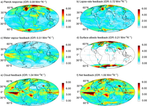
Fig. 6.  Global maps of the interdecile range of the CMIP3 models for the short-term feedbacks. Units are in Wm⁻²K⁻¹.

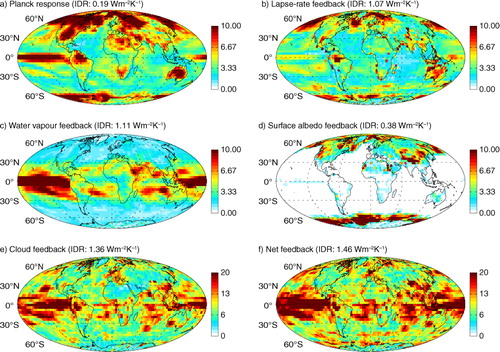
The first thing to note is that the inter-model spread is much larger for all short-term feedbacks in comparison to the long-term ones. The IDR for the short-term net feedback is larger by 0.4 Wm²K⁻¹ (or 38%) than the respective long-term IDR and even more so for individual feedbacks (e.g. 117% larger for the water vapour or 81% for the surface albedo feedbacks, see Table 2). Even for the three models with the most realistic ENSO representation (van Oldenborgh et al., 2005), the short-term IDR also worsens in comparison to the long-term one (Table 3).

Table 3. Global average feedbacks (model mean and interdecile range) calculated for only three of the CMIP3 models with the most realistic ENSO representation (Oldenborgh et al., 2005), (gfdl_cm2_1, 9: miroc3_2_hires, 11: mpi_echam5: see text). Units are Wm²K⁻¹

Subset of CMIP3 models	Planck response	Lapse rate	Water vapour	Surface albedo	Cloud	Net
a) Long-term
MM (2101–2130) vs (1970–2000)	−3.24	−0.91	1.90	0.30	0.56	−1.45
IDR	0.02	0.25	0.26	0.09	0.71	0.80
b) Short-term
Subset MM±2σ ‘20C’ (1970–2000)	−3.22±0.04	−0.75±0.18	1.87±0.13	0.32±0.06	0.66±0.36	−1.11±0.62
IDR (subset)	0.10	0.64	0.58	0.15	0.73	0.83

The long-term Planck feedback (Fig. 5a) shows largest IDR at high latitude regions. This is mostly related to differences in the sea–ice model parameterizations, as also supported from the large IDR in the surface albedo feedback (Fig. 5d). On the other hand, the IDR of the short-term Planck feedback is important across extended regions at mid and high latitudes, especially over land, and also in the tropical pacific, implying that important differences exist in the ENSO-induced temperature pattern between the models, as also found in previous studies (Yuan, 2004; Joseph and Nigam, 2005).

To an important extent, the larger IDR in the case of short-term feedbacks arise from the larger model-to-model differences in the surface temperature changes, and consequently in the Planck response. For example, the spatial pattern of the lapse-rate feedback IDR follows closely the Planck response pattern for both long-term and short-term changes (Fig. 5b and 6b), denoting that part of the uncertainty in the lapse-rate feedback originates from the uncertainty in the surface temperature changes. Similarly, the inter-model spread in the tropical surface temperatures is at least, in part, responsible for the large IDR in the tropics found in the short-term water vapour feedback, as well (Fig. 6c).

In order to unmask which processes are mainly responsible for the inter-model feedback spread, it would be useful to remove the part of the IDR that originates from the model-to-model surface temperature differences. One way would be to use simulations with prescribed SSTs (from the Atmospheric Model Intercomparison Project or ‘AMIP’), although in such types of simulations feedbacks on the SSTs are not included (Trenberth et al., 2010). Even though such types of experiments have been used in the past to compute feedbacks (e.g. Lindzen and Choi, 2011), their results are questionable. With the intention to use them only for comparison purposes, I have computed the radiative feedbacks for 9 of the 13 examined models with available AMIP-type simulations. Since these simulations represent an open-loop system, I expect, nonetheless, an underestimate in the inter-model feedback spread. The results are based on a shorter period (1980–2000) and are presented in Table 4 (the global feedback strengths for each model separately are shown in A.3 of Appendix). As expected, the model-to-model correlation between the ‘20C’ and ‘AMIP’ experiments is low for the Planck response, since it depends by definition on surface temperature changes. The lapse-rate, water vapour and surface albedo feedbacks have medium correlations (0.5, 0.6 and 0.5, respectively). This implies that SSTs can explain about half of their inter-model spread, while the rest is due to the inter-model differences in atmospheric circulation patterns, underlying physical processes, and also the varying land surface temperature changes. Because of the partial dependency of the feedbacks on the SSTs, their IDR in the AMIP simulations is indeed lower or equal for the lapse-rate, water vapour and surface albedo feedbacks (the somewhat larger Planck response IDR is probably related to the shorter time period). To an important degree, the Planck and lapse-rate IDR from the AMIP experiments originates from inter-model differences in the land surface temperature changes (not shown). Inter-model differences in the lapse-rate and the water vapour feedback is also related to the varying upper troposphere warming between the models (Mitas and Clement, 2006). Apart from differences in the SSTs, additional IDR in the surface albedo feedback comes from the present-day sea–ice thickness distribution (Bitz, 2008). Models with thinner (thicker) ice are more (less) sensitive to a given increase in surface temperature (Boe et al., 2010). In contrast to the rest of the feedbacks, the cloud feedback shows a strong correlation (0.83) between the AMIP (fixed-SSTs) and coupled (20C) model simulations, which illustrates the small dependence of the simulated cloud feedback on the underlying SSTs. This is to be expected since clouds, to first order, are governed more by the large-scale motions and, thus, by the complex dependence of the latter on the three-dimensional distribution of temperature (Stephens, 2005).

Table 4. Global average multi-model mean (MM) feedbacks (in Wm²K⁻¹), interdecile range (IDR) and correlation in respect to the ‘20C’ feedbacks, calculated based on the ‘AMIP’ (atmosphere-only) climate simulations

AMIP simulations (1980–2000)	Planck response	Lapse rate	Water vapour	Surface albedo	Cloud	Net
MM	−3.17	−0.69	1.74	0.21	0.47	−1.44
IDR	0.27	0.98	0.85	0.17	2.59	2.78
Correlation coefficient	0.24	0.51	0.60	0.50	0.83	0.76

Results are based on 9 models (see A.3 in the Appendix).

The cloud feedback shows the largest IDR values for both long-term and short-term feedbacks (1.04 and 1.36 Wm²K⁻¹, respectively). Regions dominated by stratiform clouds over the subtropical oceans tend to have the largest in the case of long-term cloud feedback (Fig. 5c), as also found in previous studies (Bony et al., 2006; Zelinka and Hartmann, 2011). The IDR of the short-term cloud feedback (Fig. 6c) is 31% higher than in the case of the long-term cloud feedback, but regionally this can be much larger. The models show very different responses in the entire tropical pacific, which may be related in part to inter-model differences in lapse-rate and water vapour feedback at the upper troposphere. The SW cloud component shows the largest uncertainty for both long-term and short-term feedbacks, indicating that important part of the cloud uncertainty is due to model differences in cloud fraction and/or optical depth changes.

The larger inter-model spread for the short-term feedbacks is also related to the regression uncertainty due to the presence of natural ‘chaotic’ variability (weather), which can mask the feedback signal in short period observations. The global average feedback magnitudes if using 10, 30 and 50 yr of model data are shown in Table 5 (all regressions end at the same year, 2000). Apart from the cloud feedback, feedbacks converge to constant values and IDR in around 20 yr. On the other hand, due to its large interannual variability, simulations shorter than 30 yr can introduce significant bias in the cloud feedback estimates (i.e. ~60% if using only 10 yr of data).

Table 5. Global average multi-model mean (MM) feedbacks (in Wm²K⁻¹) and interdecile range (IDR) calculated based on the ‘20C’ CMIP3 climate simulations for three different time periods

	Planck response	Lapse rate	Water vapour	Surface albedo	Cloud	Net
‘20C’ MM, IDR
1990–2000	−3.19, 0.52	−0.64, 2.05	1.79, 1.96	0.22, 0.31	0.27, 3.36	−1.55, 4.05
1970–2000	−3.18, 0.19	−0.58, 1.07	1.78, 1.11	0.22, 0.38	0.73, 1.36	−1.03, 1.46
1950–2000	−3.19, 0.15	−0.65, 0.84	1.82, 1.21	0.22, 0.31	0.71, 1.15	−1.10, 1.44

6. ENSO feedbacks from reanalysis

Combining the GFDL radiative kernels and data from the reanalyses, as described in Section 2, produces the radiative feedbacks shown in Fig. 7. The reanalysis shows a negative Planck response in most regions of the globe and especially over land areas in accordance with the models (Fig. 7a). However, Plank response is stronger (more negative) in the northern mid and high latitudes over land areas (above ~40°N) in the reanalyses. As discussed in the previous section, the models show large IDR over the mid and high latitude land areas, which is related at least in part to the difficulties in the models to capture the position and magnitude of ENSO teleconnection patterns (Joseph and Nigam, 2005). Low positive values are found in the Southern oceans (~60°S) and in the north-western Pacific in both reanalyses, which are not reproduced by most of the models (Fig. 2a). The response in the eastern and central equatorial Pacific is lower than the CMIP3 multi-model mean. The range of modelled ENSO amplitude in the central/west Pacific CMIP3 models is found to be larger than in observations but this has been improved in the next version of the models according to a preliminary analysis of the CMIP5 project (Guilyardi et al., 2012).

Fig. 7.  Latitudinal variation of the short-term, feedbacks for the CMIP3 multi-model mean (black line) and the ERA-Interim (in orange) and JRA-25 (in green) reanalyses. The grey shaded area denotes the CMIP3 inter-model spread. Notice that the cloud feedbacks have been computed using both re-analyses and satellite CERES top of the atmosphere radiation fluxes (see text for details) for the period from 2001 to 2009. Units are in Wm⁻²K⁻¹.

Table A.1 Global average “long-term” climate feedbacks (in Wm²K⁻¹) for each of the CMIP3 models

GHG	Models	Planck response	Lapse rate	Water vapour	Surface albedo	Cloud	Net
1	ccma_cgcm3_1	−3.25	−1.06	2.12	0.30	0.91	−0.98
2	cnrm_cm3	−3.25	−0.91	1.96	0.28	0.67	−1.25
3	gfdl_cm2_0	−3.22	−0.79	1.91	0.35	0.12	−1.63
4	gfdl_cm2_1	−3.25	−1.04	2.07	0.24	0.12	−1.86
5	giss_model_e_h	−3.29	−1.14	2.00	0.07	0.51	−1.84
6	giss_model_e_r	−3.28	−1.09	1.95	0.15	0.57	−1.70
7	inmcm3_0	−3.19	−0.37	1.59	0.35	0.26	−1.35
8	ispl_cm4	−3.26	−0.78	1.84	0.25	1.16	−0.80
9	miroc3_2_hires	−3.23	−0.73	1.74	0.35	1.01	−0.86
10	miroc3_2_medres	−3.23	−0.77	1.72	0.30	0.9	−1.08
11	mpi_echam5_run1	−3.23	−0.95	1.9	0.31	0.54	−1.43
12	mri_cgcm2_3_2a_run1	−3.23	−0.75	2.01	0.24	0.54	−1.2
13	ncar_ccsm3_0_run1	−3.19	−0.51	1.61	0.36	−0.01	−1.75

The strength of the lapse-rate feedback computed from the ERA-Interim and JRA-25 is larger over land than most of the models (Fig. 7b). As a result, on average over the globe both reanalyses show positive values (0.11±0.16 Wm⁻²K⁻¹ and 0.34±0.40 Wm⁻²K⁻¹, respectively) in contrast to the model results. Both lapse-rate and water vapour feedback is lower than in the models at the tropical pacific region in the case of ERA-Interim, while in the case of JRA-25, they agree better with the models but show a large peculiar response (with large positive lapse-rate and negative water vapour values) over central Africa and eastern South America. It is unclear whether the above discrepancies are due to uncertainties in the actual observations of tropospheric temperature or how they are assimilated into the reanalyses, or whether this is due to potential biases and errors in the models. For example, it has been suggested that models have a warmer upper troposphere than observed (Mitas and Clement, 2006; Bengtsson and Hodges, 2009), but also that the ERA-Interim reanalysis has a dry bias in the upper troposphere (Dee et al., 2011).

The global average surface albedo feedback is somewhat lower in the reanalyses data, but within the range of the model IDR. Much larger spatial variability with positive and negative values in the surface albedo feedback is found, in particular, in the Southern oceans. It is also unclear whether this large spatial variation is associated with local El Niño effects or due to uncertainties in the observations.

Table A.2. Global average “short-term” climate feedbacks (in Wm²K⁻¹) and their 2σ least squares fit uncertainty, for each of the CMIP3 models

ENSO	Models	Planck response	Lapse rate	Water vapour	Surface albedo	Cloud	Net
1	ccma_cgcm3_1	−3.17±0.04	−0.74±0.12	1.99±0.10	0.11±0.06	0.90±0.16	−0.90±0.24
2	cnrm_cm3	−3.34±0.04	−1.11±0.22	2.45±0.18	0.01±0.06	1.35±0.26	−0.64±0.43
3	gfdl_cm2_0	−3.12±0.04	−0.23±0.18	1.45±0.12	0.45±0.08	0.07±0.26	−1.38±0.36
4	gfdl_cm2_1	−3.23±0.04	−0.66±0.18	1.86±0.12	0.29±0.06	0.21±0.24	−0.52±0.34
5	giss_model_e_h	−3.20±0.04	−0.46±0.16	1.68±0.12	0.15±0.04	0.32±0.26	−0.51±0.34
6	giss_model_e_r	−3.14±0.04	−0.30±0.16	1.08±0.14	0.07±0.04	0.16±0.32	−2.13±0.40
7	inmcm3_0	−3.08±0.04	−0.04±0.16	1.50±0.14	0.28±0.06	0.72±0.30	−0.63±0.38
8	ispl_cm4	−3.20±0.04	−0.81±0.20	2.02±0.14	0.21±0.06	1.23±0.24	−0.55±0.38
9	miroc3_2_hires	−3.15±0.04	−0.39±0.18	1.51±0.12	0.43±0.06	1.12±0.26	−0.48±0.34
10	miroc3_2_medres	−3.15±0.04	−0.54±0.22	1.69±0.16	0.18±0.08	0.75±0.32	−1.06±0.44
11	mpi_echam5	−3.27±0.04	−1.19±0.18	2.24±0.14	0.24±0.06	0.66±0.30	−1.32±0.40
12	mri_cgcm2_3_2a	−3.20±0.04	−0.76±0.18	2.30±0.20	0.07±0.06	1.52±0.44	−0.07±0.52
13	ncar_ccsm3_0	−3.14±0.04	−0.26±0.16	1.34±0.12	0.37±0.06	0.50±0.30	−0.19±0.38

Unfortunately, the cloud feedback from the reanalyses shows a very large regional variation (Fig. 7e) with global average values that range from −0.41 to 1.96 Wm⁻²K⁻¹ (0.33±0.82 Wm⁻²K⁻¹ for ERA-Interim and 0.86±1.10 Wm⁻²K⁻¹ for JRA-25) due to the short time period used (10 yr only). Long-term and reliable satellite data are therefore needed in order to be able to estimate the short-term feedbacks with confidence and compare them with the models. Undoubtedly, such data would be a big step forward in understanding the processes behind the feedbacks, unveiling the deficiencies in the models and improving their performance.

Table A.3. Global average “short-term” climate feedbacks (in Wm²K⁻¹) and their 2σ least squares fit uncertainty, computed based on the AMIP model simulations

ENSO	Models	Planck response	Lapse rate	Water vapour	Surface albedo	Cloud	Net
1	cnrm_cm3	−3.16±0.06	−1.08±0.24	1.89±0.24	0.09±0.08	1.11±0.46	−1.16±0.58
2	gfdl_cm2_1	−3.2±0.06	−0.61±0.24	1.61±0.24	0.23±0.08	−0.76±0.46	−2.73±0.58
3	giss_model_e_r	−3.29±0.06	−0.65±0.28	1.71±0.24	0.14±0.08	−0.07±0.32	−2.16±0.50
4	inmcm3_0	−3.02±0.06	−0.23±0.22	1.32±0.16	0.25±0.10	−0.15±0.36	−1.83±0.48
5	ipsl_cm4	−3.14±0.06	−0.34±0.42	1.68±0.30	0.26±0.10	0.32±0.40	−1.22±0.68
6	miroc3_2_hires	−3.19±0.06	−1.21±0.48	1.92±0.26	0.18±0.08	1.05±0.40	−1.25±0.70
7	mpi_echam5	−3.16±0.04	−0.88±0.30	1.93±0.24	0.25±0.06	0.35±0.62	−1.52±0.74
8	mri_cgcm2_3_2a	−3.28±0.06	−0.9±0.32	2.17±0.30	0.23±0.06	1.83±0.66	0.05±0.78
9	ncar_ccsm3_0	−3.1±0.08	−0.27±0.32	1.43±0.24	0.23±0.06	0.53±0.50	−1.18±0.66

7. Conclusion

The present study examines the climate feedbacks in the CMIP3 models based on their climate response over the last 30 yr, induced both from changes in the forcing (due to GHG increases, volcanic and industrial aerosol emissions) and interannual climate variations (mostly due to ENSO variability). The strength and distribution of these short-term feedbacks differ to an important extent in comparison to the feedbacks based on long-term (century-long, driven by the GHG increase) climate changes. This is mainly because the geographical patterns of the surface temperature changes and the associated circulation changes are distinctly different during El Niño in comparison to those under global warming. The global average net feedbacks differ by about 24% (or 0.33 Wm⁻²K⁻¹) when computed based on the long-term or the short-term changes, according to the models. As a result, great caution must be exercised when using short-term climate variability as a surrogate for long-term climate feedbacks and climate sensitivity.

Nevertheless, short-term variations can help to improve the feedback representation in the models by investigating differences among the models and by comparing them with present-day observations. The CMIP3 models show a much larger interdecile range for all short-term feedbacks in comparison to the long-term ones. This is also the case for the three models with the most realistic ENSO representation (van Oldenborgh et al., 2005), which indicates that important aspects of the ENSO variability are still poorly understood. To an important extent, the larger inter-model spread in the case of short-term feedbacks arise from the larger model-to-model differences in the surface temperature changes, as indicated also by the large model-to-model variation in the Planck response. Results from simulations with fixed-SSTs (available for a subset of the examined models) show the SSTs can explain about half of the inter-models spread in the case of the lapse-rate, water vapour and surface albedo feedback, while the rest is due to the inter-model differences in atmospheric circulation patterns, underlying physical processes and also the varying land surface temperature changes. On the contrary, the cloud feedback shows small dependence on the underlying SSTs, since clouds are primarily governed by the large-scale atmospheric circulation and thus depend more on the three-dimensional temperature distribution.

Reducing therefore the uncertainty in the geographical distribution of the Planck response can help constrain to a significant extent the magnitudes of climate feedbacks. Reanalysis datasets can provide the step forward in this respect. In comparison to the models, feedbacks computed based on reanalyses data (ERA-Interim and JRA-25) show larger (more negative) Planck response in the northern mid- and high-latitudes over land areas and lower (more positive) values in the Southern oceans (~60°S) and in the north-western Pacific, denoting the difficulties in the models to capture the position and magnitude of ENSO teleconnection patterns. Furthermore, the reanalysis response in the eastern and central equatorial Pacific is lower than the CMIP3 multi-model mean, but this has been improved in the next version of the models according to a preliminary analysis of the CMIP5 project (Guilyardi et al., 2012). The lapse-rate (water vapour) feedback is larger (lower) in the ERA-Interim reanalysis, but it is not clear whether this is due to uncertainties in the actual observations or how they are assimilated into the reanalyses, or whether this is due to potential biases and errors in the models.

Unfortunately, the uncertainty in the cloud feedback, using a combination of reanalysis and satellite data, is still very large to provide any firm conclusion even on the actual cloud feedback sign, since data are available only for 10 yr. The continuation of the satellite missions together with improvements in the reanalysis methods and observations can help to better understand the processes that control the short-term feedbacks. This will enable significant improvements in both hindcast model simulations and also provide confidence in future climate model projections.

8. Acknowledgements

I am grateful to Lennart Bengtsson for useful discussions on this work. Thanks to two anonymous reviewers for comments and corrections on the original manuscript. I acknowledge the modelling groups, the Program for Climate Model Diagnosis and Intercomparison (PCMDI) and the WCRP's Working Group on Coupled Modelling (WGCM) for their roles in making available the WCRP CMIP3 multi-model dataset. I would also like to acknowledge ECMWF for the use of the ERA-Interim reanalysis data and the Japan Meteorological Agency for the use of the JRA-25 reanalysis data. The Clouds and the Earth's Radiant Energy System (CERES) Energy Balances and Filled (EBAF) dataset were obtained from the NASA Langley Research Center Atmospheric Science Data Center.

Appendix

References

- AchutaRao K. Sperber K. R. ENSO simulation in coupled ocean–atmosphere models: are the current models better?. Clim. Dyn. 2006; 27: 1–15. 10.3402/tellusa.v65i0.18887.
- Andrews, T and Forster, P. M. 2008. CO2 forcing induces semi-direct effects with consequences for climate feedback interpretations. Geophys. Res. Lett. 35, L04802. DOI: 10.3402/tellusa.v65i0.18887.
- Andrews, T, Gregory, J. M, Forster, P. M and Webb, M. J. 2011. Cloud adjustment and its role in CO2 radiative forcing and climate sensitivity. Surv. Geophys. 33, 619. –635.DOI: 10.3402/tellusa.v65i0.18887.
- Bengtsson, L and Hodges, K. I. 2009. On the evaluation of temperature trends in the tropical troposphere. Clim. Dyn. 36, 419–430. DOI: 10.3402/tellusa.v65i0.18887.
- Bengtsson L. Hodges K. I. Roeckner E. Storm tracks and climate change. J. Clim. 2005; 19: 3518–3543. 10.3402/tellusa.v65i0.18887.
- Bitz, C. M. 2008. Some aspects of uncertainty in predicting sea ice thinning. In: Arctic Sea Ice Decline: Observations, Projections, Mechanisms, and Implications, AGU Geophysical Monograph Series. E.deWeaver, C. M.Bitz, and B.Tremblay. American Geophysical Union: Washington DC, pp. 63–76.
- Boe J. Hall A. Qu Z. Sources of spread in simulations of Arctic sea ice loss over the twenty-first century. Clim. Change. 2010; 99: 637–645. 10.3402/tellusa.v65i0.18887.
- Bony, S, Colman, R, Kattsov, V. M, Allan, R. P, Bretherton, C. S. and co-authors. 2006. How well do we understand and evaluate climate change feedback processes?. J. Clim. 19, 3445–3482. 10.3402/tellusa.v65i0.18887.
- Chung, E.-S, Soden, B. J and Clement, A. C. 2012. Diagnosing climate feedbacks in coupled ocean–atmosphere models. Surv. Geophys. 33, 733–744. 10.3402/tellusa.v65i0.18887.
- Dee, D. P, Uppala, S. M, Simmons, A. J, Berrisford, P, Poli, P. and co-authors. 2011. The ERA-Interim reanalysis: configuration and performance of the data assimilation system. Q. J. Roy. Meteor. Soc. 137, 553–597. 10.3402/tellusa.v65i0.18887.
- Dessler, A. E. 2010. A determination of the cloud feedback from climate variations over the past decade. Science. 330, 1523–1527. 10.3402/tellusa.v65i0.18887.
- Dessler, A. E. 2012. Observations of climate feedbacks over 2000–2010 and comparison to climate models. J. Clim. 10.3402/tellusa.v65i0.18887.
- Dessler, A. E and Sherwood, S. C. 2009. A matter of humidity. Science. 323, 1020–1021. 10.3402/tellusa.v65i0.18887.
- Dessler A. E. Zhang Z. Yang P. Water-vapour climate feedback inferred from climate fluctuations 2003–2008. Geophys. Res. Lett. 2008; 35: L20704.10.3402/tellusa.v65i0.18887.
- Forster P. M. D. Gregory J. M. The climate sensitivity and its components diagnosed from earth radiation budget data. J. Clim. 2006; 19: 39–52. 10.3402/tellusa.v65i0.18887.
- Glecker, P. J, Taylor, K. E and Doutriaux, C. 2008. Performance metrics for climate models. J. Geophys. Res. 113, D06104. 10.3402/tellusa.v65i0.18887.
- Goose, H, Barriat, P. Y, Lefebvre, W, Loutre, M. F and Zunz, V. 2010. Introduction to Climate Dynamics and Climate Modeling. Online at: http://www.climate.be/textbook.
- Gregory J. M. Webb M. J. Tropospheric adjustment induces a cloud component in CO2 forcing. J. Clim. 2008; 21: 58–71. 10.3402/tellusa.v65i0.18887.
- Guilyardi E. Bellenger H. Collins M. Ferrett S. Cai W. Wittenberg A. A first look at ENSO in CMIP5. CLIVAR Exchanges. 2012; 17: 29–32.
- Guilyardi, E, Wittenberg, A, Fedorov, A, Collins, M, Wang, C. and co-authors. 2009. Understanding El Niño in Ocean-Atmosphere General Circulation Models: progress and challenges. Bull. Am. Meteor. Soc. 90, 325–340. 10.3402/tellusa.v65i0.18887.
- Hall, A and Qu, X. 2006. Using the current seasonal cycle to constrain snow albedo feedback in future climate change. Geophys. Res. Lett. 33, L03502. 10.3402/tellusa.v65i0.18887.
- Held I. M. Soden B. J. Robust responses of the hydrological cycle to global warming. J. Clim. 2006; 19: 5686–5699. 10.3402/tellusa.v65i0.18887.
- Huybers P. Compensation between model feedbacks and curtailment of climate sensitivity. J. Clim. 2010; 23: 3009–3018. 10.3402/tellusa.v65i0.18887.
- Joseph R. Nigam S. ENSO evoluation and teleconnections in IPCC's twentieth-century climate simulations: realistic representation?. J. Clim. 2005; 19: 4360–4377. 10.3402/tellusa.v65i0.18887.
- Klein S. A. Soden B. J. Lau N.-C. Remote sea surface temperature variations during ENSO: evidence for a tropical atmospheric bridge. J. Clim. 1999; 12: 917–932.
- Knutti R. Furrer R. Tebaldi C. Cermak J. Meehl G. A. Challenges in combining projections from multiple climate models. J. Clim. 2010; 23: 2739–2758. 10.3402/tellusa.v65i0.18887.
- Knutti R. Meehl G. A. Allen M. R. Stainforth D. A. Constraining climate sensitivity from the seasonal cycle in surface temperature. J. Clim. 2006; 19: 4224–4233. 10.3402/tellusa.v65i0.18887.
- Lindzen S. R. Choi Y.-S. On the observational determination of climate sensitivity and its implications. Asia-Pac. J. Atmos. Sci. 2011; 47: 377–390. 10.3402/tellusa.v65i0.18887.
- Liu, J, Curry, J. A and Hu, Y. 2004. Recent Arctic sea ice variability: connections to the Arctic oscillation and the ENSO. Geophys. Res. Lett. 31, L09211. 10.3402/tellusa.v65i0.18887.
- Loeb, N. G, Wielicki, B. A, Doelling, D. R, Smith, G. L, Keyes, D. F. and co-authors. 2009. Towards optimal closure of the Earth's top-of atmosphere radiation budget. J. Clim. 22, 748–766. 10.3402/tellusa.v65i0.18887.
- Lu J. Chen G. Frierson D. M. W. Response of the zonal mean atmospheric circulation to El Niño versus global warming. J. Clim. 2008; 21: 5835–5851. 10.3402/tellusa.v65i0.18887.
- Meehl G. A. Covey C. Delworth T. Latif M. McAvaney B. co-authors. The WCRP CMIP3 multi-model dataset: a new era in climate change research. Bull. Am. Meteor. Soc. 2007a; 88: 1383–1394. 10.3402/tellusa.v65i0.18887.
- Meehl, G. A, Covey, C, Delworth, T, Latif, M, McAvaney, B. and co-authors. 2007b. Global Climate Projections, Climate Change 2007: The Physical Science Basis. Contribution of Working Group I to the Fourth Assessment Report of the Intergovernmental Panel on Climate Change. S.Solomon, et al.., Cambridge University Press: Cambridge.
- Mitas, C. M and Clement, A. C. 2006. Recent behavior of the Hadley cell and tropical thermodynamics in climate models and reanalyses. Geophys. Res. Lett. 33, L01810. 10.3402/tellusa.v65i0.18887.
- Murphy, D. M, Solomon, S, Portmann, R. W, Rosenlof, K. H, Forster, P. M. andco-authors. 2009. An observationally based energy balance for the Earth since 1950. J. Geophys. Res. 114, D17107. 10.3402/tellusa.v65i0.18887.
- Myhre G. Highwood E. J. Shine K. P. Stordal F. New estimates of radiative forcing due to well mixed greenhouse gases. Geophys. Res. Lett. 1998; 25: 2715–2718. 10.3402/tellusa.v65i0.18887.
- Nakićenović, N, Alcamo, J, Davis, G, de Vries, B, Fenhann, J., andco-authors. 2000. Special Report on Emissions Scenarios. A Special Report of Working Group III of the Intergovernmental Panel on Climate Change. (eds. N. Nakićenović and R. Swart). Cambridge University Press: CambridgeUnited Kingdom, pp. 599.
- National Research Council. 2003. Understanding Climate Change Feedbacks (UCCF). The National Academy Press: Washington DC. Online at: http://www.nap.edu/.
- Onogi, K, Tsutsui, J, Koide, H, Sakamoto, M, Kobayashi, S., andco-authors. 2007. The JRA-25 reanalysis. J. Meteor. Soc. Japan. 85, 369–432. 10.3402/tellusa.v65i0.18887.
- Pincus, R, Batstone, C. P, Hofmann, R. J. P, Taylor, K. E and Glecker, P. J. 2008. Evaluating the present-day simulation of clouds, precipitation, and radiation in climate models. J. Geophys. Res. 113, D14209. 10.3402/tellusa.v65i0.18887.
- Previdi M. Radiative feedbacks on global precipitation. Environ. Res. Lett. 2010; 5: 025211.10.3402/tellusa.v65i0.18887.
- Reichler T. Kim J. How well do coupled models simulate today's climate?. Br. Am. Meteor. Soc. 2008; 89: 303.10.3402/tellusa.v65i0.18887.
- Sato M. Hansen J. E. McCormick M. P. Pollack J. B. Stratospheric aerosol optical depth, 1850–1990. J. Geophys. Res. 1993; 98: 22987–22994. 10.3402/tellusa.v65i0.18887.
- Shell K. Jeffrey M. Kiehl T. Shields C. A. Using the radiative kernel technique to calculate climate feedbacks in NCAR's Community Atmospheric Model. J. Clim. 2008; 21: 2269–2282. 10.3402/tellusa.v65i0.18887.
- Soden B. J. Held I. M. Colman R. Shell K. Kiehl J. T. Schields C. A. Quantifying climate feedbacks using radiative kernels. J. Clim. 2008; 21: 3504–3520. 10.3402/tellusa.v65i0.18887.
- Spencer R. W. Braswell W. D. On the misdiagnosis of surface temperature feedbacks from variations in earth's radiant energy balance. Remote. Sens. 2011; 3: 1603–1613. 10.3402/tellusa.v65i0.18887.
- Stephens L. G. Cloud feedbacks in the climate system: a critical review. J. Clim. 2005; 18: 237–273. 10.3402/tellusa.v65i0.18887.
- Trenberth K. E. Fasullo J. T. Simulation of present-day and twenty-first century energy budgets of the southern oceans. J. Clim. 2010; 23: 440–454. 10.3402/tellusa.v65i0.18887.
- Trenberth K. E. Fasullo J. T. O'Doell C. Wong T. Relationships between tropical sea surface temperature and top-of-the-atmosphere radiation. Geophys. Res. Lett. 2010; 37: L03702.10.3402/tellusa.v65i0.18887.
- Turner J. Review: the El Niño-southern oscillation and Antarctica. Int. J. Climatol. 2004; 24: 1–31. 10.3402/tellusa.v65i0.18887.
- van Oldenborgh G. J. Philip S. Y. Collins M. El Niño in a changing climate: a multi-model study. Ocean. Sci. 2005; 1: 81–95. 10.3402/tellusa.v65i0.18887.
- Williams K. D. Ingram W. J. Gregory J. M. Time variation of effective climate sensitivity in GCMs. J. Clim. 2008; 21: 5076–5090. 10.3402/tellusa.v65i0.18887.
- Yin J. H. A consistent poleward shift of the storm tracks in simulations of the 21st century climate. Geophys. Res. Lett. 2005; 32: L18701.10.3402/tellusa.v65i0.18887.
- Yuan X. ENSO-related impacts on Antarctic sea-ice: a synthesis of phenomenon and mechanisms. Antarct. Sci. 2004; 16: 415–425. 10.3402/tellusa.v65i0.18887.
- Zelinka M. Hartmann D. L. Climate feedbacks and their implications for poleward energy flux changes in a warming climate. J. Clim. 2011; 25: 608–624. 10.3402/tellusa.v65i0.18887.
- Zelinka, M, Klein, S. A and Hartmann, D. L. 2012. Computing and partitioning cloud feedbacks using cloud property histograms. Part II: attribution to the nature of cloud changes. J. Clim. 25, 3736–3754. DOI: http://dx.doi.org/10.1175/JCLI-D-11-00248.1.
- Zhu, P, Hack, J. J, Kiehl, J. T and Bretherton, C. S. 2007. Climate sensitivity of tropical and subtropical marine low cloud amount to ENSO and global warming due to doubled CO2. J. Geophys. Res. 112, D17108. 10.3402/tellusa.v65i0.18887.