Evaluation of the Earth Systems Research Laboratory's global Observing System Simulation Experiment system

ABSTRACT

An Observing System Simulation Experiment (OSSE) system has been implemented at the National Oceanographic and Atmospheric Administration Earth Systems Research Laboratory in the US as part of an international Joint OSSE effort. The setup of the OSSE consists of a Nature Run from a 13-month free run of the European Center for Medium-Range Weather Forecasts operational model, synthetic observations developed at the National Centers for Environmental Prediction (NCEP) and the National Aeronautics and Space Administration Global Modelling and Assimilation Office, and an operational version of the NCEP Gridpoint Statistical Interpolation data assimilation and Global Forecast System numerical weather prediction model. Synthetic observations included both conventional observations and the following radiance observations: AIRS, AMSU-A, AMSU-B, HIRS2, HIRS3, MSU, GOES radiance and OSBUV. Calibration was performed by modifying the error added to the conventional synthetic observations to achieve a match between data denial impacts on the analysis state in the OSSE system and in the real data system. Following calibration, the performance of the OSSE system was evaluated in terms of forecast skill scores and impact of observations on forecast fields.

• observing system simulation experiment
• data assimilation
• numerical weather prediction

1. Introduction

Observing System Simulation Experiments (OSSEs) are modelling studies used to evaluate the potential benefits of new observing system data in numerical weather prediction. An OSSE can be performed prior to the development of the new observing system, so that the results of the study may help to guide the design and implementation of the new system. As part of a collaborative Joint OSSE between many different institutions, an OSSE framework has been developed and implemented at the National Oceanographic and Atmospheric Administration (NOAA) Earth Systems Research Laboratory (ESRL) in support of the NOAA Unmanned Aircraft Systems (UAS) Programme. This Joint OSSE was initiated to share resources for the creation of an updated OSSE system following the previous global OSSE effort developed in the 1990s (Masutani et al., 2010).

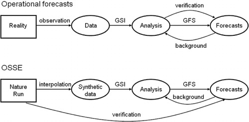
An OSSE consists of several components: a representation of the atmosphere called the Nature Run that plays the role of truth, usually a long, free numerical model forecast; synthetic observations that are extracted from the Nature Run fields for all existing and proposed observing systems; and a numerical weather prediction model and data assimilation system used for experimental forecasts. A diagram of the OSSE process is illustrated in Fig. 1. The European Centre for Medium-Range Weather Forecasts (ECMWF) created the Nature Run for the Joint OSSE using their operational forecast model in a 13-month integration. Synthetic observations have been developed both at the National Centre for Environmental Prediction (NCEP) and at the National Aeronautics and Space Administration (NASA) Global Modelling and Assimilation Office (GMAO). The forecast model used for the ESRL OSSE is the Global Forecast System (GFS) with the Gridpoint Statistical Interpolation (GSI) data assimilation package (DAS; Kleist et al., 2009).

Fig. 1.  Schematic diagram of ESRL OSSE components (bottom) versus real operational forecasting procedure (top).

The synthetic observations are ingested by the GSI data assimilation system, and observation impact may be calculated by comparing forecasts that include or exclude particular types of observations. The OSSE may also be used to investigate how data assimilation systems use different types of observations; because the ‘truth’ is fully known for the OSSE, evaluation of observation impact may be calculated in ways not possible with real observations.

Early attempts at OSSEs suffered from identical and fraternal twin problems, in which the same or very similar model(s) were used for both the Nature Run and forecast experiments (Arnold and Dey, 1986). These identical twin-model experiments suffer from insufficient model error that may bias conclusions about data impact, as described by Atlas et al. (1985). OSSEs have become more sophisticated over the past two decades as computing resources and model complexity have increased. OSSEs conducted at NASA's Goddard Laboratory for Atmospheres (Atlas, 1997; Atlas et al., 2001) were used to develop the methodology that led to the first beneficial impacts of satellite surface winds, as well as to evaluate the relative impact of temperature, wind and moisture data, the potential impact of a variety of space-based instruments and trade-offs in instrument design.

More recently, a Joint OSSE collaboration using a 1-month Nature Run from ECMWF yielded a number of OSSE studies for Doppler wind lidar (Marseille et al., 2001; Stoffelen et al., 2006; Masutani et al., 2010). OSSEs have also been conducted using a 3-month NASA generated Nature Run to evaluate the impact of wind lidar data on hurricane prediction (Atlas and Emmitt, 2008). By using an OSSE with an ensemble Kalman filter data assimilation system, Otkin et al. (2011) demonstrated the potential of an array of ground-based remote sensing boundary-layer profiling instruments to improve the accuracy of wintertime atmospheric analyses over land. Yussouf and Stensrud (2010) applied a similar approach to study the impact of phased array radar observations on very short-range prediction of severe thunderstorms. The current OSSE is a significant improvement in both the length and quality of the Nature Run, with more sophisticated synthetic observations than in previous global OSSEs.

It is necessary to calibrate the OSSE to ensure that the behaviour of the system is sufficiently similar to the real world for the results of the OSSE to be meaningful. In previous OSSEs, calibration metrics have included comparison of statistics of observation minus analysis and observation minus background for the OSSE vs. real data (Stoffelen et al., 2006) and comparison of observation impact through data denial experiments (Masutani et al., 2006; Atlas and Riishojgaard, 2008). In most OSSE studies, the calibration process was not used iteratively to improve the performance of the OSSE system, but in the current OSSE, the calibration process was used to adjust the OSSE system to attain more realistic results.

This paper describes the OSSE framework developed at ESRL and discusses the performance of the OSSE system along with the results of data denial experiments used to calibrate the OSSE system. Section 2 describes the components and overall set up of the OSSE, along with the calibration procedure. Evaluation of the performance of the OSSE system is discussed in Section 3. Discussion of the OSSE implementation process and uses of the OSSE system for exploration of the behaviour of data assimilation systems is given in Section 4. Results of experiments testing new observing systems will be addressed in future manuscripts.

2. OSSE setup

The process of performing an OSSE consists of several components: generation and evaluation of a Nature Run; generation and calibration of synthetic observations from the Nature Run; and experiments with new observation types and/or assimilation methods using a second forecast model. These experiments are then verified against the Nature Run.

2.1. Nature run

A Nature Run is a long, free forecast from a numerical weather prediction model; this plays the role of ‘truth’ for the OSSE. The Nature Run must be evaluated to determine whether the behaviour of the model is sufficiently similar to the behaviour of the real atmosphere, particularly in terms of spatial and temporal variability. Unlike the real atmosphere, the entire state of the Nature Run is known and is used to verify the results of the OSSE experiments. The Nature Run fields are also used as a basis from which synthetic observations are drawn.

The Nature Run was generated by ECMWF using their operational forecast model version c31r1, in a free run from 1 May 2005 to 31 May 2006 at T511 [approximately 45 km using an equal-area estimation (Laprise, 1992)] resolution with 91 vertical sigma levels and output at 3-hour intervals. This model version is similar to that used to generate the ERA-Interim re-analysis (Dee et al., 2011). Boundary conditions for sea surface temperature and sea ice were taken from the 2005–2006 archived dataset. The model output is available both on a reduced Gaussian grid at N256 with 1024 points at the equator on all sigma levels, and as a ‘quick-look’ 1° by 1° low-resolution dataset on 31 pressure levels for convenient data evaluation. The general circulation, tropical and mid-latitude waves, and tropical cyclones in the Nature Run have been investigated (Reale et al., 2007; McCarty et al., 2012), and the behaviour of the Nature Run has been found to be sufficiently realistic overall.

2.2. Forecast model

The forecast model used for experiments should be different from the model used to generate the Nature Run. If the same model or similar model versions are used for both the Nature Run and the forecast experiments, the forecasts will have insufficient model error growth and will evolve too closely to the Nature Run. Even when a completely different model is used for the forecast experiments, it is possible that the forecast model may behave more similarly to the Nature Run model than to the real atmosphere.

The numerical weather prediction model chosen for the experimental forecasts is the GFS with the GSI DAS. Both the model and DAS are from the February 2007 operational version from NCEP. The resolution of the GFS used here is T382 (approximately 60 km) with 64 vertical levels for experimental forecasts and T126 with 64 vertical levels for calibration experiments.

2.3. Synthetic observations

Simulated observations are extracted from the Nature Run fields for all data types that are currently ingested into the operational forecast model as well as for the proposed new data types. Ideally, the synthetic observations would be generated by careful simulation of all aspects of the observing system – i.e. by ‘flying’ satellites through the Nature Run with full inclusion of cloud effects and satellite orbits, and by calculating the advection of rawinsondes. In practice, some compromises are necessary when generating simulated observations. To create realistic synthetic observations, instrument and representativeness errors must be added to the observations. It should be noted that some degree of representativeness error is inherent in observations simulated from a high-resolution Nature Run and subsequently assimilated in a lower resolution forecasting experiment.

The basic method of generating synthetic observations for existing observational data types consists of interpolating Nature Run fields at times and locations of archived real observational data from the corresponding time period. For example, the synthetic observations for 25 July 00Z are based on the archived operational dataset from 25 July 00Z 2005. This retains a realistic distribution of observations in time and space with relatively little computational expense, but also introduces some potential discrepancies into the synthetic dataset. For example, the cloud distribution in the real world differs from that in the Nature Run, so observations such as cloud-derived wind vectors will be mismatched to the cloud distribution in the Nature Run. Similarly, real world rawinsonde profiles will have significant levels that are not representative of the Nature Run vertical structure. Aircraft tracks that reflect current weather patterns represent another discrepancy when applied on the Nature Run atmosphere.

Two synthetic observation datasets were developed from the Nature Run, one at GMAO/NASA, the second at NCEP/NOAA. The ESRL OSSE set up utilises the NCEP conventional dataset and both of the available radiance datasets. The two datasets are similar, both relying on an interpolation of relevant variables from Nature Run grids to observation locations. The main difference in the two conventional dataset occurs at or near the earth surface where NCEP extrapolates values to the observation topography, whereas GMAO uses the Nature Run topography to redefine the observation vertical locations.

Interpolation of the Nature Run fields was performed with first a bilinear horizontal interpolation, followed by a linear temporal interpolation, and then a log-linear interpolation in vertical pressure. One caveat of linear temporal interpolation is that non-stationary features, such as tropical cyclones, baroclinic lows and fronts, tend to be ‘smeared’ by the interpolation, with less accurate interpolation for faster-moving structures. Because of this, care should be taken when performing an OSSE to first evaluate whether specific phenomena of interest are adequately temporally sampled to be represented accurately in the OSSE.

The radiance observations for AMSU-A, AMSU-B, AIRS, HIRS-2, HIRS-3 and MSU generated by GMAO are described in Errico et al. (2013). The brightness temperatures were calculated from the Nature Run fields along vertical profiles using the Community Radiative Transfer Model (CRTM) version 1.2. Ideally, a completely different radiance scheme would be used for the forecast model compared to the generation of the synthetic observations, but the GSI employed the CRTM version 1.1. The dissimilarity in the CRTM versions results in synthetic radiance observations that are not perfectly interpreted when ingested into the GSI. The archived radiance dataset is thinned prior to generation of synthetic observations to reduce computational expense, although less thinning is applied than occurs within the GSI assimilation process. A simple treatment of clouds is used for calculations of infrared observations, using the cloud cover fraction of low-, high- and mid-level clouds from the Nature Run. Due to difficulties in generating microwave observations that are affected by surface emissivity over land or sea ice, observations for AMSU-A channels 1–6 and 15, AMSU-B channels 1–2, and MSU were assigned missing values over land or sea ice.

The simulation of radiance data at NCEP is very much the same as at GMAO except a different approach is taken in thinning the simulated datasets. Instead of attempting to explicitly account for cloudiness and cloud-affected radiances, the NCEP dataset used the operational thinning as recorded in diagnostic files from the GDAS assimilation cycle to locate footprints and channels to be simulated for the OSSE experiments. It could be pointed out this method contains the same discrepancy as was described regarding characteristics of rawinsondes, cloud winds and aircraft data that are not consistent with the Nature Run background. On the other hand, having an identical observation template helps to account for incidents such as data outages of particular observation types that can affect observation impact calculations.

In addition to radiance-based satellite datasets simulated in the NCEP project, the SBUV ozone retrievals of layer ozone amounts were simulated. A simple conversion is made from Nature Run ozone mixing ratio profiles to OSBUV retrieval layer ozone quantities to simulate this data source. OSBUV data are assimilated as retrieved profiles. GOES radiance observations were also generated for the NCEP radiance dataset, but are not included in the GMAO dataset.

Observation errors were added to the perfect synthetic data to introduce both instrument and representativeness errors using an early version of the methods described in detail by Errico et al. (2013). Random errors were generated from a normal distribution with mean of zero and SD specified per observation type. The errors for conventional data types were uncorrelated with the exception of sounding observations, for which vertically correlated errors were generated. Most radiance observation errors are horizontally correlated, with the exception of GOES radiance and OSBUV (ozone) observations. The errors differ from those described in Errico et al. (2013) as follows: satellite wind errors including both feature-tracking winds and scatterometer winds are uncorrelated; satellite radiance errors are generated using the GSI error tables and are not refined for individual channels; satellite radiance correlation lengths are not calibrated. The impact of using uncorrelated rather than correlated errors for radiance observations is discussed in detail by Errico et al. (2013).

2.4. Calibration

As the Nature Run is not a perfect representation of the real atmosphere, and the synthetic observations are likewise not perfect representations of real observations, it is not expected that the data impact of the synthetic observations in the OSSE system will be identical to the data impact of real observations. In the calibration process, the added synthetic observation errors are adjusted so that the statistical behaviour of the synthetic observations in the forecast model and data assimilation system is as similar as possible to the statistical behaviour of real observations.

A different approach to calibration is taken in comparison to previous OSSEs. Instead of only using the calibration to inform the interpretation of the OSSE results (as described by Atlas, 1997), an iterative process was used to modify the observation error in order to ‘tune’ the data impact on the analysis field in the OSSE system. The analysis impact of the conventional synthetic observations is adjusted by altering the random errors, which are applied to the perfect synthetic data. The SDs of random errors with Gaussian distribution are changed as a function of pressure for conventional observations. The starting values of the error SDs for the iterative process are the observational error variances used by GSI during assimilation.

Ideally, the observation impact on the forecast skill would be used to tune the system, as it is this impact that is often of primary interest when performing an OSSE. There are several impediments to this approach, however. Forecast skill and predictability is highly variable in time, so that a lengthy period of forecasts would be required to conduct a definitive comparison between the OSSE and real data. Model error plays a large role in medium-range forecast skill, and discrepancies in the relative model error between the forecast model and the Nature Run compared to the model error between the forecast model and the real world can be very important. One way to help evaluate the OSSE performance regarding forecast skill and observation impact would be to run a series of ensemble forecasts with data denial experiments for both real data and the OSSE over several months. The ensemble spread of forecast skill compared between the OSSE and real data would help to indicate differences in model error. These forecast skill calibrations would be extremely computationally expensive and are beyond the currently available resources.

Another difficulty with using the forecast skill for tuning the OSSE is that modifying the observation error characteristics may not be an effective method of altering the observation impact on medium-range forecasts. The growth of model error may be unrealistic in an OSSE, in both large scale error growth and in error growth of specific processes. Depending on the particular discrepancies in model error in the OSSE compared with real data, some types of observations may demonstrate incorrect observation impacts as a result. Attempting to tune the observation errors in order to adjust the forecast impact when the model error growth is actually at fault, may result in overcompensation or insensitivity of the observation impacts to observation errors. It is not clear that a tuning method is possible wherein all possible metrics of interest can be simultaneously tuned in an acceptable fashion. The solution chosen here is to select a metric that can be tuned with moderate use of resources. After completion of the tuning process, the OSSE performance is then evaluated for a longer period for metrics of forecast skill and observation impact. It is hoped that the chosen tuning metric will also result in acceptable OSSE behaviour for these additional metrics.

While the synthetic errors are altered during calibration, the background and observation error variances used by GSI are not changed. As a result, the relative weighting of the observations and background fields (i.e. the gain K) is unchanged during the calibration process and matches the weighting used by the operational GSI. Using standard notation, the analysis state x _a is calculated as1

where x _b is the background state, y _o are the observations, and H is the operator that transforms the background state into observation space. Since y _o can be considered the sum of the ‘perfect’ observation and the observation error, the gain acts on both the perfect observation and the observation error. Using a 6-hour forecast from the previous cycle as the background state, it has been found (Errico et al., 2013) that x _b is relatively insensitive to changes in y _o, and thus x _a can be manipulated by changing the observation error.

A rapid calibration method was used to perform preliminary calibration and tuning of all conventional data types. Archived real data from the same period as the Nature Run were used for verification – these data have the same temporal and spatial distribution as the synthetic observations. The analysis impact is considered here as the global root-mean-square difference between the control analysis and the data denial analysis:2

where I _a is the analysis impact, A _d is the data denial analysis field, A _c is the control case analysis field, φ is latitude and λ is longitude. In these cases, 2-week data denial experiments were performed for groups of similar observation types for the period 1 July to 15 July 2005 using a lower resolution of the GFS at T126 (approximately 180km resolution). This reduced resolution was chosen to expedite the calibration process due to the large number of extended model experiments needed for calibration while retaining adequate representation of long-wave behaviour in the forecasts. The analysis impact rapidly increases during the first few days as the system adjusts to the sudden removal of an observation type, and then asymptotes to a steady value after the first week. Examination of the analysis impact over longer 6-week calibration runs shows that the impact remains at this steady value over the entire period, except for short periods in the event of data outages. The steadiness of the analysis impact metric indicates that the short 2-week period is sufficient for the purposes of tuning the OSSE.

To tune the observation error variances, the OSSE analysis impact was compared to the real data analysis impact for the same time frame, and the synthetic error variances were adjusted to nudge the analysis impact of the synthetic data types toward the real data analysis impact. In general, (de)increasing the error SD resulted in an (de)increase in analysis impact as will be discussed in the next paragraph, although in some instances the analysis impact was insensitive to the observation error. A new set of synthetic observations with the adjusted errors was generated and used for a new data denial case. This cycle of error adjustment and data denial experiments was repeated until the analysis impact of the synthetic observations matched the real data analysis impact as closely as possible. In some cases, the synthetic data analysis impact could not be adjusted to match the real data analysis impact at all (or any) vertical levels; this was most common at levels near the surface where differences in the real and Nature Run topographies are important, and near the tropopause where conventional observations are often sparse.

The analysis impact is expected to increase when the SD of the applied observation errors increases because the ingestion of larger errors results in a control analysis field that has larger deviations from the data denial analysis field. Only when the observation error is large enough to cause removal of the observation due to quality control will the analysis impact decrease with increasing observation error as more observations are removed by quality control in the DAS. Thus, analysis impact is a measure that does not discriminate between improvements and degradations of the analysis field due to ingestion of an observation type.

Observational errors for radiance data were not adjusted in the same manner as the conventional observations, the error covariances used for the radiance data match those employed by the GSI. The error SD for radiance observations was assigned per satellite channel, and initial tests of adjustments to the error statistics showed that the analysis impact of satellite data was much less sensitive to the magnitude of uncorrelated observational errors than the conventional observations. This insensitivity was due to the use of uncorrelated errors in the initial calibration tests, greater sensitivity is expected for correlated errors that were added to the final radiance observation dataset. The impacts of correlated errors are discussed in detail by Errico et al. (2013). The only exceptions to this were OSBUV and GOES radiance observations, which were excluded from the GMAO dataset; for these observation types, uncorrelated errors with SDs taken from the GSI operational tables were used. Due to time constraints, iterative calibration of the applied errors of radiance observation was not attempted.

2.5. Calibration effects

Adjusting the observation error during the calibration process affects the quality of the background and analysis fields as well as the quality of the observations. Observation minus forecast (O−F) statistics give an indication of the disparity between the observations and the model fields in a metric that combines the growth of error during forward integration of the model with the observation errors. Figure 2 illustrates the statistics of observation minus analysis (O−A, green symbols), observation minus background (O−B, red symbols), as well as observation minus the 24-hour forecast (O−F ₂₄, dark blue symbols) and observation minus 48-hour forecast (O−F ₄₈, cyan symbols) before and after the calibration procedure for rawinsondes; Fig. 3 shows similar results for aircraft data types. Each panel in Figs. 2 and 3 compares the RMS for real data (abscissa) with the RMS for the OSSE (ordinate); each symbol plotted represents the global root-mean-square difference between the observations and forecast field for one cycle time at a particular vertical level. Ideally, the data points would be scattered symmetrically about the line x=y in the calibrated system.

Fig. 2.  Comparison of real data and OSSE O−F statistics for rawinsonde observations, each symbol indicates the global RMS O−F for a certain vertical level for 1d of the calibration period. Green symbols indicate O−A, red symbols indicate O−B, dark blue symbols indicate O−F for the 24hour forecast and cyan symbols indicate O−F for the 48hour forecast. Plus signs indicate the 1000hPa level, open circles the 850hPa level, closed circles the 500hPa level, open squares the 300hPa level, closed squares the 250hPa level, multiplication signs the 200hPa level, open diamonds the 150hPa level, open triangles the 100hPa level and closed triangles the 50 hPa level. (a, b) T126 OSSE prior to calibration, 5 July to 31 July 2005; (c, d) T126 OSSE after calibration, 5 July to 31 July 2005; (e, f) T382 OSSE after calibration, 5 August to 31 August 2005.

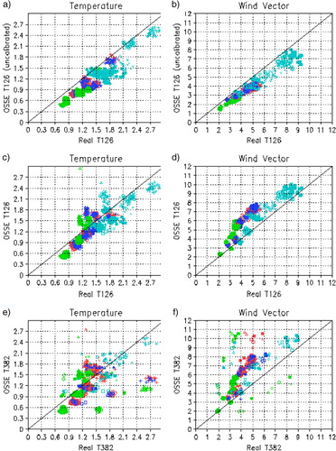
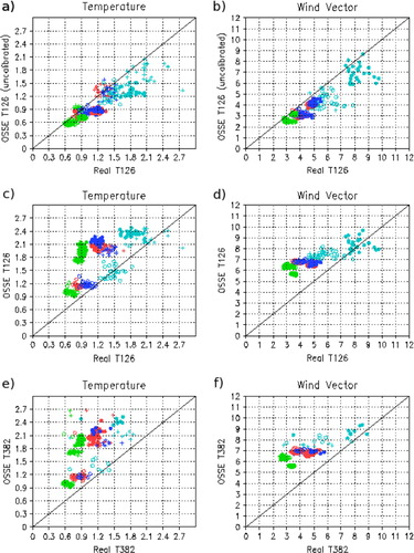
Fig. 3.  Comparison of real data and OSSE O−F statistics for aircraft observations, each symbol indicates the global RMS O−F for a certain vertical level for 1d of the calibration period. Green symbols indicate O−A, red symbols indicate O−B, dark blue symbols indicate O−F for the 24hour forecast and cyan symbols indicate O−F for the 48hour forecast. Plus signs indicate the 1000–700hPa range, open circles the 700–300hPa range and closed circles the 300–150hPa level range. (a, b) T126 OSSE prior to calibration, 5 July to 31 July 2005; (c, d) T126 OSSE after calibration, 5 July to 31 July 2005; (e, f) T382 OSSE after calibration, 5 August to 31 August 2005.

Prior to calibration, it is noted that the RMS for O−F are generally lower in the OSSE compared to the real data statistics, indicating that either or both the observation error or the forecast error is too small. By increasing the observation error variance during the calibration process, both the observation and forecast errors are increased, but the forecast error tends to increase at a slower rate than the observation error, as some of the observation error is diminished during the assimilation process and forward model integration. As a result, the RMS O−F for the OSSE tend to increase when the observation errors are increased.

The changes in the RMS O−F due to calibration of the observation errors show mixed results. For some observations, such as RAOB humidity data, the RMS O−F is improved by calibration, with the calibrated OSSE RMS O−F showing similar distribution to that of real RMS O−F in the middle and upper troposphere. The lower troposphere and near-surface RMS O−F were not strongly affected by the calibration process, as was also noted during calibration of the analysis impact. In some cases, the calibrated O−F RMS is larger than for real data, such as for RAOB wind observations in the middle and lower troposphere and for aircraft temperature and wind data. When the calibrated O−A RMS is much higher than for real data, this indicates that the observation error is overinflated in order to compensate for other deficiencies in the OSSE. These deficiencies could include insufficient model error and incorrect spatial or temporal correlations of observation error.

The RMS O−A has the lowest values, with RMS of O−B and O−F ₂₄ being of similar magnitude for both real data and the OSSE. The RMS O−F ₄₈ has the largest values, as expected. For the data that has RMS O−A distribution close to that of real data, the growth in RMS O−F with forecast time occurs at a similar rate in the OSSE compared to real observations. However, in cases where the calibrated OSSE data have RMS O−A that is significantly larger than for real data, the change in RMS O−F with forecast time is slower in the OSSE than for real data. This is most clearly illustrated for aircraft observations, where the RMS O−A is too high in the calibrated OSSE, but the RMS O−F ₄₈ is much closer to the real data distribution. The uncalibrated OSSE aircraft data have a faster growth of RMS O−F with forecast time. Only a fraction of the analysis error field experiences growth during forward integration while other analysis errors are damped; if the additional analysis errors present in the calibrated case grew at the same rate as the errors in the uncalibrated case, the O−F ₄₈ should also be higher in the OSSE than the real data. The net analysis error that grows during the first 48hours of the forecast does not appear to be strongly impacted by increased observation errors added during the calibration process, possibly because the explicitly added observation errors for aircraft data are spatially uncorrelated, and the forward model integration tends to filter and damp out uncorrelated errors more readily than correlated errors.

The lower panels of Figs. 2 and 3 show the RMS O−F statistics for the T382 cases for comparison with the T126 calibration experiments. The T382 results show more scatter of the RMS O−F, but otherwise, the distribution of RMS O−F is very similar to the T126 cases. This result implies that the calibration can be performed at lower resolution and the results transferred to higher resolution.

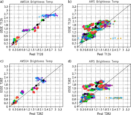
Although the radiance observation errors were not iteratively calibrated, the statistics of O−F are shown for AMSU-A and AIRS observations in the OSSE in comparison to real data at both T126 and T382 resolution in Fig. 4. For AMSU-A, the RMS O−A, O−B and O−F distributions are generally in agreement between the real and OSSE cases, with values close to the x=y line. Increasing the resolution from T126 to T382 maintains this agreement, but the RMS O−F values decrease for channels 11 and 14. AIRS data show less agreement of O−F statistics between the real and OSSE cases, with some channels having much higher or lower RMS O−F in the OSSE. Particularly notable are a few AIRS channels where the RMS O−F appears to be nearly fixed at a low value in the OSSE with much higher RMS O−F for the real data. Although there are some badly mismatched channels for AIRS, the bulk of the channels have RMS O−F that is symmetric about x=y.

Fig. 4.  Comparison of real data and OSSE O−A and O−B statistics for AMSU-A and AIRS brightness temperatures, each symbol indicates the global RMS O−A or O−B for a particular channel at 0000 UTC for 1d of the calibration period. For AMSU-A, the channel colours are 1: black; 2: red; 3: green; 4: dark blue; 5: light blue; 6: magenta; 7: yellow; 8: orange; 9: purple; 10: yellow–green; 11: medium blue; 12: dark yellow; 13: aqua; 14: dark purple; 15: grey. For AIRS, these colours are rotated though the channel sequence, with every other channel plotted. O−A and O−B are plotted with the same symbol and colour for each channel, the O−A cluster has smaller RMS than the corresponding O−B cluster. (a, b) T126 OSSE, 5 July to 31 July 2005; (c, d) T382 OSSE, 5 August to 31 August 2005.

2.6. Calibration verification

Following the ‘quick calibration’, extended data denial cases were performed over a 6-week period to verify that the tuning process was successful. These data denial cases were performed both for the synthetic observations and for archived real observations from the same time period so that the OSSE behaviour could be compared with real data impacts. Five data denial cases were selected for these longer tests: RAOB, aircraft, AMSU-A, AIRS and GOES radiance, which were compared to a Control case in which all data types were included. The GFS/GSI was then cycled at T126 from 1 July 2005 to 21 August 2005, and the differences between the Control results (including all data types) and the data denial cases were examined. The evaluation of rawinsonde (RAOB) data impact was repeated at T382 resolution after calibration of the entire conventional dataset for both real and synthetic data. The RAOB impact was similar for the synthetic and real data at T382, indicating that the calibration at T126 may be used for higher resolution runs.

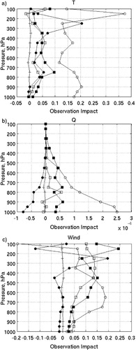
The analysis impact I _a defined in eq. (2) is calculated for the five observation data types tested in data denial experiments; the results for global averages for the 15 July–20 August period are shown in Fig. 5. For horizontal winds, the u and v wind vector components are used in a combined metric in eq. (2). In general, the analysis impact is similar for the real and OSSE systems, with the relative ranking of impact from different observation types being the same for most fields and levels. One major exception is AMSU-A, which has too little impact in the lower troposphere in the OSSE, with RAOB types reflecting greater impact at these levels. This is most likely due to the treatment of AMSU-A, where near-surface channels over sea ice and land are omitted from the synthetic observations. The peak in aircraft analysis impact for wind and temperature at the 200–300hPa level is well-represented in the OSSE system. GOES radiance has the smallest analysis impact in both the real data and OSSE systems, but the amplitude of the impact is somewhat too weak in the OSSE. This may be due to the use of errors for GOES radiances that are spatially uncorrelated; because the analysis impact does not discriminate between beneficial and detrimental impacts, the greater degradation of the analysis field caused by the ingestion of correlated observation errors would result in an increase in the analysis impact.

Fig. 5.  Global observation impact on the analysis field as a function of pressure level from data denial cases, from 15 July to 15 August 2005. Left, real data cases; right, OSSE cases with GMAO radiance observations. Top, temperature T (K); centre, specific humidity q (kg/kg); bottom, horizontal wind (m/s). RAOB impact, open circles; Aircraft impact, filled circles; AMSU-A impact, open squares; AIRS impact, filled squares; GOES radiance impact, crosses.

The spatial distribution of analysis impact is shown in Figs. 6 and 7 for select fields at 500hPa. The distribution of analysis impact for the OSSE system shows gross agreement with the distribution for real observations. The relative impact over land vs. ocean, tropics vs. mid-latitudes vs. Polar Regions, and Northern vs. Southern Hemisphere are adequately represented overall. The AMSU-A analysis impact in the OSSE has areas of reduced impact over continents due to the omission of the channels that are affected by the surface; this is not observed for real data.

Fig. 6.  Analysis impact maps, 500hPa geopotential height, for real data denial cases from 15 July to 15 August 2005. Contour interval 2.5m.

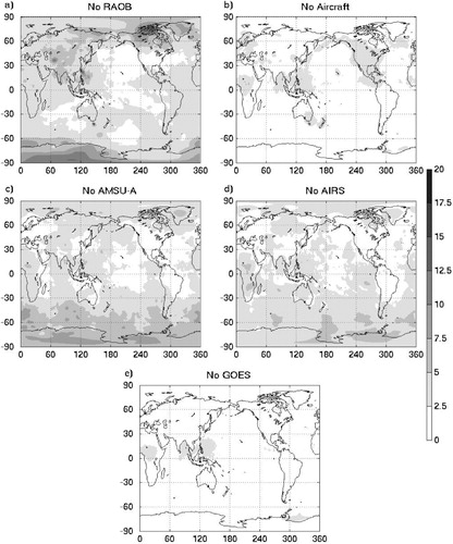
Fig. 7.  As in Fig. 6, but for OSSE data denial cases from 15 July to 15 August 2005.

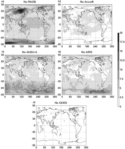
There are some regions which show significant bias in the OSSE system compared to real observations: RAOBs in particular have a very large impact over Siberia in the OSSE which is not seen for real observations, as well as slightly greater impact across the tropics. The synoptic pattern in the Nature Run during July–August (not shown) features a strong ridge over eastern Europe and a persistent trough over Siberia; this unusual pattern may contribute to the anomalously large RAOB impact over eastern Asia. This impact may be particularly large due to the lack of lower tropospheric AMSU-A channels that might compensate in the RAOB denial case. It is unlikely that differences in the observation errors of the OSSE compared to real observation errors would cause such a localised, persistent anomaly; if large RAOB errors were the cause, similar anomalies would be expected over regions such as South America and Australia. This type of persistent anomaly may affect the tuning process if the magnitude and spatial area of the anomaly is sufficiently large to impact the global values of analysis impact. One possibility for mitigating this type of problem is to restrict the region over which the analysis impact is calculated to exclude the area of anomalous behaviour.

While the comparison of analyses and forecasts is the only way to evaluate data impact in the real world, as the actual state of the atmosphere is unknown, for the OSSE system comparisons can be made using the ‘truth’, i.e. the Nature Run. The observation impact is calculated as3

where I _o is the observation impact, A _d is the data denial analysis field, A _c is the control analysis field, A _N is the Nature Run field, φ is latitude and λ is longitude. This gives a measure of relative data impact for each observation type. It is possible for a data type which gives a large impact with respect to the analysis to give a small or negative observation impact in relation to the Nature Run. This occurs when the inclusion of the data type significantly adjusts the analysis field during data assimilation, but not in such a way as to bring the analysis closer to the truth. These differences could be caused by large error variances of the observations or by poor handling of the observations by the data assimilation system.

Figure 8 shows the observation impact of five observation types in relation to the Nature Run. It is notable that the relative importance of the data types is not always consistent with the analysis impact of the data types shown in Fig. 5. For example, GOES radiance has a small but non-negligible impact compared to the control analysis, but a near-zero impact when compared with the Nature Run for all areas, fields and levels. In the Northern Hemisphere mid-latitudes, the observation impact for radiance types is much smaller in comparison to the observation impact for RAOB, in contrast to the analysis impact where AIRS and AMSU-A show a moderate impact. While aircraft data show a significant impact on wind and temperature at flight levels both for the observation impact and analysis impact, the aircraft observation impact from the surface to 400hPa shows negative (detrimental) impact for the wind field.

Fig. 8.  Global observation impact for OSSE data denial cases from 15 July to 15 August 2005, calculated using the Nature Run for verification. Top, temperature T (K); centre, specific humidity q (kg/kg); bottom, horizontal wind (m/s). RAOB impact, open circles; aircraft impact, filled circles; AMSU-A impact, open squares; AIRS impact, filled squares; GOES radiance impact, crosses.

3. Forecast skill validation

In addition to the data denial impacts on the analysis previously described, 5-d forecasts were generated for each data denial case over the 6-week validation period, with forecasts launched each day at 0000 UTC and 1200 UTC. Two aspects of the forecast skill are investigated: the relative skill of the OSSE control forecasts compared to real data forecasts, and the impact of observations on forecast skill determined through data denial experiments. Ideally, the OSSE forecasts would show similar mean and distribution of skill as real data forecasts, and likewise similar observation impacts on forecast skill. As analysis impact rather than forecast impact was the metric used for tuning the synthetic observation error, there is no guarantee that the OSSE forecast behaviour will mimic that of real data forecasts.

3.1. Anomaly correlation

The skill of the 5-d forecasts is measured using the metric of anomaly correlation. Forecast skill is explored both at the lower T126 resolution used in the calibration experiments and at the higher T382 resolution that would be used for future OSSE cases.

3.1.1. T126 resolution.

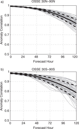
Anomaly correlation is calculated for 500hPa geopotential height using the NCEP reanalysis long-term July mean field as the climatology. Figure 9 shows the anomaly correlation for individual forecasts and forecast mean taken from 15 July to 15 August for the real data and OSSE forecasts. The mean and SD of the anomaly correlation coefficients at the 120-hour forecast are shown in Table 1 for the control cases using real data, the GMAO synthetic observation dataset and the NCEP synthetic observation dataset. There is no statistically significant difference (using a Mann–Whitney U test at 95% confidence) between the 120-hour anomaly correlation of the GMAO dataset run compared to the NCEP dataset run. The GMAO dataset run has lower median skill from the real data case in the Northern Hemisphere and higher median skill in the Southern Hemisphere at 95% confidence, while the NCEP dataset case shows significantly lower skill in the Northern Hemisphere but marginally significant difference (94.7% confidence) for the Southern Hemisphere.

Fig. 9.  Anomaly correlation for 500hPa geopotential height, calculated using analysis fields for verification, from 15 July to 15 August 2005. Individual forecasts: grey lines; mean of all forecasts: solid black line; one SD from mean: dashed black lines. (a, b) Real data control case; (c, d) OSSE control case with GMAO radiance; (e, f) OSSE control case with NCEP radiance. (a, c, e) 30°N–90°N; (b, d, f) 30°S–90°S.

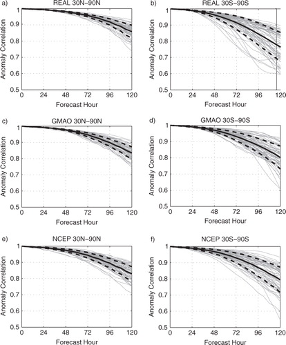
Table 1. Mean, µ, and standard deviation, σ, of 120-hour forecast anomaly correlation for 500 hPa geopotential height, 15 July to 15 August 2005

Experiment	NH µ	NH σ	SH µ	SH σ
Real T126 control	0.858	0.040	0.764	0.090
GMAO T126 control	0.835	0.037	0.801	0.071
NCEP T126 control	0.830	0.044	0.794	0.078
GMAO T126 vs. NR	0.816	0.041	0.786	0.070
GMAO perfect obs	0.847	0.043	0.823	0.063
Real T382 control	0.848	0.042	0.786	0.086
GMAO T382 control	0.854	0.039	0.829	0.055
NCEP T382 control	0.814	0.060	0.814	0.050

Northern Hemisphere (NH) areal mean from 30°N–90°N; Southern Hemisphere (SH) areal mean from 30°S–90°S.

The real data control case has relatively high 120-hour forecast skill for the last 2 weeks of July (not shown), but there are multiple periods of low forecast skill during August in the Southern Hemisphere. For the OSSE, there are brief periods of low forecast skill in the Southern Hemisphere in both the third week of July and early August in both the GMAO and NCEP dataset cases. The Northern Hemisphere does not show any incidents of very low skill for either the real control or OSSE cases.

With only 1month of forecasts available, it is difficult to determine the cause of differences in skill between the OSSE and real data cases. The individual months may also differ in the predictability of the overall synoptic pattern in the Nature Run vs. the real case. The discrepancy in relative skill between the Northern and Southern Hemispheres could be due to seasonal effects, with strong baroclinicity in the winter Southern Hemisphere compared to a more convective regime in the Northern Hemisphere summer. While a lengthier validation period would be ideal, resource availability limits the time span to a single month. The variability of skill is similar between the OSSE and real observations in the Northern Hemisphere, but the variability is smaller in the OSSE system in the Southern Hemisphere compared to real data. It is unclear if the difference in Southern Hemisphere variability is significant due to the relatively small sample size.

The anomaly correlation is most often calculated using the analysis sequence as verification; for the OSSE system, the anomaly correlation can be calculated using the Nature Run as actual truth. Anomaly correlations calculated in this fashion for the GMAO synthetic observation dataset analysis sequence are shown in Fig. 10 and listed in Table 1 as ‘GMAO T126 vs. NR’. The anomaly correlation calculated in this fashion is 0.019 lower in the Northern Hemisphere and 0.015 lower in the Southern Hemisphere than the analysis-verified anomaly correlation metric for the 5-d forecast.

Fig. 10.  Anomaly correlation for 500hPa geopotential height, calculated using Nature Run fields for verification, mean of forecasts from 15 July to 15 August 2005 as in Fig. 9. OSSE control case with GMAO radiance; (a) 30°N–90°N; (b) 30°S–90°S.

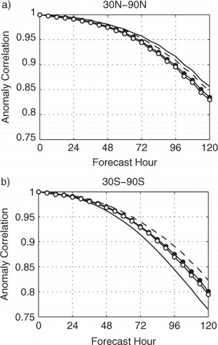
The OSSE framework enables investigation of the role of observation error, as ‘perfect’ synthetic observations are available for all data types. The cycling experiments are repeated using only synthetic observations with no added errors over the entire integration period for the GMAO synthetic dataset. The resulting anomaly correlations for the forecasts are shown in comparison to the error-added observation forecasts in Fig. 11 and in Table 1 as ‘GMAO Perfect Obs’. The decrease in the anomaly correlation coefficient of the 120-hour forecast when errors are added in comparison to the perfect observations is 0.12 in the Northern Hemisphere and 0.22 in the Southern Hemisphere.

Fig. 11.  Mean anomaly correlation for 500hPa geopotential height for forecasts from 15 July to 15 August 2005. Solid black line, real data control; dashed line, ‘perfect’ OSSE control with GMAO radiance; dotted line with filled circles, error-added OSSE control with GMAO radiance; dotted line with open circles, error-added OSSE control with NCEP radiance observations. (a) 30°N–90°N, (b) 30°S–90°S.

3.1.2. T382 resolution.

The OSSE experimental forecasts are performed at T382 resolution, so it is of interest to determine if there are significant differences between the OSSE behaviour at the full resolution and at the lower T126 calibration resolution. Due to the computational expense of the higher resolution forecasts, control runs at T382 are generated for the period 1–30 August 2005 for real data and for synthetic observations. Anomaly correlations are calculated for 120-hour forecasts from 5 August to 25 August 2005 and are shown in Fig. 12.

Fig. 12.  Mean anomaly correlation for 500hPa geopotential height for forecasts from 1 August to 31 August 2005, as in Fig. 9 but for T382 cases. (a, b), real data control case; (c, d) OSSE control with GMAO radiance; (e, f) OSSE control with NCEP radiance. (a, c, e), 30°N–90°N; (b, d, f) 30°S–90°S.

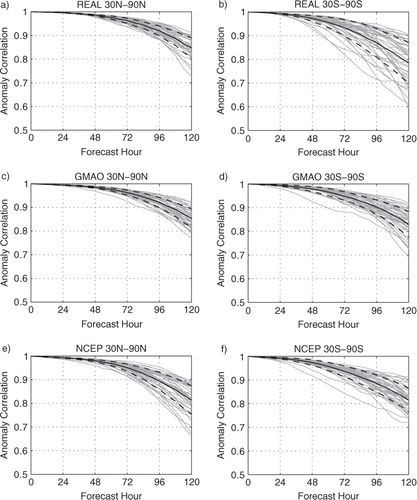
As in the T126 cases, the real data control at T382 showed multiple episodes of low skill forecasts in the Southern Hemisphere during the first half of August, with higher skill during the third week of August. Both OSSE cases featured high skill in the Southern Hemisphere during mid and late August, with a period of lower skill during early August. There were no incidents of low-skill ‘drop-outs’ in the OSSE cases in the Southern Hemisphere, although several ‘drop-outs’ were observed in the real data control. In the Northern Hemisphere, the real data control had relatively high skill during early and late August, with a period of lower skill during the second week of August. The GMAO dataset case showed consistently high skill throughout the month of August, but the NCEP dataset case showed two cases of low forecast skill later in August.

In the Southern Hemisphere for all datasets, mean anomaly correlation coefficients for the T382 120-hour forecasts increase by 0.02–0.03 in comparison to the T126 cases, as seen in Table 1. However in the Northern Hemisphere, the anomaly correlation only increases for the case with GMAO synthetic observations, the anomaly correlation decreases for both the real observations and NCEP synthetic observations. At T382, the GMAO dataset run skill is significantly higher than the real data skill in the Southern Hemisphere but there is not a significant difference in skill in the Northern Hemisphere, while the NCEP dataset run skill is significantly smaller than the real data skill in the Northern Hemisphere but there is no significant skill difference in the Southern Hemisphere. The skill of the GMAO dataset run is significantly different from the skill of the NCEP dataset run in both hemispheres at T126 and T382, with the NCEP dataset resulting in overall lower anomaly correlations. While the conventional observations are fairly similar in both datasets, there may be more significant differences in the radiance observations that result in the consistently higher anomaly correlations for the GMAO dataset compared with the NCEP dataset.

3.2. Data impact: forecasts

As the OSSE system is intended to evaluate the use of new observing data in improving forecasts, the impact of observational data on forecasts in the OSSE system is crucial. Anomaly correlations of the data denial experiments are used to quantify the data impact on forecasts. The anomaly correlation impact (ACI) is calculated as4

where ACC _di is the anomaly correlation coefficient of the ith data denial forecast, ACC _ci is the anomaly correlation coefficient of the ith control forecast, for K=62 forecasts from 15 July to 15 August 2005 at 0000 UTC and 1200 UTC. A positive ACI indicates that removal of an observation type reduces the anomaly correlation of the forecasts. ACI is calculated for the extratropics of each hemisphere and the results are shown in Fig. 13.

Fig. 13.  Anomaly correlation impact of data denial cases from 15 July to 15 August 2005. (a, c) Real data cases; (b, d) OSSE cases. (a, b) 30°N–90°N; (c, d) 30°S–90°S. RAOB impact, open circles; aircraft impact, filled circles; AMSU-A impact, open squares; AIRS impact, filled squares; GOES radiance impact, crosses.

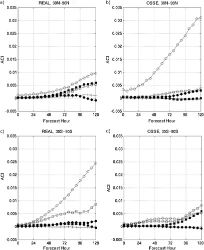
Agreement between the OSSE and real data ACI is best for AMSU-A and GOES radiance data types. There is a sign difference in the anomaly correlation impact for AIRS observations in the Northern Hemisphere, with negative impact in the extended forecast in the OSSE system, but a strong positive impact for real data. In the Southern Hemisphere, the AIRS ACI is much larger in the extended forecast for the OSSE system in comparison to real data. RAOB impact also shows significant discrepancies, with nearly three times greater ACI in the OSSE system at the 120-hour forecast in the Northern Hemisphere, but ACI five times smaller in the OSSE than with real data in the Southern Hemisphere. The large ACI for RAOB in the OSSE case may be related to the large RAOB analysis impacts observed over eastern Asia in Fig. 7. Anomaly correlation is influenced by both model error and initial condition error, with model error playing a large role at extended forecast periods. The discrepancies in ACI between the OSSE and real data cases may be due to differences in model error relative to the Nature Run vs. the real world. The nature of the observation error may also impact the ACI, as the synthetic errors lack intentionally added bias and may have errors that do not have realistic spatial correlations.

The root-mean-square error between the forecast fields and the analysis sequence (not shown) reveals similar overall magnitudes and spatial distribution in the OSSE and for real data. The fastest error growth is seen in the Southern (winter) Hemisphere mid-latitudes and Polar Regions, as well as the Arctic, although the errors are somewhat weaker in these areas in the OSSE compared to the real data case.

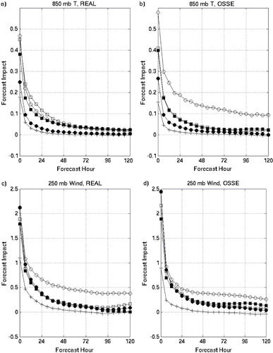
Forecast impact is calculated similarly to analysis impact:5

where F _d is the data denial forecast field and F _c is the control case forecast field. Unlike anomaly correlation, forecast impact is useful in tropical areas for certain fields. Figure 14 shows forecast impact for temperature at 850hPa and for horizontal winds at 250hPa. Comparison of Fig. 14a and b shows similar temperature forecast impact for most of the tested observation types, with the exception of RAOB data which has much too strong of an impact in the OSSE in relation to the real data case. This is somewhat explained by the large anomaly over Siberia that was seen in the OSSE analysis impact in Fig. 7a. There is better agreement for RAOB impact for 250hPa horizontal wind, shown in Fig. 14c and d. GOES radiance wind impact decreases more rapidly in the first 12hours of the forecast in the OSSE system than for real observations.

Fig. 14.  Global forecast impact for data denial cases from 15 July to 15 August 2005. (a, c) Real data cases; (b, d), OSSE cases. (a, c), 850hPa temperature impact, K; (b, d) 250hPa horizontal wind impact, m/s. RAOB impact, open circles; Aircraft impact, filled circles; AMSU-A impact, open squares; AIRS impact, filled squares; GOES radiance impact, crosses.

4. Discussion

The current Joint OSSE effort represents an advance in the sophistication of global OSSE studies. The Nature Run is considerably longer and at higher resolution, and the synthetic observations have been generated with more realism than previous OSSEs. While improvements to the OSSE setup are on-going, it is hoped that the Joint OSSE effort will provide a resource for the study of observing systems and data assimilation systems for years to come. The particular set up of the OSSE described herein was conscribed in part by limited computing resources and the desire for timely experimental results. The synthetic datasets and the method of calibration used are preliminary versions, and it is anticipated that significant modifications may be made in the future.

The explicitly added observation errors are one of the few elements of the OSSE that are easily adjusted, in comparison to the quality of the Nature Run, the forecast model skill, or the sophistication of the synthetic observation generators. While the analysis impact and innovation statistics of the synthetic observations may be calibrated to a certain extent by modifying the methods used to create the observations or the error characteristics of the observations, adjusting the impacts of the observations on the forecast field is much more difficult, particularly at longer forecast lead times. Changes to the observation errors have the greatest impact on the statistics of O−F, where the observation error directly influences the metric. The analysis and background fields and their statistics of A–B are only indirectly influenced by the observation errors, and the assimilation process and forward model integration between cycles tends to diminish the impact of observation errors on these metrics. As the model is integrated into the medium-range forecast period, the influence of observation errors decreases even further, so that there is only minor impact on metrics such as anomaly correlation and RMS forecast errors.

The statistics of O−B, O−A and O−F further indicate that the calibration of conventional observations in some cases tends to overcompensate for deficiencies in the OSSE setup, resulting in excessively inflated observation errors compared to real data. One possible cause of too-small observation impact is insufficient model error, where the forecast model behaviour is more similar to the Nature Run behaviour than to the real atmosphere. Another possible cause is observation errors that are not realistically correlated either temporally or spatially. Uncorrelated observation errors are more readily removed during the data assimilation process than correlated errors, as the GSI assumes that the observation errors are uncorrelated. Although some spatial correlation of observation errors has been included in the synthetic observations, no temporal correlation has been included.

When calibrating an OSSE, there are several different options to choose from when selecting the metrics used for tuning. In this work, the observation impact on the analysis field has been selected, as this metric is one that might be used to quantify the role of new observation types in future OSSE experiments. In contrast, the O−A or A−B metrics might have been used, although the results of the Errico et al. (2013) study imply that doing so would have resulted in analysis impacts that were smaller in the OSSE than for real observations. Likewise, the medium-range forecast impacts could have been used as the tuning metric, possibly resulting in even greater overinflation of observation errors during the calibration process if model error is insufficient in the OSSE. Forecast impact metrics are much more computationally expensive for tuning an OSSE than metrics of analysis impact, observation innovation, or analysis increments. It is not possible to simultaneously tune the OSSE for all metrics, so instead a single metric is selected for tuning and the other metrics are evaluated after tuning is complete. If some significant discrepancy is noted in these additional metrics after tuning, the option remains to retune the OSSE using an alternative metric or to look for more fundamental problems with the OSSE framework, such as insufficient model error.

The 5-d forecast skill of the OSSE was compared to the skill of the real system using the anomaly correlation of 500hPa geopotential height. Because the predictability of the atmosphere can vary significantly with time, the month-long period examined here is not sufficient to make definitive declarations of discrepancies in forecast skill between the OSSE and real data. However, the length of time needed to make such a comparison is prohibitively long given available resources. The constantly changing nature of the operational data suite also makes comparisons difficult, as the ideal validation would involve running many Augusts with real data to make sure that the OSSE forecast skill falls within the envelope of real data skill for the month. Only one August with the 2005 data suite is available with real data, making this comparison impossible.

The impact of observational data on the analysis and forecasts was investigated through a series of data-denial experiments in which particular data types were withheld from the data assimilation. Data impact in the OSSE system is evaluated quantitatively using analysis impact, anomaly correlation impact and forecast impact. The analysis impact shows the best agreement between the real data and OSSE system, which is unsurprising as analysis impact was used to ‘tune’ the synthetic observations during the calibration process.

As shown in Figs. 13 and 14, some current observation types have at best a modest beneficial impact on forecast skill beyond 72hours, while some observation types have near zero impact. When a new observing type is to be evaluated in the OSSE, it is likely that these large-scale metrics of anomaly correlation and forecast impact will not show an impact unless the OSSE is run for several months to attain statistically significant results. Instead, the evaluation metrics should be carefully chosen to reflect the fields where the forecast is expected to be influenced most strongly by the new observations. As the results of the OSSE validation demonstrate, any metrics for evaluation should be tested first in both the OSSE framework and with real data to determine if the OSSE yields meaningful results for the metrics of choice. This type of ‘pre-testing’ can also help to guide the design of the OSSE experiments in terms of experiment length and tests of robustness that may be necessary.

One advantage of the OSSE framework is the ability to verify the forecast and analysis against an absolute ‘truth’; this is not possible with real data as the state of the entire atmosphere is never accurately known. If the OSSE set up is sufficiently realistic, this capability for verification can be a powerful tool. An example of this type of analysis was performed to investigate the analysis impact of data types in the OSSE when verified against the Nature Run truth as compared to the impact when verified against the analysis sequence as most often calculated with operational forecasts. Significant differences in the analysis impact of observation types were found depending on the verification field used. For some observation types, such as GOES radiance and AIRS, a significant analysis impact was found in comparison to the analysis sequence, but near-zero impact was found in comparison to the Nature Run. This implies that the observations are used by the data assimilation system to alter the analysis fields, but are not adding useful information into the system. These types of calculations may be used to assist in evaluation and improvement of data assimilation methods.

The calibration described in this manuscript should be considered as a preliminary step and not the entirety of the calibration processes needed prior to conducting an OSSE. When a new observing system is considered for investigation with an OSSE, additional calibration should be undertaken specific to the characteristics of the new observing type. The fields necessary to generate synthetic observations and the desired metrics of forecast improvement for the new observing system should be carefully considered. The Nature Run should be examined to verify that these fields of interest are realistically represented. The ability of the data assimilation system to ingest the new observations and the ability of the forecast model to predict the evolution of the fields and phenomena of interest must be evaluated. If a similar observing system is available in the current global observation network, calibration and validation of the performance of the current observations may be helpful in determining whether the OSSE can accurately portray the new observing system.

This OSSE developed at ESRL will be implemented in support of the NOAA UAS Programme to investigate the potential use of airborne in-situ and remote sensing observations taken by unmanned aircraft systems for improving operational forecasting of tropical cyclone track forecasts and other high-impact forecast situations. The results of this and other OSSE experiments at ESRL will be the subject of future publications.

5. Acknowledgments

NCEP/EMC has greatly helped by allowing use of their computing resources and assisting with the setup of their operational system for use in this study. The ECMWF Nature Run was provided by Erik Andersson through arrangements made by Michiko Masutani. We greatly appreciate the support from the NOAA Unmanned Aircraft Systems Programme during the lengthy and complex calibration process. The NOAA Office of Weather and Air Quality (OWAQ) has generously provided financial support to ESRL/GSD and AOML for OSSE development. We also thank NOAA/NCEP, NESDIS and NASA/GMAO for providing two synthetic observation datasets for the OSSE system. We wish to thank three anonymous reviewers whose comments led to significant improvements in this manuscript.

References

- Arnold C. J. Dey C. Observing-system simulation experiments: past, present, and future. Bull. Am. Meteorol. Soc. 1986; 67: 687–695.
- Atlas R. Atmospheric observations and experiments to assess their usefulness in data assimilation. J. Meteorol. Soc. Jpn. 1997; 75: 111–130.
- Atlas, R and Emmitt, G. 2008. Review of observing system simulation experiments to evaluate the potential impact of lidar winds on numerical weather prediction. ILRC24. 2, 725–729. ISBN 978-0-615-21489-4.
- Atlas, R, Hoffman, R, Leidner, S, Sienkiewicz, J, Yu, T.-W. and co-authors. 2001. The effects of marine winds from scatterometer data on weather analysis and forecasting. Bull. Am. Meteorol. Soc. 82, 1965–1990.
- Atlas R. Kalnay E. Halem M. The impact of satellite temperature sounding and wind data on numerical weather prediction. Opt. Eng. 1985; 24: 341–346. 10.3402/tellusa.v65i0.19011.
- Atlas, R and Riishojgaard, L. 2008. Application of OSSEs to observing system design. In: Remote Sensing System Engineering. P.Ardanuy and J.Puschell, SPIE. San Diego, CA. p. 9. 7087:708707.
- Dee, D. P, Uppala, S, Simmons, A, Berrisford, P, Poli, P. and co-authors. 2011. The ERA-interim reanalysis: configuration and performance of the data assimilation system. Q. J. Roy. Meteor. Soc. 137, 553–597. 10.3402/tellusa.v65i0.19011.
- Errico, R. M, Yang, R, Privé, N, Tai, K.-S, Todling, R. and co-authors. 2013. Validation of version one of the observing system simulation experiments at the Global Modeling and Assimilation Office. Q. J. Roy. Meteor. Soc.
- Kleist, D, Parrish, D, Derber, J, Treadon, R, Wu, W.-S. and co-authors. 2009. Introduction of the GSI into the NCEP global data assimilation system. Wea. Forecast. 24, 1691–1705. 10.3402/tellusa.v65i0.19011.
- Laprise R. The resolution of global spectral models. Bull. Am. Meteorol. Soc. 1992; 73: 1453–1454.
- Marseille, G, Stoffelen, A, Bouttier, F, Cardinali, C, de Haan, D. and co-authors. 2001. Impact Assessment of a Doppler Wind Lidar in Space on Atmospheric Analyses and Numerical Weather Prediction. WR-2001-03. KNMI. de Bilt, the Netherlands.
- Masutani, M, Woollen, J, Lord, S, Emmitt, G, Kleespies, T. and co-authors. 2010. Observing system simulation experiments at the national centers for environmental prediction. J. Geophys. Res. 115. d07101.10.3402/tellusa.v65i0.19011.
- Masutani, M, Woollen, J, Lord, S, Kleepsies, T, Emmitt, G. and co-authors. 2006. Observing System Simulation Experiments at NCEP. Office note 451. National Centers for Environmental Prediction. Camp Springs, Maryland, USA.
- McCarty W. Errico R. Gelaro R. Cloud coverage in the joint OSSE nature run. Mon. Wea. Rev. 2012; 140: 1863–1871. 10.3402/tellusa.v65i0.19011.
- Otkin J. Hartung D. Turner D. Petersen R. Feltz W. Janzon E. Assimilation of surface-based boundary layer profilers observations during a cool-season weather event using an observing system simulation experiment. Part I: analysis impact. Mon. Wea. Rev. 2011; 139: 2309–2326. 10.3402/tellusa.v65i0.19011.
- Reale, O, Terry, J, Masutani, M, Andersson, E, Riishojgaard, L. and co-authors. 2007. Preliminary evaluation of the European Centre for Medium-Range Weather Forecasts (ECMWF) nature run over the tropical Atlantic and African monsoon region. Geophys. Res. Lett. 34, L22810.doi: 10.3402/tellusa.v65i0.19011.
- Stoffelen, A, Marseille, G, Bouttier, F, Vasiljevic, D, de Haan, S. and co-authors. 2006. ADM-Aeolus Doppler wind lidar observing system simulation experiment. Q. J. Roy. Meteor. Soc. 132, 1927–1947. 10.3402/tellusa.v65i0.19011.
- Yussouf N. Stensrud D. Impact of phased-array radar observations over a short assimilation period: observing system simulation experiments using an ensemble-Kalman filter. Mon. Wea. Rev. 2010; 138: 517–538. 10.3402/tellusa.v65i0.19011.